Membrane fluctuations around inclusions

Abstract

The free energy of inserting a protein into a membrane is determined by considering the variation in the spectrum of thermal fluctuations in response to the presence of a rigid inclusion. Both numerically and through a simple analytical approximation, we find that the primary effect of fluctuations is to reduce the effective surface tension, hampering the insertion at low surface tension. Our results, which should also be relevant for membrane pores, suggest (in contrast to classical nucleation theory) that a finite surface tension is necessary to facilitate the opening of a pore.

Bilayer membranes are self-assembled thin fluid sheets of amphiphilic molecules. They are characterized by small bending and large compression moduli, whose effective values are influenced by thermal fluctuations  renormalization . The softness of the bending modes permit large shape deformations which are important for the biological activities of some living cells (e.g., the red blood cell) lipowski . Biological membranes are typically highly heterogeneous: they usually consist of mixtures of different lipids and, in addition, contain a variety of different proteins which carry out diverse tasks such as anchoring the cytoskeleton, opening ion channels, and cell signaling cellbiology .

Membrane inclusions can modify the thermal fluctuations of the membrane by perturbing the local structure of the lipid matrix. It is well-known that the restrictions imposed on the thermal fluctuations of the membrane are the origin of attractive van der Waals-like forces between inclusions entropicforces . While these long-range interactions are typically very small, they are believed to play an important role in determining the phase behavior (e.g. aggregation) of such systems. Perturbing the spectrum of thermal fluctuations is also expected to contribute to the free energy associated with the insertion of proteins into lipid bilayers. This has an influence on the solubility of proteins and other membrane inclusions. Remarkably, this important entropic contribution to the insertion free energy of a single protein has been ignored in previous calculations previouscalcs . In this letter we study the free energy cost of inserting a rigid inclusion into a membrane, explicitly taking into account effects due to membrane fluctuations. These effects depend only on the inclusion’s characteristic size. For transmembrane proteins, the magnitude of the fluctuation free energy can be as large as $25k_{B}T$. As this contribution is comparable, but of opposite sign, to other free energy components, it strongly influences the thermodynamic stability of proteins. Our results should also be relevant for the fluctuation spectrum and nucleation energy of a membrane pore. At low tension, the fluctuation free energy acts as a barrier to the opening of a pore.

We consider a bilayer membrane consisting of $N$ lipids, that spans a planar circular frame of a total area $A_{p}=\pi L_{p}^{2}$, in which a rigid inclusion of radius $r_{0}\ll L_{p}$ has been inserted. The Helfrich energy (to quadratic order) for a nearly-flat membrane in the Monge gauge is given by Helfrich

$${\cal H}_{1}=\sigma A_{p}+\frac{1}{2}\int d^{2}\vec{r}\,\left[\sigma\left(\nabla h\right)^{2}+\kappa\left(\nabla^{2}h\right)^{2}\right],$$ (1)

where $\sigma$ is the surface tension, $\kappa$ the bending rigidity, and $h$ the height of the membrane above the frame reference plane. The boundaries of integration in Eq.(1) include the outer (frame, $r=L_{p}$) boundary and the inner (inclusion, $r=r_{0}$) edge. The Laplacian in the Helfrich energy requires that we have two boundary conditions (BCs) for each boundary. On the inner boundary we fix the height of the membrane $h(r_{0})=H(\phi)$ and the contact slope $\partial h(r_{0})/\partial r=H^{\prime}(\phi)$, where $\phi$ is the polar angle measured from the inclusion’s axis of symmetry. On the outer boundary will have the natural BCs: $h(L_{p})=0$ and $\nabla^{2}h(L_{p})=0$. The particular choice of outer BCs does not modify the free energy of the system in the thermodynamic limit.

To gain insight into the contribution of thermal fluctuations to the insertion free energy we write the height function as $h=h_{0}+f$ where $h_{0}$ is the extremum of Hamiltonian (1), i.e.,

$$-\sigma\nabla^{2}h_{0}+\kappa\nabla^{4}h_{0}=0,$$ (2)

subject to the BCs that $h_{0}(r_{0})=H(\phi)$, $\partial h(r_{0})/\partial r=H^{\prime}(\phi)$, $h_{0}(L_{p})=0$, and $\nabla^{2}h_{0}(L_{p})=0$. This implies $f(r_{0})=0$ and $\partial f(r_{0})/\partial r=0$ on the inner boundary, and $f(L_{p})=0$ and $\nabla^{2}f(L_{p})=0$ on the outer boundary. The Helfrich energy can be written as

$${\cal H}_{1}\left(h_{0}+f\right)=\sigma A_{p}+\int d^{2}\vec{r}\left\{\frac{1}{2}\left[\sigma\left(\nabla h_{0}\right)^{2}+\kappa\left(\nabla^{2}h_{0}\right)^{2}\right]\right.$$ (3)

$$+\left[\sigma\nabla h_{0}\cdot\nabla f+\kappa\nabla^{2}h_{0}\nabla^{2}f\right]+\left.\frac{1}{2}\left[\sigma\left(\nabla f\right)^{2}+\kappa\left(\nabla^{2}f\right)^{2}\right]\right\}.$$

For the cross term (third term in ${\cal H}_{1}$) we obtain, upon integration by parts,

$$\int d^{2}\vec{r}\left[\sigma\nabla h_{0}\cdot\nabla f+\kappa\nabla^{2}h_{0}\nabla^{2}f\right]=$$

$$\int d^{2}\vec{r}\left[-\sigma\nabla^{2}h_{0}+\kappa\nabla^{4}h_{0}\right]f+\int_{\partial M}\kappa\nabla^{2}h_{0}\left(\hat{n}\cdot\nabla\right)f+$$

$$\int_{\partial M}\left(\hat{n}\cdot\nabla\right)\left[\sigma h_{0}-\kappa\nabla^{2}h_{0}\right]f,$$ (4)

where the last two integrals in the above equation are performed on the boundaries of the system, and $\hat{n}$ is a unit vector normal to the boundaries. The boundary terms in Eq.(4) vanish since $f=0$ and $\hat{n}\cdot\nabla f=-\partial f/\partial r=0$ on the inner boundary, and $f=0$ and $\nabla^{2}h_{0}$ on the outer boundaries. The bulk term also vanishes by virtue of Eq.(2).

Without the cross term in Eq.(3), we are left with three terms: the projected area term $\sigma A_{p}$, the equilibrium term depending on $h_{0}$, and the fluctuation term depending on $f$. Thus, the energies associated with $h_{0}$ and $f$ completely decouple and their contributions to the free energy are additive. Note that in our approach the equilibrium part of the free energy includes a contribution from the height and tilt fluctuations of the inclusion. It is obtained by calculating the dependence of $h_{0}$ on the boundary values $H(\phi)$ and $H^{\prime}(\phi)$, and performing an appropriate thermal average over these quantities. Other energetic components, such as hydrophobicity, translational entropy, electrostatics, should be added to the equilibrium term, and can be included in its definition abs . The equilibrium term has been analyzed in many previous studies previouscalcs . Its magnitude is protein specific and is usually in the range of $-5$ to $-20k_{B}T$ lazaridis . In contrast, the effect of membrane fluctuations on the insertion free energy has not yet been considered in the literature. We proceed to calculate the fluctuation part of the insertion free energy. Note that it is independent of the height and the contact angle of the inclusion (and their thermal fluctuations), which affect only the equilibrium part remark .

Neglecting the equilibrium term, we are left with the projected area and the fluctuation terms. By integrating the latter by parts twice, the remaining Hamiltonian takes the form

$${\cal H}_{2}(f)=\sigma A_{p}+\frac{1}{2}\int d^{2}\vec{r}f\left(-\sigma\nabla^{2}+\kappa\nabla^{4}\right)f.$$ (5)

The boundary terms vanish in the above expression due to our choice of BCs: $f(r_{0})=0$, $\partial f(r_{0})/\partial r=0$, $f(L_{p})=0$, and $\nabla^{2}f(L_{p})=0$. We proceed by expanding the function $f$ in a series of eigenfunctions $f_{m,n}(r)$ of the operator ${\cal L}\equiv-\sigma\nabla^{2}+\kappa\nabla^{4}$: $f(r,\phi)=\sum_{m,n}h_{m,n}f_{m,n}(r)e^{im\phi}$. The functions $f_{m,n}(r)$ can be written as the linear combination of the Bessel functions, $J_{m}(r)$ and $Y_{m}(r)$, of the first and second kinds of order $m$, and the modified Bessel functions of the first and second kinds of order $m$, $K_{m}(r)$ and $I_{m}(r)$:

$$f_{m,n}(r) = AJ_{m}(\lambda_{1}^{m,n}r)+BY_{m}(\lambda_{1}^{m,n}r)$$

$$+ CK_{m}(\lambda_{2}^{m,n}r)+DI_{m}(\lambda_{2}^{m,n}r),$$

where the $\lambda_{i}$ ($i=1,2$) are the positive solutions of $(-1)^{i+1}\sigma(\lambda_{i}^{m,n})^{2}+\kappa(\lambda_{i}^{m,n})^{4}=\mu_{m,n}$, and $\mu_{m,n}$ is the eigenvalue corresponding to the function $f_{m,n}(r)$: ${\cal L}f_{m,n}(r)=\mu_{m,n}f_{m,n}(r)$.

Applying the BCs at $r_{0}$ and $L_{p}$, we derive the eigenvalue equation

$$\lambda_{1}\left[I_{m}(\lambda_{2}r_{0})K_{m}(\lambda_{2}L_{p})-I_{m}(\lambda_{2}L_{p})K_{m}(\lambda_{2}r_{0})\right]$$

$$\left[Y^{\prime}_{m}(\lambda_{1}r_{0})J_{m}(\lambda_{1}L_{p})-J^{\prime}_{m}(\lambda_{1}r_{0})Y_{m}(\lambda_{1}r_{0})\right]$$

$$=\lambda_{2}\left[K^{\prime}_{m}(\lambda_{2}r_{0})I_{m}(\lambda_{2}L_{p})-I^{\prime}_{m}(\lambda_{2}r_{0})K_{m}(\lambda_{2}L_{p})\right]$$

$$\left[J_{m}(\lambda_{1}r_{0})Y_{m}(\lambda_{1}L_{p})-J_{m}(\lambda_{1}L_{p})Y_{m}(\lambda_{1}r_{0})\right]$$ (6)

(for brevity, we have omitted the superscript $(m,n)$ from the notation of the $\lambda_{i}$ in the above equation). In contrast, for membranes without inclusions, we solve the simple equation $J_{m}(\lambda_{1}L_{p})=0$. It is interesting to note that, in the limit that $\lambda_{1}^{m,n}r_{0}\ll|m|$, Eq.(6) reduces to the eigenvalue equation in the absence of inclusions. This has the physically appealing interpretation that modes with characteristic lengths much larger than the inclusion radius are hardly perturbed by its presence. In the opposite limit, $\lambda_{1}^{m,n}r_{0}\gg|m|$ (which also implies $\lambda_{1}^{m,n}L_{p}\gg|m|$), we can neglect terms proportional to $I_{m}(\lambda_{i}^{m,n}L_{p})$ (which, otherwise, become exponentially large) and replace the remaining Bessel functions by their leading order asymptotic expressions. This gives, for $\lambda_{1}^{m,n}\gg\sqrt{\sigma/\kappa}$, the simple equation $\tan\left[\lambda_{1}^{m,n}\left(L_{p}-r_{0}\right)\right]=1$, and the solutions $\lambda_{1}^{m,n}\approx\left[|m|/2+n+\left(-1\right)^{m}\pi/4\right]\pi/(L_{p}-r_{0})$. The physical interpretation of this result is that the inclusion acts like a hard wall for modes with characteristic lengths much smaller than its radius. The effective linear size of the membrane for these modes is reduced from $L_{p}$ to $L_{p}-r_{0}$ and the eigenvalues in this regime increase by roughly a factor of $L_{p}/(L_{p}-r_{0})$. Thus, the dominant effect of the inclusion on the short wavelength modes is to lower the density of contributing modes in “$\lambda$-space” [Note that $\lambda_{1}^{m,n+1}-\lambda_{1}^{m,n}=\pi/(L_{p}-r_{0})$].

When the function $f(r,\phi)=\sum_{m,n}h_{m,n}f_{m,n}(r)e^{im\phi}$ is substituted in Hamiltonian (5), we find, due to the orthogonality the eigenfunctions

$$\int_{0}^{2\pi}\!\!d\phi\int_{r_{0}}^{L_{p}}rdr\,f_{m1,n1}(r)f_{m2,n2}(r)e^{i(m1+m2)\phi}$$

$$=a_{0}\,\delta_{m1,-m2}\,\delta_{n1,n2},$$ (7)

that the modes decouple and that the Hamiltonian takes a quadratic form in the amplitudes $|h_{m,n}|$. The normalization coefficient $a_{0}$ in Eq.(7) is the projected area per amphiphilic molecule in the bilayer. Tracing over $|h_{m,n}|$ leads to the following expression for the Gibbs free energy associated with Hamiltonian ${\cal H}_{2}$ sens

$$G\left(\sigma,A_{p}\right)=\sigma A_{p}$$ (8)

$$+\frac{k_{B}T}{2}\sum_{m,n}\ln\left\{\frac{\left[\sigma(\lambda_{1}^{m,n})^{2}+\kappa(\lambda_{1}^{m,n})^{4}\right]A_{p}\lambda_{\rm dB}^{2}}{2\pi k_{B}TN}\right\},$$

where $\lambda_{\rm dB}$ is the thermal de-Broglie wavelength of the lipids. The Helmholtz free energy is given by $F(A,A_{p})=G-\sigma A$, where the total membrane area $A$ is related to the surface tension by remark2

$$A\simeq A_{p}+\frac{k_{B}T}{2}\sum_{m,n}\frac{1}{\sigma+\kappa(\lambda_{1}^{m,n})^{2}}.$$ (9)

Assuming that the membrane is incompressible and, therefore, that its total area is fixed, we can use Eq.(9) to derive the following equation, relating the surface tension and the inclusion’s radius

$$-\pi r_{0}^{2}+\frac{k_{B}T}{2}\sum_{m,n}\frac{1}{\sigma+\kappa(\lambda_{1}^{m,n})^{2}}-\frac{1}{\sigma_{0}+\kappa(\lambda_{1,(0)}^{m,n})^{2}}=0.$$ (10)

In the above equation $\lambda_{1,(0)}^{m,n}$ are the corresponding solutions of the eigenvalue equation in the absence of the inclusion ($r_{0}=0$): $J_{m}(\lambda_{1,(0)}^{m,n}L_{p})=0$, and $\sigma_{0}\equiv\sigma(r_{0}=0)$. The solution to Eq.(10) has the form

$$\sigma=\sigma_{0}(1+\delta),\ {\rm where}\ \ \delta\sim{\cal O}(r_{0}/L_{p})^{2}.$$ (11)

The projected area and fluctuation parts of the insertion free energy $\Delta F(r_{0})\equiv F(r_{0})-F(0)$ can now be calculated using Eqs.(8) and (10). We find that $\Delta F(r_{0})$ is given by

$$\Delta F(r_{0})\approx-\pi\sigma_{0}r_{0}^{2}$$ (12)

$$+\frac{k_{B}T}{2}\sum_{m,n}\ln\left[\frac{\sigma_{0}(\lambda_{1}^{m,n})^{2}+\kappa(\lambda_{1}^{m,n})^{4}}{\sigma_{0}(\lambda_{1,(0)}^{m,n})^{2}+\kappa(\lambda_{1,(0)}^{m,n})^{4}}\frac{L_{p}^{2}-r_{0}^{2}}{L_{p}^{2}}\right].$$

Note that only $\sigma_{0}$ appears in the above expression, which is due to Eq.(11) and the fact that we attempt to calculate $\Delta F(r_{0})$ only up to quadratic order in $r_{0}/L_{p}$. For the same reason we can use $\sigma_{0}$ rather than $\sigma$ in the eigenvalue equation (6). The surface tension appears implicitly in this equation, through the relation $\lambda_{2}^{2}=\lambda_{1}^{2}+\sigma/\kappa$. In expression (12) we assume that the number of molecules forming the bilayer membrane does not change with the insertion of the protein. Consequently, the total number of modes which is directly proportional to the number of molecules in the bilayer is kept constant. In contrast, the projected area per molecule [which appears in Eq.(7)] does depend on the radius of the inclusion, and this is the origin of the term $(L_{p}^{2}-r_{0}^{2})/L_{p}^{2}$ appearing in the argument of the logarithm in Eq.(12). The first term on the right hand side (r.h.s) of Eq.(12) comes from the reduction of the projected area. We will now show that, to a good approximation, the second term on the r.h.s. of Eq.(12) is quadratic in $r_{0}$ and, thus, can be interpreted as a thermal correction to the surface tension.

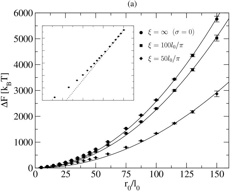
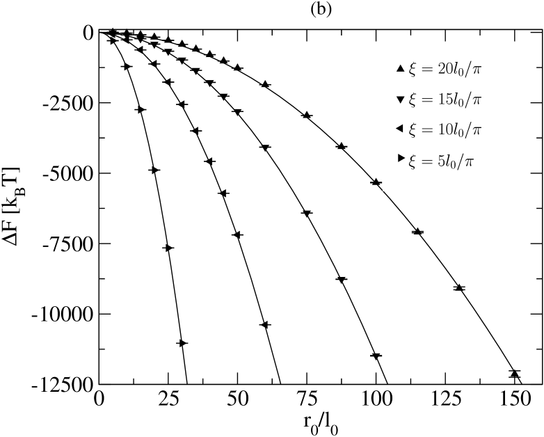
Figure 1: The insertion free energy $\Delta F$ as a function of the inclusion’s radius for $\kappa=10k_{B}T$ and various values of $\sigma_{0}$. The inset to graph (a): a log-log plot of the numerical results for $\sigma_{0}=0$. The slope of the straight dotted line is 2.

In order to obtain an analytical result for the free energy (12), we make the approximation [based on our discussion of the asymptotic behavior of the eigenvalues $\lambda_{1}^{m,n}$, see the text after Eq.(6)] that eigenvalues such that $\lambda_{1}^{m,n}r_{0}<\alpha|m|$ (long wavelength) are not affected by the inclusion, whereas modes with $\lambda_{1}^{m,n}r_{0}>\alpha|m|$ (short wavelength) grow by a factor $L_{p}/(L_{p}-r_{0})$. The numerical constant $\alpha$ is of the order of unity and its value, which may depend on the surface tension $\sigma_{0}$, will be determined later by an exact numerical evaluation of $\Delta F$. We have verified numerically that this asymptotic form is indeed correct. We set $n=0,1,\ldots,\sqrt{N_{0}}$, and, $m=-\sqrt{N_{0}},\ldots,\sqrt{N_{0}}$ so that the total number of modes (degrees of freedom), $2N_{0}$, is proportional to the number of molecules forming the membrane, $N$. Along with these approximations, we evaluate the sum in equation (12) as an integral, giving us the simple result (correct up to quadratic order in $r_{0}$) that $\Delta F=-\pi(\sigma_{0}-\sigma^{*})r_{0}^{2}$, where

$$\sigma^{*}=\frac{k_{B}T}{\pi\alpha\ell_{0}^{2}}\left\{2-\alpha-\left(\frac{\ell_{0}}{\pi\xi}\right)^{2}\ln\left[\left(\frac{\pi\xi}{\ell_{0}}\right)^{2}+1\right]\right\},$$ (13)

$\xi=\sqrt{\kappa/\sigma_{0}}$, and $\ell_{0}=L_{p}/\sqrt{N_{0}}$ is a microscopic length cutoff on the order of the characteristic size of a membrane molecule. We thus obtain the result that the fluctuations renormalize the surface tension. It is interesting to note that this renormalization tends to occur with the opposite sign as the bare surface tension (for $\ell_{0}\lesssim\xi$), thus making it harder to insert an inclusion. Only for very stressed membrane ($\xi\lesssim\ell_{0}$) does $\sigma^{*}$ become negative. This is due to the reduction of the projected area that allows more thermal fluctuations. A more careful analysis of the long wavelength modes shows that these contribute only finite-size effects to the free energy which vanish in the limit of $L_{p}\gg r_{0}$.

We have numerically solved the eigenvalue equation (6) and used the solutions to evaluate the sum in Eq.(12). Numerical values of $\Delta F(r_{0})$ (for $\kappa=10k_{B}T$ and various values of $\sigma_{0}$) are shown in Fig.1 (a)-(b). They have been extracted by extrapolating the numerical results obtained for several values of $750\leq N_{0}\leq 2000$ to the thermodynamic limit $N_{0}\rightarrow\infty$. In the inset to Fig.1 (a), the results for $\sigma_{0}=0$ are replotted on a logarithmic scale, showing that our prediction of a quadratic relation between $\Delta F$ and $r_{0}$ is attained only for large inclusions with $r_{0}\gtrsim 100\ell_{0}$ (the slope of the straight dotted line is 2). This is a typical size for colloidal particles koltover . The value of the constant $\alpha$ appearing in Eq.(13) shows a slight dependence on the surface tension varying from 1.59 for $\sigma_{0}=0$ to 1.72 for $\xi=\sqrt{\kappa/\sigma_{0}}=5l_{0}/\pi$. The solid curves in Fig.1 (a)-(b) depict our analytical expression for $\Delta F$, with $\alpha$ determined by fitting the results for large $r_{0}$ to Eq.(13). From Fig.1 (a) we conclude that, because of thermal fluctuations, there is a free energy penalty to embedding an inclusion in a weakly stretched membrane (small $\sigma_{0}$). For transmembrane proteins with typical radii of $r_{0}\lesssim 5\ell_{0}$, the energy cost is $\Delta F\lesssim 25k_{B}T$, which is comparable to the equilibrium contribution but of opposite sign. This demonstrates the importance of the membrane fluctuations in determining the distribution of transmembrane and free proteins. For larger inclusions, the fluctuation free energy will dominate the equilibrium part. On the other hand, Fig.1 (b) shows that inclusions greatly reduce the free energy of strongly stretched membranes (large $\sigma_{0}$). The primary reason that the free energy is lowered in this regime is the reduction of the projected area. These results should also be relevant for the question of nucleation of a membrane pore which, albeit more complicated, can be studied by similar approach us . They suggest that there exists a (finite!) critical value of the surface tension below which pores cannot open and above which they grow without bounds. Classical nucleation theory, which ignores fluctuations effects, predicts that the critical surface tension is zero nucleationtheory .

In summary, we have computed the free energy of inserting an inclusion into a membrane. We explicitly calculated the contribution of membrane fluctuations. The primary effect of these fluctuations is to reduce the effective value of the surface tension. At low surface tension it provides a positive component to the free energy of an embedded inclusion, thereby impeding the insertion of transmembrane proteins. The sensitivity of the free energy to variations of the surface tension suggests that, by controlling the membrane surface tension appropriately, one may control the thermodynamic stability of embedded proteins and, thus, the equilibrium distribution between proteins inserted in the membrane and in solution.

Acknowledgments: We thank M. Kardar, A.W.C. Lau, and P. Pincus for useful discussions. This work was supported by the NSF under Award No. DMR-0203755. The MRL at UCSB is supported by NSF No. DMR-0080034.

References

- (1) S.A. Safran, Statistical Thermodynamics of Surfaces, Interfaces, and Membranes (Addison-Wesley, New York, 1994).
- (2) R. Lipowsky, E. Sackmann (Editors), Structure and Dynamics of Membranes (Elsevier, Amsterdam, 1995).
- (3) B. Alberts, D. Bray, J. Lewis, M. Raff, K. Roberts, J.D. Watson, Molecular Biology of the Cell (Garland, New York, 1989).
- (4) R. Bruinsma, P. Pincus, Curr. Opin. Solid State Mater. Sci. 1, 401 (1996); M. Kardar, R. Golestanian, Rev. Mod. Phys. 71, 1233 (1999), and references therein.
- (5) S. May, Curr. Opin. Colloid Interface Sci. 5, 244 (2000); M.B. Partenskii, P.C. Jordan, J. Chem. Phys. 117 10768 (2002), and references therein. An exception is the discussion in R.R. Netz, J. Phys. I (France) 7, 833 (1997).
- (6) W. Helfrich, Z. Naturforsch. C 28, 693 (1973).
- (7) A. Ben-Shaul, N. Ben-Tal, B. Honig, Biophys. J. 71, 130 (1996).
- (8) T. Lazaridis, Proteins 52, 176 (2003), and references therein.
- (9) The inner boundary reflects the projection of the cross-sectional area of the inclusion onto the frame reference plane. In the above derivation, we consider a circular boundary with a fixed radius . However, the locus of the inner boundary depend on the tilt angle of the inclusion and varies accordingly. A straightforward calculation us shows that if the tilt angle is small (i.e., when the inner boundary only slightly deviates from circularity) then the boundary of integration in Eq.(1) can be still taken as circular at the expense of introducing an additional boundary term in the Hamiltonian. The new boundary term has no influence on the membrane fluctuations which are governed by the surface Hamiltonian only. Therefore, and for the sake of the simplicity of our derivation, we have dismissed this extra boundary term and its derivation from the discussion.
- (10) P. Sens, S. A. Safran, Europhys. Lett. 43, 95 (1998).
- (11) Corrections to this relation can be neglected when the tilt angle and height of the membrane on the inner boundary are small: , .
- (12) I. Koltover, J. O. Rädler, C. Safinya, Phys. Rev. Lett. 82, 1991 (1999).
- (13) O. Farago, C.D. Santangelo, in preparation.
- (14) J.D. Litster, Phys. Lett. A 53, 193 (1975).