Integrable spin-boson interaction in the Tavis-Cummings model from a generic boundary twist

Luigi Amico(a) and Kazuhiro Hikami(b) $(a)$ Dipartimento di Metodologie Fisiche e Chimiche (DMFCI), UniversitΓ‘ di Catania, viale A. Doria 6, I-95125 Catania, Italy
MATIS &\& Istituto Nazionale per la Fisica della Materia, UnitΓ‘ di Catania, Italy
(b)𝑏(b) Department of Physics, Graduate School of Science, University of Tokyo, Hongo 7-3-1, Bunkyo, Tokyo 113-0033, Japan
Abstract

We construct models describing interaction between a spin $s$ and a single bosonic mode using a quantum inverse scattering procedure. The boundary conditions are generically twisted by generic matrices with both diagonal and off-diagonal entries. The exact solution is obtained by mapping the transfer matrix of the spin-boson system to an auxiliary problem of a spin-$j$ coupled to the spin-$s$ with general twist of the boundary condition. The corresponding auxiliary transfer matrix is diagonalized by a variation of the method of $Q$-matrices of Baxter. The exact solution of our problem is obtained applying certain large-$j$ limit to $su(2)_{j}$, transforming it into the bosonic algebra.

Introduction  Models representing interactions between a single bosonic mode and spin degrees of freedom find application in many different contexts. In atomic physics they describe atoms interacting with electromagnetic fieldΒ [1] and many phenomena like spontaneous emissions in cavityΒ [2] and Rabi oscillationsΒ [3] in two-level atoms are captured by an important representative of the models mentioned above, the Jaynes-Cummings (J-C) modelΒ [4]. Recently the J-C dynamics was intensively studied in the research field of ions in harmonic trapsΒ [5] and then in quantum computationΒ [6]. Finally this kind of models found applications in quasi-2D semiconductors in transverse magnetic fieldΒ [7].
Toy model Hamiltonians representing a single bosonic mode interacting with a spin $s$ are of the following type

H=Hsβˆ’p​h+γ​(S+​a†+Sβˆ’β€‹a)𝐻subscriptπ»π‘ π‘β„Žπ›Ύsuperscript𝑆superscriptπ‘Žβ€ superscriptπ‘†π‘ŽH=H_{s-ph}+\gamma\left(S^{+}a^{\dagger}+S^{-}a\right) (1)

where Hsβˆ’p​h=ω​a†​a+α​Sz+β​(S+​a+Sβˆ’β€‹a†)subscriptπ»π‘ π‘β„Žπœ”superscriptπ‘Žβ€ π‘Žπ›Όsuperscript𝑆𝑧𝛽superscriptπ‘†π‘Žsuperscript𝑆superscriptπ‘Žβ€ H_{s-ph}=\omega a^{\dagger}a+\alpha S^{z}+\beta\left(S^{+}a+S^{-}a^{\dagger}\right); operators a†superscriptπ‘Žβ€ a^{\dagger} and $a$ are bosonic operators that commute with spin operators $S^{v}$, $v=\{z,\pm\}$. The modelΒ (1) with $\gamma=\beta$ was originally proposed for quantum optics purposes to describe a dipole-like interaction in atoms-radiation systems and it is known as the Tavis-Cummings (T-C) model[8]; the model reduces to the J-C one for $s=1/2$. In solid state physics models of type Β (1) can describe certain quantum circuitsΒ [10, 11].

There are two cases in which the model can be solved analytically: i)In the limit sβ†’βˆžβ†’π‘ s\rightarrow\infty there are exact resultsΒ [12]. They were applied to study the entanglement across the quantum phase transition between normal to super-radiant phase[13]. ii) For β€œsingle photon” interactions the model can be simplified employing the Rotating Wave Approximation (RWA) that neglects the so called β€œcounter rotating” terms: S+​a†superscript𝑆superscriptπ‘Žβ€ S^{+}a^{\dagger}, $S^{-}a$. Within the RWA the model (1) can be solved exactly[4, 8, 9]. For generic parameters $\alpha,\beta,\gamma,\omega$, and for finite $s$ the model, as it stands in Eq.Β (1), is non-integrable. Merging the model into the main stream of the Quantum Inverse Scattering (QIS) method[14] constitues often a guide to discover unsuspected exactly solvable models with sufficiently generic interaction. According to this method the Hamiltonian is obtained as output of the procedure that remarkably ensures the integrability of the theory. In the simplest cases the QIS method provide integrable Hamiltonians after periodic boundary condition are imposed. The variety of the integrable models can be considerably enriched by considering more general boundary conditionsΒ [15]. By this is meant that the monodromy matrix is multiplied by non-trivial matrices that ultimately cause the presence of boundary terms in the Hamiltonian. Of interest in the present paper is the case of constant boundary matrix; this realize the, so called, twisted boundary conditions. For the type of models under consideration the QIS method was employed in Ref.[16, 17, 18, 19] where nonlinear generalizations of Hsβˆ’p​hsubscriptπ»π‘ π‘β„ŽH_{s-ph} were studied. These generalizations were obtained by twisting the boundary conditions. The twist matrices were chosen as the same diagonal matrix for both the bosonic and spin degrees of freedom; finally in a certain sense (specified below) they are classical. As a result, although nonlinear, these models contain the standard interaction. Here a more general interaction is obtained applying more general boundary conditions: the twist matrices $K_{B}$ and $K_{S}$ are non-diagonal, different for the boson and the spin, and of β€œquantum” nature (see (5))Β [20]. The Hamiltonian we found is Eq.Β (9). The QIS method pave the way towards the exact solution of the theory through Bethe Ansatz. In the cases where there exist an obvious β€œreference” state a direct (algebraic) Bethe Ansatz approach can be applied. For the model we found here, however, there is no simple vacuum state since (9) does not commute with Sz+a†​asuperscript𝑆𝑧superscriptπ‘Žβ€ π‘ŽS^{z}+a^{\dagger}a. A standard route to attack the exact solutions of such kind of spectral problems is to apply the technique that BaxterΒ [21] invented to obtain the eigenvalues without knowledge of the eigenstates. We obtain the eigenvalues (the calculation of the exact eigenstates will be the object of a future publication) in the following way. We first define an auxiliary problem consisting of two spins with two distinct representations $j$ and $s$; the boundary conditions are generically twisted; the spin $j$ is affected by an β€œimpurity” $\nu$. We diagonalize the auxiliary problem by adapting the Baxter method to it. Then the solution of the spin-bosonic problem is obtained performing certain $j\rightarrow\infty$ limit (see (14)) in the results for the auxiliary spin-spin problem. The eigenvalues are given inΒ (23) and the parameters $\lambda_{k}$ are fixed by (24).

The paper is laid out as follows. In the next section we derive the integrable model. In the section III the exact solution is obtained. The section IV is devoted to our conclusions.

Integrability.  The starting point of the QIS method is to define quantum Lax matrices $L(\lambda)$ and a scattering matrix $R(\lambda)$ satisfying the Yang Baxter (YB) equation: $\displaystyle{R(\lambda-\mu)L(\lambda)\otimes L(\mu)=L(\mu)\otimes L(\lambda)R(\lambda-\mu)\;,}$ where $\lambda$ is the spectral parameter. For the present case, the Lax operators $L$ we consider[17] are

$$L_{S}(\lambda):=\left(\begin{array}[]{cc}\lambda-\eta S^{z}&\eta S^{+}\\ \eta S^{-}&\lambda+\eta S^{z}\end{array}\right)\;,$$ (2)
LB​(Ξ»):=(Ξ»βˆ’Ξ”βˆ’Ξ·βˆ’1βˆ’Ξ·β€‹a†​aa†aβˆ’Ξ·βˆ’1),assignsubscriptπΏπ΅πœ†πœ†Ξ”superscriptπœ‚1πœ‚superscriptπ‘Žβ€ π‘Žsuperscriptπ‘Žβ€ π‘Žsuperscriptπœ‚1L_{B}(\lambda):=\left(\begin{array}[]{cc}\lambda-\Delta-\eta^{-1}-\eta a^{\dagger}a&a^{\dagger}\\ a&-\eta^{-1}\end{array}\right)\;, (3)

each satisfying the YB equation with: $R(\lambda;\eta)=\eta{\rm 1\kern-2.20001ptl}\otimes{\rm 1\kern-2.20001ptl}+\lambda{\rm I\kern-2.5ptP}\;,$ where $\eta\in{\rm\vrule width=0.39993pt,height=6.80275pt,depth=0.0pt\kern-0.39993ptR}$ and ${\rm I\kern-2.5ptP}$ is the permutation: ${\rm I\kern-2.5ptP}A\otimes B{\rm I\kern-2.5ptP}=B\otimes A$. The monodromy matrix is

$$T(\lambda)=K_{B}L_{B}(\lambda)K_{S}L_{S}(\lambda)\;,$$ (4)

where $K_{B}$ and $K_{S}$ are  ${\rm\kern 2.40005pt\vrule width=0.39993pt,height=6.28612pt,depth=-0.3014pt\kern-3.00003ptC}$-number matrices that produce boundary terms (without β€œinternal dynamics”, the matrices $K$ not depending on $\lambda$). Notice that we have two different boundaries each for the spin and for the boson. In Refs.[17, 18] $K_{B}\equiv K_{S}$ is assumed; the T-C model (without counter rotating terms) Hsβˆ’p​hsubscriptπ»π‘ π‘β„ŽH_{s-ph} is obtained for $\eta\rightarrow 0$. The matrix $T(\lambda)$ fulfills the YB relation: $R(\lambda-\mu)T(\lambda)\otimes T(\mu)=T(\mu)\otimes T(\lambda)R(\lambda-\mu)\;,$ due to the fact that $[R,K_{B}\otimes K_{B}]=[R,K_{S}\otimes K_{S}]=0$ holds for any numeric matrix because of the $sl(2)$ symmetry of the $R$-matrix. The transfer matrix is defined as $t(\lambda):=tr_{(0)}T(\lambda)\;$ where $tr_{(0)}$ means trace in the auxiliary space. $t(\lambda)$ is a generating functional of integrals of motion since: $[t(\lambda),t(\mu)]=0$. For the present case the transfer matrix can be chosen as a polynomial in $\eta$: $t(\lambda)=\sum_{l=-g}^{h}\eta^{l}t_{l}(\lambda)$; then the coefficients of $[t(\lambda),t(\mu)]=\sum_{l=-2g}^{2h}\eta^{l}C_{l}(\lambda,\mu)$ vanish at any $\eta$-power. The following assumption is crucial for our purposes: The entries of the matrices $K$ depend on $\eta$

$$K_{X\,ij}=K_{X\,ij}^{(0)}+K_{X\,ij}^{(1)}\eta+\dots\;,\qquad X=\{B,S\}.$$ (5)

The parameter $\eta$ is usually called β€œquantum parameter” since it controls the limit how to recover the classical scattering matrix $r(\lambda)$ from the matrix $R(\lambda)$. In this sense our matrices $K$ in (5) describe β€œquantum systems” which we couple to the the boson and to the spin at the boundary (twist matrices that are independent on $\eta$ might be considered as classical boundaries). In brief, the main idea of our procedure is to play with the boundaries $K$ in such a way that $C_{l}(\lambda,\mu)=0\,\Leftrightarrow\,[t_{l}(\lambda),t_{l}(\mu)]=0$ for certain $l$. In order to obtain the model we are interested in, the degree and the coefficients of the polynomials are fixed such that: i) $t_{m}(\lambda)$ describes an integrable model, then $t_{l}(\lambda)$ must be  ${\rm\kern 2.40005pt\vrule width=0.39993pt,height=6.28612pt,depth=-0.3014pt\kern-3.00003ptC}$-numbers for all $l<m$; ii) the model results containing the counter-rotating terms; iii) the obtained operator is Hermitian. All these conditions translate in a system of equations for the entries of the matrices $K$; we shall see that these parameters will be the coupling constants of the Hamiltonian. It turns out to be sufficient to consider the entries of the $K$ matrices to be linear in $\eta$. Such entries are restricted to

$\displaystyle K_{B\,11}^{(0)}=K_{B\,22}^{(0)}\;,\;K_{S\,11}^{(0)}=K_{S\,22}^{(0)}\;,K_{B\,21}^{(0)}=K_{B\,12}^{(0)}\;,\;{K_{S\,12}^{(0)}}={K_{S\,21}^{(0)}}\;,K_{S\,12}^{(0)}=-\frac{K_{B\,21}^{(0)}K_{S\,22}^{(0)}}{K_{B\,11}^{(0)}}\;,$ (6)
$\displaystyle K_{S\,11}^{(1)}=\frac{K_{B\,22}^{(1)}K_{S\,22}^{(0)}}{K_{B\,11}^{(0)}}+\frac{K_{B\,11}^{(0)}}{K_{B\,12}^{(0)}}(K_{S\,21}^{(1)}-K_{S\,12}^{(1)})-\frac{K_{S\,11}^{(0)}}{K_{B\,12}^{(0)}}(K_{B\,12}^{(1)}-K_{B\,21}^{(1)})+\frac{K_{S\,22}^{(0)}}{K_{B\,11}^{(0)}}K_{B\,11}^{(1)}-K_{S\,22}^{(1)}\;.$ (7)

We take $t_{1}(\lambda)$ as the Hamiltonian

t1​(Ξ»)≐H=W​(Ξ»)​Sz+λ​(U+V)​a†​a+2​[Y+U​V​(Ξ”βˆ’Ξ»)]​Sx+Z​λ​(a+a†)approaches-limitsubscript𝑑1πœ†π»π‘Šπœ†superscriptπ‘†π‘§πœ†π‘ˆπ‘‰superscriptπ‘Žβ€ π‘Ž2delimited-[]π‘Œπ‘ˆπ‘‰Ξ”πœ†superscript𝑆π‘₯π‘πœ†π‘Žsuperscriptπ‘Žβ€ \displaystyle t_{1}(\lambda)\doteq H=W(\lambda)S^{z}+\lambda(U+V)a^{\dagger}a+2\left[Y+\sqrt{UV}(\Delta-\lambda)\right]S^{x}+Z\lambda(a+a^{\dagger}) (8)
βˆ’U​(a​S++a†​Sβˆ’)+V​(a†​S++a​Sβˆ’)βˆ’2​U​V​(a+a†)​Sz,π‘ˆπ‘Žsuperscript𝑆superscriptπ‘Žβ€ superscript𝑆𝑉superscriptπ‘Žβ€ superscriptπ‘†π‘Žsuperscript𝑆2π‘ˆπ‘‰π‘Žsuperscriptπ‘Žβ€ superscript𝑆𝑧\displaystyle-U(aS^{+}+a^{\dagger}S^{-})+V(a^{\dagger}S^{+}+aS^{-})-2\sqrt{UV}(a+a^{\dagger})S^{z}\;, (9)

where the couplings are

$\displaystyle W(\lambda)=-\frac{(U+V)Z}{\sqrt{UV}}+(V-U)(\Delta-\lambda-\frac{Y}{\sqrt{UV}})\;,$ (13)
$\displaystyle U=-K_{B\,22}^{(0)}K_{S\,22}^{(0)}\;,\;V=-{K_{B\,22}^{(0)}(K_{S\,21}^{(0)})^{2}}/{K_{S\,22}^{(0)}}$
$\displaystyle Y=K_{B\,21}^{(0)}\left({K_{B\,11}^{(1)}K_{S\,21}^{(0)}}/{K_{B\,22}^{(0)}}-K_{S\,21}^{(1)}\right)-K_{B\,12}^{(0)}K_{S\,22}^{(1)}-K_{B\,22}^{(0)}K_{S\,12}^{(1)}\;,$
$\displaystyle Z=Y+K_{B\,22}^{(0)}\left(K_{S\,12}^{(1)}+K_{S\,21}^{(1)}\right)+2K_{B\,22}^{(1)}K_{S\,21}^{(0)}\;.$

The coupling constants obeyΒ (13)Β for the model to be integrable; parameters $\Delta$, $\lambda$, $X$, $Z$ can be set freely; the quantity $UV$ must be positive. Nevertheless the rotating and counter-rotating terms can be adjusted to have the same sign by acting on the operators: $S^{-}\rightarrow S^{-}e^{i\frac{\pi}{2}}$ and $a\rightarrow ae^{i\frac{\pi}{2}}$; the third, fourth and last terms in Eq.Β (9) are transformed accordingly. We observe that the simultaneous presence of rotating and counter-rotating terms preserves the integrability only if a further term (a+a†)​Szπ‘Žsuperscriptπ‘Žβ€ superscript𝑆𝑧(a+a^{\dagger})S^{z} appears in the model (the term a+aβ€ π‘Žsuperscriptπ‘Žβ€ a+a^{\dagger} can be transformed out by a translation: $a\rightarrow a+\xi$ with $\xi=-Z/(U+V)$; the coefficients of $S^{x}$ and $S^{z}$ are shifted by $\xi(U-V)$ and $-2\xi\sqrt{UV}$ respectively). Restricting the boundary conditions: $K_{B}=K_{S}$ (non-diagonal) induces the further constraint $U=V$. In this case our model reduces to the Rashba Hamiltonian in a constant magnetic fieldΒ [22] (the bosonic number labeling the Landau levels; see also Ref.[23]).

The constants of motion of (9) are $t_{1}(0)$ and $\partial_{\lambda}t_{1}(\lambda)$ (only two of $H$, $t_{1}(0)$, $\partial_{\lambda}t_{1}(\lambda)$ are independent).Β βˆ‚Ξ»t1​(Ξ»)subscriptπœ†subscript𝑑1πœ†\partial_{\lambda}t_{1}(\lambda) can be easily diagonalized : ${\cal U}\partial_{\lambda}t_{1}(\lambda){\cal U}^{-1}|\phi\rangle=((U+V)(n+m)-M_{-})|\phi\rangle$. In the $|\phi\rangle$ basis the Hilbert space of the Hamiltonian blocks into invariant subspaces labelled by the bosonic number $n\geq 0$ and with $S^{z}|\phi\rangle=m|\phi\rangle$; $M_{-}\doteq Z^{2}/(U+V)$. This will be used to classify the excitations in the Bethe equations (24).

Exact eigenvalues. To diagonalize the model (9) we define an auxiliary inhomogeneous spin problem. We use the property that a spin $j$-$su(2)$ can be contracted to the Weyl-Heisenberg algebraΒ [24] through the singular limit $\varepsilon\rightarrow\infty$ of a Dyson-Maleev transformation

{βˆ’Ξ·β€‹Jβˆ’,1η​Ρ2​J+,Jz}↦{a†,a,βˆ’a†​aβˆ’Ξ΅22};maps-toπœ‚superscript𝐽1πœ‚superscriptπœ€2superscript𝐽superscript𝐽𝑧superscriptπ‘Žβ€ π‘Žsuperscriptπ‘Žβ€ π‘Žsuperscriptπœ€22\left\{-\eta J^{-},\;\frac{1}{\eta\varepsilon^{2}}J^{+},\;J^{z}\right\}\mapsto\left\{a^{\dagger},\;a,\;-a^{\dagger}a-\frac{\varepsilon^{2}}{2}\right\}\;; (14)

such a limit corresponds to $j=-\varepsilon^{2}/2\rightarrow\infty$. The bosonic Lax matrix is thus expressed as limit of a spin-$j$ Lax matrix:

$${L}_{B}(\lambda)=\lim_{\varepsilon\rightarrow\infty}(-\frac{1}{\eta\varepsilon})K(\varepsilon)\sigma_{y}\sigma_{z}{L}_{J}(\lambda-\nu)\sigma_{y}\;,$$ (15)

where $K(\varepsilon)=diag\left\{\eta\varepsilon,(\eta\varepsilon)^{-1}\right\}$ and

$${L}_{J}(\lambda-\nu)=\left(\begin{array}[]{cc}\lambda-\nu-\eta J^{z}&\eta J^{+}\\ \eta J^{-}&\lambda-\nu+\eta J^{z}\end{array}\right)\;,$$ (16)

the β€œinhomogeneity” parameter being set to

$$\nu=-\eta\varepsilon^{2}/2+\eta^{-1}+\Delta\;.$$ (17)

Thus the monodromy matrix EqΒ (4) can be written as $T(\lambda)=\lim_{\epsilon\rightarrow\infty}T_{a}(\lambda)$ where $T_{a}$ is an auxiliary monodromy matrix defined as

$$T_{a}\doteq K_{J}L_{J}(\lambda-\nu)\sigma_{y}K_{S}L_{S}(\lambda)\;,$$ (18)

with $K_{J}\doteq-1/(\eta\varepsilon)K_{B}K(\epsilon)\sigma_{y}\sigma_{z}$. $t_{a}=tr_{0}\{T_{a}\}$ can be diagonalized adapting the Baxter methodΒ [21] for off-diagonal twisted spin-$s$ chainΒ [25]. In the present case the β€œchain” consists of only two sites; the twist matrices are distinct and containing both diagonal and off-diagonal entries. The details of the calculations will be reported elsewhere. The Baxter equation reads

ta​(Ξ»)​Q​(Ξ»)=R(βˆ“)​(Ξ»βˆ’s​η)​(Ξ»βˆ’Ξ½βˆ’j​η)​Q​(Ξ»+Ξ·)+R(Β±)​(Ξ»+s​η)​(Ξ»βˆ’Ξ½+j​η)​Q​(Ξ»βˆ’Ξ·),subscriptπ‘‘π‘Žπœ†π‘„πœ†superscript𝑅minus-or-plusπœ†π‘ πœ‚πœ†πœˆπ‘—πœ‚π‘„πœ†πœ‚superscript𝑅plus-or-minusπœ†π‘ πœ‚πœ†πœˆπ‘—πœ‚π‘„πœ†πœ‚\displaystyle t_{a}(\lambda)Q(\lambda)=R^{(\mp)}\;(\lambda-s\eta)(\lambda-\nu-j\eta)Q(\lambda+\eta)+{R^{(\pm)}}\,(\lambda+s\eta)(\lambda-\nu+j\eta)Q(\lambda-\eta)\;, (19)

where $R^{(\pm)}\doteq\frac{1}{2}\left[tr(K_{J}\sigma_{y}K_{S})\pm\sqrt{(tr(K_{J}\sigma_{y}K_{S}))^{2}+4\det(K_{J}K_{S})}\right]$. The quantities $Q(\lambda)$ are $(2s+2j+2)\times(2s+2j+2)$ matrices and constructed in the standard way[21, 25]; they fulfill $[Q(\lambda),Q(\mu)]=[Q(\lambda),t_{a}(\lambda)]=0$. EqΒ (19) fixes the eigenvalue $\tau_{a}(\lambda)^{(\pm)}$ of the transfer matrix

Ο„a​(Ξ»)(Β±)=R(βˆ“)​(Ξ»βˆ’s​η)​(Ξ»βˆ’Ξ½βˆ’j​η)subscriptπœπ‘Žsuperscriptπœ†plus-or-minussuperscript𝑅minus-or-plusπœ†π‘ πœ‚πœ†πœˆπ‘—πœ‚\displaystyle\tau_{a}(\lambda)^{(\pm)}=R^{(\mp)}\;(\lambda-s\eta)(\lambda-\nu-j\eta) $\displaystyle\prod_{i=1}^{2s+2j}\frac{\lambda-\lambda_{i}+\eta}{\lambda-\lambda_{i}}$ (21)
+R(Β±)​(Ξ»+s​η)​(Ξ»βˆ’Ξ½+j​η)β€‹βˆi=12​s+2​jΞ»βˆ’Ξ»iβˆ’Ξ·Ξ»βˆ’Ξ»i,superscript𝑅plus-or-minusπœ†π‘ πœ‚πœ†πœˆπ‘—πœ‚superscriptsubscriptproduct𝑖12𝑠2π‘—πœ†subscriptπœ†π‘–πœ‚πœ†subscriptπœ†π‘–\displaystyle+R^{(\pm)}\,(\lambda+s\eta)(\lambda-\nu+j\eta)\prod_{i=1}^{2s+2j}\frac{\lambda-\lambda_{i}-\eta}{\lambda-\lambda_{i}}\;,

where the variables $\lambda_{j}$ are solutions of the equations

R(βˆ“)R(Β±)​(Ξ»kβˆ’s​η)​(Ξ»kβˆ’Ξ½βˆ’j​η)(Ξ»k+s​η)​(Ξ»kβˆ’Ξ½+j​η)=∏i=1iβ‰ k2​s+2​jΞ»kβˆ’Ξ»iβˆ’Ξ·Ξ»kβˆ’Ξ»i+Ξ·,k=1,…,2​(s+j).formulae-sequencesuperscript𝑅minus-or-plussuperscript𝑅plus-or-minussubscriptπœ†π‘˜π‘ πœ‚subscriptπœ†π‘˜πœˆπ‘—πœ‚subscriptπœ†π‘˜π‘ πœ‚subscriptπœ†π‘˜πœˆπ‘—πœ‚superscriptsubscriptproductFRACOP𝑖1π‘–π‘˜2𝑠2𝑗subscriptπœ†π‘˜subscriptπœ†π‘–πœ‚subscriptπœ†π‘˜subscriptπœ†π‘–πœ‚π‘˜1…2𝑠𝑗\frac{R^{(\mp)}}{R^{(\pm)}}\frac{(\lambda_{k}-s\eta)(\lambda_{k}-\nu-j\eta)}{(\lambda_{k}+s\eta)(\lambda_{k}-\nu+j\eta)}=\prod_{i=1\atop i\neq k}^{2s+2j}\frac{\lambda_{k}-\lambda_{i}-\eta}{\lambda_{k}-\lambda_{i}+\eta}\;,\qquad\qquad\;k=1,\dots,2(s+j)\;. (22)

To obtain the solution of the bosonic problem we perform the algebraic contraction at the level of Eqs.Β (22). This can be done expanding ${R^{(\pm)}=\sum_{m}R^{(\pm)}_{2m}/(\varepsilon\eta)^{2m}}$ and taking into account of Eq.Β (17); a generalizations of the Bethe equations found inΒ [17] are obtained. By a further expansion $R^{(\pm)}_{2m}=\sum_{n=0}^{2}R^{(\pm)}_{2m,n}\eta^{n}$ in the latter equations, the eigenvalues ${\cal E}$ of the model (9) can be obtained as their linear terms in $\eta$:

β„°=β„°0​(Ξ»)+βˆ‘j=12​s+n1Ξ»βˆ’Ξ»j​[βˆ’Ξ»β€‹x0βˆ’β€‹βˆ‘lβ‰ j2​s+n1Ξ»jβˆ’Ξ»lβˆ’Ξ»β€‹(Ξ»βˆ’Ξ”)​y0βˆ’βˆ’Ξ»β€‹x1++s​x0βˆ’],β„°subscriptβ„°0πœ†superscriptsubscript𝑗12𝑠𝑛1πœ†subscriptπœ†π‘—delimited-[]πœ†subscriptsuperscriptπ‘₯0superscriptsubscript𝑙𝑗2𝑠𝑛1subscriptπœ†π‘—subscriptπœ†π‘™πœ†πœ†Ξ”subscriptsuperscript𝑦0πœ†subscriptsuperscriptπ‘₯1𝑠subscriptsuperscriptπ‘₯0\displaystyle{\cal E}={\cal E}_{0}(\lambda)+\sum_{j=1}^{2s+n}\frac{1}{\lambda-\lambda_{j}}\left[-\lambda x^{-}_{0}\sum_{l\neq j}^{2s+n}\frac{1}{\lambda_{j}-\lambda_{l}}-\lambda(\lambda-\Delta)y^{-}_{0}-\lambda x^{+}_{1}+sx^{-}_{0}\right]\;, (23)

where ${\cal E}_{0}(\lambda)=(\lambda-\Delta)(\lambda y^{+}_{1}+sy^{-}_{0})-\lambda x^{-}_{2}+sx^{+}_{1}$; with $x^{\alpha}_{n}=R^{(\mp)}_{0,n}-\alpha R^{(\pm)}_{0,n}-R^{(\mp)}_{2,n}$ and $y^{\alpha}_{n}=R^{(\pm)}_{0,n}+\alpha R^{(\mp)}_{0,n}$ $\alpha=\{+,-\}$. The quantities $\lambda_{k}$ are fixed by

s​x0βˆ’Ξ»kβˆ’(Ξ»kβˆ’Ξ”)​y0βˆ’=x0βˆ’β€‹βˆ‘lβ‰ k2​s+n1Ξ»kβˆ’Ξ»l+x1+,𝑠subscriptsuperscriptπ‘₯0subscriptπœ†π‘˜subscriptπœ†π‘˜Ξ”subscriptsuperscript𝑦0subscriptsuperscriptπ‘₯0superscriptsubscriptπ‘™π‘˜2𝑠𝑛1subscriptπœ†π‘˜subscriptπœ†π‘™subscriptsuperscriptπ‘₯1\frac{sx^{-}_{0}}{\lambda_{k}}-\left(\lambda_{k}-\Delta\right)y^{-}_{0}=x^{-}_{0}\sum_{l\neq k}^{2s+n}\frac{1}{\lambda_{k}-\lambda_{l}}+x^{+}_{1}\,, (24)

where $k=1,\dots,2s+n$; the quantum number $n$ labels the excitations as discussed before. For generic $2s+n$ the equations above can be solved numerically. Alternatively the quantities $\lambda_{k}$ can be obtained as roots of the polynomial P​(Ξ»)=∏s=12​s+n(Ξ»βˆ’Ξ»s)π‘ƒπœ†superscriptsubscriptproduct𝑠12π‘ π‘›πœ†subscriptπœ†π‘ P(\lambda)=\prod_{s=1}^{2s+n}(\lambda-\lambda_{s}) satisfying

λ​P′′​(Ξ»)+2x0βˆ’β€‹[y0βˆ’β€‹Ξ»2+(y0βˆ’β€‹Ξ”+x1+)β€‹Ξ»βˆ’s​x0βˆ’]​P′​(Ξ»)βˆ’[ΞΆβˆ’(2​s+n)​λ]​P​(Ξ»)=0πœ†superscriptπ‘ƒβ€²β€²πœ†2subscriptsuperscriptπ‘₯0delimited-[]subscriptsuperscript𝑦0superscriptπœ†2subscriptsuperscript𝑦0Ξ”subscriptsuperscriptπ‘₯1πœ†π‘ subscriptsuperscriptπ‘₯0superscriptπ‘ƒβ€²πœ†delimited-[]𝜁2π‘ π‘›πœ†π‘ƒπœ†0\lambda P^{\prime\prime}(\lambda)+\frac{2}{x^{-}_{0}}\left[y^{-}_{0}\lambda^{2}+(y^{-}_{0}\Delta+x^{+}_{1})\lambda-sx^{-}_{0}\right]P^{\prime}(\lambda)-\left[\zeta-(2s+n)\lambda\right]P(\lambda)=0 (25)

where $\zeta$ is fixed by imposing that $\lambda=0$ is a simple root of $\lambda P(\lambda)$: ΞΆ=s​x0βˆ’β€‹P′​(0)P​0πœπ‘ subscriptsuperscriptπ‘₯0superscript𝑃′0𝑃0\zeta=sx^{-}_{0}\frac{P^{\prime}(0)}{P{0}}Β [17].

Conclusions. By the Quantum Inverse scattering method we have constructed integrable T-C models with twisted boundary conditions. The twist matrices are generic in the sense that they contain both diagonal and non-diagonal entries. They are responsible for the presence of rotating and counter-rotating terms in the Hamiltonian. The spectrum is computed through the Baxter method. As far as we know this method is applied to spin-boson systems for the first time; the subtleties related to the bosonic limit, recovered for infinite spin length are dug out. Integrability and exact solution can be obtained provided that a further term ∝(a+a†)​Szproportional-toabsentπ‘Žsuperscriptπ‘Žβ€ superscript𝑆𝑧\propto(a+a^{\dagger})S^{z} is considered. Interestingly enough we found a global rotation of the spin/bosonic degrees of freedom such that the rotating terms (alternatively, the counter-rotating terms) are compensated out[29]. We conjecture that β€œtrue” counter-rotating terms in the Tavis-Cummings model could be inserted considering dynamical boundaries: KX=KX​(Ξ»)subscript𝐾𝑋subscriptπΎπ‘‹πœ†K_{X}=K_{X}(\lambda); alternatively one should consider X​Y​Zπ‘‹π‘Œπ‘XYZ symmetry of the scattering matrix. These terms serve to a reliable description of certain systems in quantum optics[26, 27] or to model the spin-orbit interaction in heterostructures where the simultaneous Rashba and Dresselhaus terms are important[30]. Our paper could pave the way to costruct integrable Hamiltonians for such physical situations. 
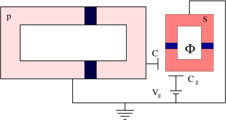
As immediate application, we notice that the Hamiltonian (9) describes the quantum circuit of Fig.(1). Two coupled dc-Superconducting Quantum Interference Devices (SQUIDs) are coupled inductively. The primary device p𝑝p is intended built with large Josephson junctions to be described by a classical SQUID Hamiltonian[31] (whose degrees of freedom are, then, bosonic) flowed by the current Ipsubscript𝐼𝑝I_{p} (this circuit plays the role of the L​C𝐿𝐢LC resonant circuit of Ref.Β [11]); the secondary SQUID s𝑠s, with small junctions, is accommodated inside the primary and pierced by the magnetic flux: Ξ¦=Ο•e​x​t+Lp​IpΞ¦subscriptitalic-ϕ𝑒π‘₯𝑑subscript𝐿𝑝subscript𝐼𝑝\Phi=\phi_{ext}+L_{p}I_{p} (Lpsubscript𝐿𝑝L_{p} is the inductance of the circuit). Thus the secondary is a quantum SQUID controlled by the classical one.

Refer to caption
FIG. 1.: The quantum circuit described by the Hamiltonian (26). The primary device $p$ is a resonant circuit controlling the flux-qubit $s$ by the inductive coupling caused by $\Phi=\phi_{ext}+L_{p}I_{p}$.

The effective Josephson coupling of the quantum SQUID depends on the flux $E_{J}^{s}(\Phi)\simeq E_{J}^{s}(\phi_{ext})+\tilde{L}_{p}I_{p}$ . This kind of setups are intensively studied as controllable flux-qubits[32, 33] to data-bus transferring in many protocols of quantum computation[11]. The circuit Hamiltonian is

β„‹c​i​r​c​u​i​t=Ο‰p​a†​aβˆ’2​EJs​(Ο•e​x​t)​Sxβˆ’2​L~p​(a+a†)​Sxβˆ’i​M​(aβˆ’a†)​Sy+2​VC​(a+a†)​Szsubscriptβ„‹π‘π‘–π‘Ÿπ‘π‘’π‘–π‘‘subscriptπœ”π‘superscriptπ‘Žβ€ π‘Ž2subscriptsuperscript𝐸𝑠𝐽subscriptitalic-ϕ𝑒π‘₯𝑑superscript𝑆π‘₯2subscript~πΏπ‘π‘Žsuperscriptπ‘Žβ€ superscript𝑆π‘₯π‘–π‘€π‘Žsuperscriptπ‘Žβ€ superscript𝑆𝑦2subscriptπ‘‰πΆπ‘Žsuperscriptπ‘Žβ€ superscript𝑆𝑧{\cal H}_{circuit}=\omega_{p}a^{\dagger}a-2E^{s}_{J}(\phi_{ext})S^{x}-2\tilde{L}_{p}(a+a^{\dagger})S^{x}-iM(a-a^{\dagger})S^{y}+2V_{C}(a+a^{\dagger})S^{z} (26)

where $\omega_{p}$ is the β€œfrequency” of the primary SQUID (or the natural frequency of the resonant circuit[11]), $V_{C}$ is due to the capacitive coupling between the SQUID’s; $E_{J}^{\alpha},\;E_{C}^{\alpha}\;,\alpha=\{p,s\}$ are related respectively to the Josephson and the charging energies of the junctions and $M$ is the mutual inductance; the gate voltage $V_{g}$ is tuned to the charge degeneracy point[31]. For generic circuit-parameters the dynamics of the qubit is intricated by the presence of the counter-rotating terms, making the device not reliable in the communication protocols. Our calculation suggests how the circuit parameters can be tuned to reproduce our model (9); for it the dynamics is not altered by the presence of the counter-rotating terms. Using this trick the qubit dynamics can be effectively β€œprotected” at any frequency $\omega_{p}$. The relation between the circuit-parameters and coefficients in the Hamiltonian (9) is: $\{\omega_{p},E^{s}_{J},2\tilde{L}_{p},M,V_{C}\}\rightarrow\{\lambda(U+V),2Y,U+V,U-V,-2\sqrt{UV}\}$ ($Z=0$ is set for simplicity), implying that $V_{C}$ should be tuned to $V_{C}=\sqrt{M^{2}-4\tilde{L_{p}}^{2}}/2$ to make un-effective the counter-rotating terms.

Acknowledgements.
Discussions with G. Falci and A. Osterloh are acknowledged. We are grateful to D. Averin, P. Kulish, E. Paladino, R. Fazio and R. Richardson for helpful comments. While completing this paper, equations similar toΒ (19)-(22) appeared in [28].

REFERENCES

  • [1] C. Cohen-Tannoudji, J. Dupont-Roc, and G. Grynberg, Atom-photon interactions (Wiley, New York 1992).
  • [2] D. Kleppner, Phys. Rev. Lett. 47, 233 (1981).
  • [3] G. Rempe, F. Schmidt-Kaler, and H. Walther, Phys. Rev. Lett. 64, 2783 (1990).
  • [4] E.T. Jaynes and F.W. Cummings, Proc. IEEE 51, 89 (1963).
  • [5] J.I. Cirac, et al., Phys. Rev. A 46, 2668 (1992).
  • [6] R. J. Hughes, et al., Fortsch. Phys. 46, 329 (1998).
  • [7] S. Datta and B. Das, Appl. Phys. Lett. 56, 665 (1990); L. W. Molenkamp, G. Schmidt, and G. E. W. Bauer, Phys. Rev. B 64, 121202 (2001).
  • [8] M. Tavis and F.W. Cummings, Phys. Rev. 170, 379 (1969); ibid. 188, 692 )(1969).
  • [9] K. Hepp and E. Lieb, Ann. Phys. 76, 360 (1973).
  • [10] T. Brandes, N. Lambert, Phys. Rev. B 67, 125323 (2003).
  • [11] M. Paternostro, et al., Phys. Rev. B 69, 214502 (2004); F. Plastina and G. Falci, Phys. Rev. B 67, 224514 (2003).
  • [12] C. Emary and T. Brandes, Phys. Rev. E 67, 066203, (2003).
  • [13] N. Lambert, C. Emary, and T. Brandes, Phys. Rev. Lett. 92, 073602 (2004).
  • [14] V.E. Korepin, N.M. Bogoliubov, and A.G. Izergin, Quantum Inverse Scattering Method and Correlation Functions, (Cambridge Univ. Press, Cambridge 1993).
  • [15] E. Sklyanin, J. Phys. A 21 , 2375 (1988).
  • [16] B. Jurco, J. Math. Phys. 30, 1739 (1989).
  • [17] N.M. Bogoliubov, R.K. Bullough, and J. Timonen, J. Phys. A 29, 6305 (1996).
  • [18] A. Rybin, et al , J. Phys. A 31, 4705 (1998).
  • [19] A. Kundu, Phys. Rev. Lett. 82, 3936 (1999); ibid. quant-ph/0307102.
  • [20] A. Di Lorenzo, et al. Nucl. Phys. B. 644, 409 (2002).
  • [21] R.J. Baxter, Exactly solved models in statistical mechanics, (Academic Press, London 1982).
  • [22] E.I. Rashba, Sov. Phys. Solid State 2, 1109 (1960).
  • [23] C. Emary and T. Brandes, Phys. Rev. A 69, 053804 (2004).
  • [24] R. Gilmore, Lie groups, Lie algebras, and some of their applications (Wiley, New York, 1974).
  • [25] C.M. Yung and M.T. Batchelor, Nucl.Phys. B446, 461 (1995).
  • [26] D.M. Meekhof et al, Phys. Rev. Lett. 76, 1796 (1996).
  • [27] C. D’Helon and G.J. Milburn, quant-ph/9705014.
  • [28] G.A.P. Ribeiro, M.J. Martins, and W. Galleas, Nucl. Phys. B, 675, 567 (2003).
  • [29] Ultimately, this results to preserve the integrability of the Hamiltonian. It can be proved that off-diagonal are equivalent to diagonal twists for $SU(N)$ models, ancestors of the spin-boson models (see also W. Galleas, M.J. Martins, nlin.SI/0407027).
  • [30] J. Schliemann, J. C. Egues, and D. Loss, Phys. Rev. B 67, 085302 (2003).
  • [31] M. Tinkham, Introduction to superconductivity, (Mc Graw-Hill, New York 1996).
  • [32] I. Chiorescu et. al., Nature 431, 159 (2004); P. Orlando et al., Science 285, 1036 (1999).
  • [33] K.V.R.M. Murali, et al., cond-mat/0311471.