Liquid Crystals in Electric Field

Abstract

We present a general theory of electric field effects in liquid crystals where the dielectric tensor depends on the orientation order. As applications, we examine (i) the director fluctuations in nematic states in electric field for arbitrary strength of the dielectric anisotropy and (ii) deformation of the nematic order around a charged particle. Some predictions are made for these effects.

1 Introduction

Phase transitions occur in various systems in electric field. To treat such problems we need to construct a Ginzburg-Landau free energy including electrostatic interactions and electric field effects under each given boundary condition[1]. The gross variables include the order parameter $\psi$, the polarization $p$, and the charge density $\rho$. (Note $\psi={\mbox{\boldmath$p$}}$ in ferroelectric systems.) In this letter we present such a theory for liquid crystals in nematic states[2], since there seems to be no systematic theory of electric field effects for anisotropic fluids. We also examine the deformation of the director around a charged particle, since the nematic order around a neutral colloid particle or emulsion droplet has been extensively studied[3, 4]. We shall see that the charge-induced orientation is intensified with decreasing the particle radius $R$ and/or increasing the charge number $Z$, while the surface anchoring of a neutral particle can be achieved for large radius because the penalty of the Frank free energy needs to be small.

2 Liquid crystals between capacitor plates

In liquid crystals the order parameter $\psi$ represents the orientation tensor near the isotropic-nematic transition or the director $n$ in nematic states. We also use the vector notation $\rho$ to represent the set $\{\rho_{\alpha}\}$ for the ion densities $\rho_{\alpha}$ ($\alpha=1,2,\cdots$). We divide the total free energy functional $F=F_{\rm ch}+F_{\rm st}$ into a chemical part $F_{\rm ch}$ and an electrostatic part $F_{\rm st}$. Here,

$$F_{\rm ch}=F_{0}\{\psi,{\mbox{\boldmath$\rho$}}\}+\int d{\mbox{\boldmath$r$}}\frac{1}{2}\sum{{\chi}}^{ij}p_{i}p_{j},$$ (1)

The first contribution $F_{0}$ is assumed to be independent of $p$, but there arises a coupling between $\psi$ and $p$ in the presence of flexoelectricity[2, 5]. The tensor $\chi^{ij}$ is the inverse matrix of the the electric susceptibility tensor $\chi_{ij}$. We shall see that the local dielectric tensor ${\varepsilon}_{ij}$ is related to $\chi_{ij}$ as

$$\varepsilon_{ij}=\delta_{ij}+4\pi\chi_{ij}.$$ (2)

As is well-known, $\varepsilon_{ij}$ depends on the orientation order. In particular, in nematic states the following form has been assumed in agreement with experiments:[2]

$$\varepsilon_{ij}=\varepsilon_{0}\delta_{ij}+\varepsilon_{1}n_{i}n_{j}.$$ (3)

The coefficients $\varepsilon_{0}$ and $\varepsilon_{1}$ satisfy $\varepsilon_{0}>1$ and $\varepsilon_{0}+\varepsilon_{1}>1$ because $\chi_{ij}$ should be a positive-definite matrix from the thermodynamic stability.

Next we consider the electrostatic part $F_{\rm st}$. A typical experimental geometry is shown in Fig.1a, where we insert our system between two parallel metallic plates with area $S$ and separation distance $L$. We assume $S^{1/2}\gg L$ and neglect the effects of edge fields. The $z$ axis is taken perpendicularly to the plates. Let the average surface charge density of the upper plate be $\sigma_{\rm ex}$ and that of the lower plate be $-\sigma_{\rm ex}$. The total charge on the upper plate is ${Q}=S\sigma_{\rm ex}$. The electric potential $\phi$ satisfies $\phi=0$ at the bottom $z=0$ and $\phi=\Phi$ at the top $z=L$, where $\Phi$ is the potential difference between the two capacitor plates. The electric induction $\mbox{\boldmath$D$}={\mbox{\boldmath$E$}}+4\pi{\mbox{\boldmath$p$}}$ satisfies

$$\nabla\cdot{\mbox{\boldmath$D$}}=-\nabla^{2}\phi+4\pi\nabla\cdot{\mbox{\boldmath$p$}}=4\pi\rho,$$ (4)

where $\rho=\sum_{\alpha}eZ_{\alpha}\rho_{\alpha}$ is the charge density with $Z_{\alpha}e$ being the charge of the ion species $\alpha$. The boundary conditions at $z=0$ and $L$ are $E_{x}=E_{y}=0$ and $D_{z}=-4\pi\sigma_{\rm ex}$ [6]. With these relations $F_{\rm st}$ is of the form,

$$F_{\rm st}=\int d{\mbox{\boldmath$r$}}{\mbox{\boldmath$E$}}^{2}/{8\pi}.$$ (5)

In fact, if infinitesimal deviations $\delta{\mbox{\boldmath$p$}}$, $\delta\rho$, and $\delta{Q}$ are superimposed on $p$, $\rho$, and ${Q}$, the incremental change of $F_{\rm st}$ is given by

$$\delta F_{\rm st}=\int d{\mbox{\boldmath$r$}}[-{\mbox{\boldmath$E$}}\cdot{\delta{\mbox{\boldmath$p$}}}+\phi\delta\rho]+\Phi\delta{Q},$$ (6)

where use is made of $\delta({\mbox{\boldmath$E$}}^{2})=-2{\nabla\phi}\cdot\delta{\mbox{\boldmath$D$}}-8\pi{\mbox{\boldmath$E$}}\cdot\delta{\mbox{\boldmath$p$}}=-2\nabla(\phi\delta{\mbox{\boldmath$D$}})+8\pi(\phi\delta\rho-{\mbox{\boldmath$E$}}\cdot\delta{\mbox{\boldmath$p$}})$. The right hand side of (6) represents the increase of the electrostatic free energy due to the small variations of $p$, $\rho$, and $Q$.

If we minimize $F$ with respect to $p$ for fixed $\psi$, $\rho$, and $Q$, we require $\delta F/\delta{\mbox{\boldmath$p$}}={\mbox{\boldmath$0$}}$. Then (1) and (6) give

$${\mbox{\boldmath$p$}}=\stackrel{{\scriptstyle\leftrightarrow}}{{\mbox{\boldmath$\chi$}}}\cdot{\mbox{\boldmath$E$}},\quad{\mbox{\boldmath$D$}}=\stackrel{{\scriptstyle\leftrightarrow}}{{\mbox{\boldmath$\varepsilon$}}}\cdot{\mbox{\boldmath$E$}},$$ (7)

which indeed yield (2). Then we may rewrite $F$ as $F=F_{0}+F_{\rm e}$ with $F_{\rm e}=\int d{\mbox{\boldmath$r$}}\sum_{ij}\chi^{ij}p_{i}p_{j}/2+F_{\rm st}$, so

$$F_{\rm e}=\frac{1}{8\pi}\int d{\mbox{\boldmath$r$}}{\mbox{\boldmath$E$}}\cdot{{\stackrel{{\scriptstyle\leftrightarrow}}{{\mbox{\boldmath$\varepsilon$}}}}}\cdot{\mbox{\boldmath$E$}}=\frac{1}{8\pi}\int d{\mbox{\boldmath$r$}}{\mbox{\boldmath$E$}}\cdot{\mbox{\boldmath$D$}}.$$ (8)

Under these relations and using $\delta\chi^{ij}=-\sum_{k\ell}\chi^{ik}\chi^{j\ell}\delta\chi_{k\ell}$ we obtain

$$\delta F=\delta F_{0}+\int d{\mbox{\boldmath$r$}}\bigg{[}\phi\delta\rho-\frac{1}{8\pi}{\mbox{\boldmath$E$}}\cdot{\delta{\stackrel{{\scriptstyle\leftrightarrow}}{{\mbox{\boldmath$\varepsilon$}}}}}\cdot{\mbox{\boldmath$E$}}\bigg{]}+\Phi\delta{Q}.$$ (9)

From (4) and (7) the electric potential satisfies

$$-\nabla\cdot\stackrel{{\scriptstyle\leftrightarrow}}{{\mbox{\boldmath$\varepsilon$}}}\cdot\nabla\phi=4\pi\rho.$$ (10)

Thus $\phi$ and ${\mbox{\boldmath$E$}}=-\nabla\phi$ depend on the orientation order via (3) and on $\rho$ under each boundary condition. In the literature[2], however, the electric field $E$ in (9) has been replaced by the average constant field ${\mbox{\boldmath$E$}}_{0}$, where $F=F_{0}-\varepsilon_{1}\int d{\mbox{\boldmath$r$}}({\mbox{\boldmath$E$}}_{0}\cdot{\mbox{\boldmath$n$}})^{2}/8\pi$ +const.+O($\varepsilon_{1}^{2}$). This is the first order approximation with respect to $\varepsilon_{1}$ valid for $|\varepsilon_{1}|\ll\varepsilon_{0}$. If $\varepsilon_{1}+\varepsilon_{0}$ is considerably smaller or larger than $\varepsilon_{0}$, there can be unexplored regimes of strong polarization anisotropy.

So far the capacitor charge ${Q}$ is a control parameter and the potential difference $\Phi$ is a fluctuating quantity dependent on $p$ and $\rho$. We may also control $\Phi$ by using (i) a battery at a fixed potential difference or (ii) connecting another large capacitor in parallel to the capacitor containing our system as in Fig.1b. As will be discussed in the appendix, the appropriate free energy functional is given by the Legendre transformation [6],

$$G=F-\Phi{Q}.$$ (11)

From (9) the incremental change of $G$ is obtained as

$$\delta G=\delta F_{0}+\int d{\mbox{\boldmath$r$}}\bigg{[}\phi\delta\rho-\frac{1}{8\pi}{\mbox{\boldmath$E$}}\cdot{\delta{\stackrel{{\scriptstyle\leftrightarrow}}{{\mbox{\boldmath$\varepsilon$}}}}}\cdot{\mbox{\boldmath$E$}}\bigg{]}-{Q}\delta\Phi.$$ (12)

3 Director fluctuations in nematic states

As a first application of our theory, we apply an electric field $E_{0}$ to a nematic liquid crystal considerably below the transition without charges ($\rho=0$), where the orientation order is represented by the director vector $n$. Here we do not perform the expansion with respect to $\varepsilon_{1}$. For simplicity, we assume that $n$ is along the $z$ axis on the average under the homeotropic boundary condition and $\varepsilon_{1}>0$. If $\varepsilon_{1}<0$, the orientation along the $z$ axis becomes unstable with increasing $E_{0}$ above a critical value $(\propto L^{-1})$[2]. Then $n$ is written as ${\mbox{\boldmath$e$}}_{z}+\delta{\mbox{\boldmath$n$}}$ with $\delta n_{z}=-[(\delta n_{x})^{2}+(\delta n_{y})^{2}]/2$, where ${\mbox{\boldmath$e$}}_{z}$ is the unit vector along the $z$ axis and $\delta{\mbox{\boldmath$n$}}$ is the deviation nearly perpendicular to the $z$ axis. By solving (10) under (3), we may expand the electrostatic free energy $F_{\rm e}=F-F_{0}$ in powers of $\delta{\mbox{\boldmath$n$}}$. The fluctuation contributions on the bilinear order are written as

$$\Delta F_{\rm e}=\frac{\varepsilon_{1}}{8\pi}E_{0}^{2}\int_{\mbox{\boldmath$q$}}\bigg{[}|\delta{\mbox{\boldmath$n$}}({\mbox{\boldmath$q$}})|^{2}+\frac{\varepsilon_{1}}{\varepsilon_{0}+\varepsilon_{1}\hat{q}_{z}^{2}}|\hat{{\mbox{\boldmath$q$}}}\cdot\delta{\mbox{\boldmath$n$}}({\mbox{\boldmath$q$}})|^{2}\bigg{]},$$ (13)

where $\hat{\mbox{\boldmath$q$}}=q^{-1}{\mbox{\boldmath$q$}}$ represents the direction of $q$ and ${\mbox{\boldmath$n$}}({\mbox{\boldmath$q$}})$ is the Fourier transform of $\delta{\mbox{\boldmath$n$}}$. The wave number $|{\mbox{\boldmath$q$}}|$ is assumed to be much larger than the inverse system width $L^{-1}$. The large scale fluctuations are omitted in (13).

Expressing $F_{0}$ in terms of the Frank constants $K_{1}$, $K_{2}$, and $K_{3}$, we obtain the director correlation functions,

$$\frac{1}{k_{\rm B}T}\langle{\delta n_{i}({\mbox{\boldmath$q$}})\delta n_{j}({\mbox{\boldmath$q$}})^{*}}\rangle=\frac{\delta_{ij}}{r_{2}}+\frac{q_{i}q_{j}}{q_{\perp}^{2}}\bigg{(}\frac{1}{r_{1}}-\frac{1}{r_{2}}\bigg{)},$$ (14)

where $i,j=x,y$, $q_{\perp}^{2}=q_{x}^{2}+q_{y}^{2}$, and

$$r_{1}=K_{3}q_{z}^{2}+K_{1}q_{\perp}^{2}+\varepsilon_{1}(\varepsilon_{0}+\varepsilon_{1})(\varepsilon_{0}+\varepsilon_{1}\hat{q}_{z}^{2})^{-1}E_{0}^{2}/4\pi,$$ (15)

$$r_{2}=K_{3}q_{z}^{2}+K_{2}q_{\perp}^{2}+\varepsilon_{1}E_{0}^{2}/4\pi.$$ (16)

If $\varepsilon_{1}>0$, the correlation length $\xi$ is given by $\xi=(4\pi K/\varepsilon_{1})^{1/2}E_{0}^{-1},$ where $K$ represents the magnitude of the Frank constants The coefficient $r_{1}$ depends on $\hat{\mbox{\boldmath$q$}}$ even in the limit $q\rightarrow 0$, which is not the case in the previous literature. The scattered light intensity is proportional to the following [2],

$$\frac{\langle{|{\mbox{\boldmath$f$}}\cdot\stackrel{{\scriptstyle\leftrightarrow}}{{\mbox{\boldmath$\varepsilon$}}}({\small{\mbox{\boldmath$q$}}})\cdot{\mbox{\boldmath$i$}}|^{2}}\rangle}{k_{\rm B}T\varepsilon_{1}^{2}}=\frac{|{\mbox{\boldmath$a$}}|^{2}}{r_{2}}+\bigg{(}\frac{1}{r_{1}}-\frac{1}{r_{2}}\bigg{)}\frac{|{\mbox{\boldmath$q$}}\cdot{\mbox{\boldmath$a$}}|^{2}}{{q_{\perp}^{2}}},$$ (17)

where $i$ and $f$ represent the initial and final polarizations. The vector $a$ is defined by

$$a_{x}=i_{z}f_{x}+f_{z}i_{x},\quad a_{y}=i_{z}f_{y}+f_{z}i_{y},\quad a_{z}=0.$$ (18)

In addition we examined anisotropy of the turbidity (form dichroism) in a nematic state under electric field in Ref.$[1]$.

4 Orientation around a charged particle

We place a charged particle with radius $R$ and charge $Ze$ in a nematic state, where $n$ is aligned along the $z$ axis or ${\mbox{\boldmath$n$}}\rightarrow{\mbox{\boldmath$e$}}_{z}$ far from the particle. Let the density of such charged particles be very low and its Coulomb potential be not screened over a long distance $\lambda$. From (3) and (9) the free energy change due to the orientation change ${\delta}{\mbox{\boldmath$n$}}$ is given by

$$\delta F=-\int d{\mbox{\boldmath$r$}}\bigg{[}K\nabla^{2}{\mbox{\boldmath$n$}}+\frac{\varepsilon_{1}}{4\pi}({\mbox{\boldmath$E$}}\cdot{\mbox{\boldmath$n$}}){\mbox{\boldmath$E$}}\bigg{]}\cdot{\delta}{\mbox{\boldmath$n$}},$$ (19)

where we have assumed the single Frank constant $K$ ($K_{1}=K_{2}=K_{3}=K$), so $F_{0}=\int d{\mbox{\boldmath$r$}}K|\nabla{\mbox{\boldmath$n$}}|^{2}/2$. If the coefficient $\varepsilon_{1}$ is considerably smaller than $\varepsilon_{0}$, the electric field $E$ near the particle is of the form $-(Ze/\varepsilon_{0}r^{2})\hat{{\mbox{\boldmath$r$}}}$ and the electrostatic energy $F_{\rm e}$ is approximated by

$$F_{\rm e}\cong-\varepsilon_{1}\frac{Z^{2}e^{2}}{8\pi\varepsilon_{0}^{2}}\int_{r>R}d{\mbox{\boldmath$r$}}\frac{1}{r^{4}}({\mbox{\boldmath$n$}}\cdot{\hat{\mbox{\boldmath$r$}}})^{2}.$$ (20)

The origin of the reference frame is taken at the center of the charged particle and $\hat{{\mbox{\boldmath$r$}}}=r^{-1}{\mbox{\boldmath$r$}}$. Then, for $\varepsilon_{1}>0$ (or $\varepsilon_{1}<0$), $n$ tends to be parallel (or perpendicular) to $\hat{\mbox{\boldmath$r$}}$ near the charged particle. For $\varepsilon_{1}>0$ the decrease of the electrostatic energy is estimated as

$$\Delta F_{\rm e}\cong-\varepsilon_{1}\frac{Z^{2}e^{2}}{2\varepsilon_{0}^{2}}\bigg{(}\frac{1}{R}-\frac{1}{\ell}\bigg{)},$$ (21)

where the radius $R$ plays the role of the lower cutoff length and the upper cutoff length $\ell$ is assumed to be longer than $R$ and shorter than the screening length $\lambda$. For $\varepsilon_{1}<0$, $\varepsilon_{1}$ in (21) should be replaced by $|\varepsilon_{1}|/3$ (because the angle average of $({\mbox{\boldmath$e$}}_{z}\cdot{\hat{\mbox{\boldmath$r$}}})^{2}$ is $1/3$). In the literature of physical chemistry, much attention has been paid to the decrease of the electrostatic energy around a charged particle due to polarization in the surrounding fluid (solvation free energy). Its first theoretical expression is the Born formula $\Delta E=Z^{2}e^{2}(1/\varepsilon_{0}-1)/2R$[1, 7, 8]. The additional orientation degrees of freedom in liquid crystals yield (21).

We are assuming that $n$ is appreciably distorted from ${\mbox{\boldmath$e$}}_{z}$ in the space region $R<\kern-12.0pt\lower 5.0pt\hbox{$\displaystyle{\sim}$}r<\kern-12.0pt\lower 5.0pt\hbox{$\displaystyle{\sim}$}\ell$. The Frank free energy is estimated as

$$F_{0}\sim\pi K\ell.$$ (22)

We determine $\ell$ by minimizing $F_{0}+\Delta F_{\rm e}$ to obtain

$$\ell = (|\varepsilon_{1}|/{2\pi\varepsilon_{0}^{2}K})^{1/2}Ze$$ (23)

$$= (|\varepsilon_{1}|/{2\pi\varepsilon_{0})^{1/2}(a\ell_{\rm B}})^{1/2}Z.$$

Here $\ell_{\rm B}=e^{2}/\varepsilon_{0}T$ is the Bjerrum length and we have set $K=k_{\rm B}T/a$ with $a$ being a microscopic length. The condition of strong orientation deformation is given by $R<\ell$ or

$$R/Z<(|\varepsilon_{1}|/{2\pi\varepsilon_{0})^{1/2}(a\ell_{\rm B}})^{1/2}.$$ (24)

If this condition does not hold, the effect of the electric field on the nematic order becomes weak. Here $\ell_{\rm B}\sim 500{\rm{\AA}}$ for $\varepsilon_{0}\sim 1$ and $T\sim 300$K. Therefore, for a microscopic radius $R$, (24) can well hold unless $|\varepsilon_{1}|/{\varepsilon_{0}}$ is very small. For salt with small concentration consisting of ions with charge $Z_{\alpha}$ and density $\rho_{\alpha}$ ($\alpha=1,2,...)$, the screening length is given by the Debye-H$\rm{\ddot{u}}$ckel expression $\lambda^{-2}=4\pi e^{2}\sum_{\alpha}Z_{\alpha}^{2}\rho_{\alpha}/\varepsilon_{0}k_{\rm B}T$. The criterion (24) is meaningful only for $\ell<\lambda$. If $R<\lambda<\ell$, the director orientation is deformed in the space region $R<r<\lambda$ and $1/\ell$ in (21) should be replaced by $1/\lambda$.

To illustrate the deformation of $n$ around charged objects in equilibrium, we have numerically solved

$${\mbox{\boldmath$n$}}\times\bigg{[}K\nabla^{2}{\mbox{\boldmath$n$}}+\frac{\varepsilon_{1}}{4\pi}({\mbox{\boldmath$E$}}\cdot{\mbox{\boldmath$n$}}){\mbox{\boldmath$E$}}\bigg{]}={\mbox{\boldmath$0$}},$$ (25)

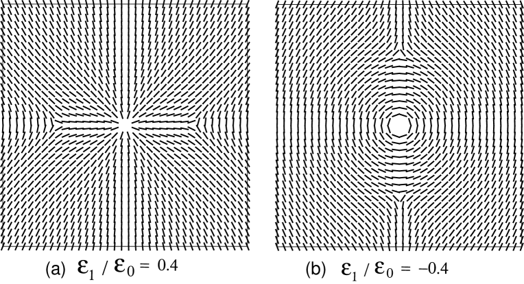
Figure 2: The director in two dimensions for $\varepsilon_{1}/\varepsilon_{0}=0.4$ in (a) and for $\varepsilon_{1}/\varepsilon_{0}=-0.4$ in (b) near the origin. It tends to be along the $y$ axis (in the vertical direction) far from the origin. The spacing between the adjacent bars is $2\ell_{\rm B}$.

and (10) in two dimensions by assuming ${\mbox{\boldmath$n$}}=(\cos\theta,\sin\theta)$ (or $n_{z}=0$). A charge is placed in the hard-core region $(x^{2}+y^{2})^{1/2}<R$. In three dimensions this is the case of an infinitely long charged wire with radius $R$ and charge density $\sigma$, in which all the quantities depend only on $x$ and $y$. The solution can be characterized by the three normalized quantities, $\varepsilon_{1}/\varepsilon_{0}$, $\sigma^{*}\equiv\sigma/(\varepsilon_{0}K)^{1/2}$, and $R/\ell_{\rm B}$. Here we set $\sigma^{*}=2.4$ and $R/\ell_{\rm B}=2$. We discretize the space into a $200\times 200$ lattice in units of $\ell_{\rm B}$ under the periodic boundary condition in the $x$ direction, so the system width is $L=200\ell_{\rm B}$. The electric potential vanishes at $y=0$ and $L$. In Fig.2, $n$ tends to be parallel to the $y$ axis far from the origin and the spacing between the adjacent bars is $2\ell_{\rm B}$. The director is in the radial direction for $\varepsilon_{1}/\varepsilon_{0}=0.4$ in (a) and is perpendicular to $r$ for $\varepsilon_{1}/\varepsilon_{0}=-0.4$ in (b) near the origin. A pair of defects are aligned in the $x$ direction in (a) and in the $y$ direction in (b). Similar defect formation was numerically realized in two dimensions for a neutral particle with the surface interaction (26) below [9, 10].

5 Charged colloidal suspension

The nematic orientation around a large particle without charges[3, 4] is determined by competition of the Frank free energy $F_{0}$ and a microscopic anchoring interaction at the particle surface expressed as

$$F_{\rm a}=-\frac{1}{2}W_{\rm a}\int dS({\mbox{\boldmath$n$}}\cdot{\hat{\mbox{\boldmath$r$}}})^{2}.$$ (26)

Here $\int dS$ is the surface integration, and ${\hat{\mbox{\boldmath$r$}}}$ is the normal unit vector at the surface. The degree of anchoring is represented by the dimensionless parameter,

$$\mu_{\rm a}=W_{\rm a}R/K.$$ (27)

In charged colloidal suspensions, the distortion of $n$ due to the surface charge can be more important than that due to the anchoring interaction (26). Note that (24) is well satisfied even for large $R$ if the ratio $Z/R$ can be increased with increasing $R$. Notice that the ionizable points on the surface is proportional to the surface area $4\pi R^{2}$. However, the problem is very complex, because the counterions themselves can induce large deformation of the nematic order (because of their small size) and tend to accumulate near the large particles.

For simplicity let the deformation of $n$ around the counterions be weak. Furthermore, we assume that the screening length $\lambda$ is shorter than $R$ and the nematic order does not vary on the spacial scale of $\lambda$ except for the defect-core regions. @ Then $F_{\rm e}$ is approximated from (20) as $F_{\rm e}\cong-W_{\rm e}\int dS({\mbox{\boldmath$n$}}\cdot{\hat{\mbox{\boldmath$r$}}})^{2}/2$ with

$$W_{\rm e}={\varepsilon_{1}Z^{2}e^{2}\lambda}/{4\pi\varepsilon_{0}^{2}}R^{4}.$$ (28)

This is of the same form as $F_{\rm a}$ in (26) and the strength of anchoring is represented by $\mu_{\rm eff}=(W_{\rm a}+W_{\rm e})R/K$. Here the Debye-H$\rm{\ddot{u}}$ckel screening becomes extended in the dilute limit. In such cases and in the limit of large $Z/R$, the electric field around a large particle decays on the spatial scale of the Gouy-Chapman length[11],

$$\lambda=k_{\rm B}T/eE_{\rm s}=R^{2}/\ell_{\rm B}Z,$$ (29)

where $E_{\rm s}=Ze/4\pi\varepsilon_{0}R^{2}$ is the electric field at the surface. If $\ell_{\rm B}Z/R\gg 1$, we surely have $\lambda\ll R$. Then we obtain $W_{\rm e}=({\varepsilon_{1}k_{\rm B}T}/{4\pi\varepsilon_{0}})Z/R^{2}$ and

$$\mu_{\rm eff}=(W_{\rm a}/K)R+({\varepsilon_{1}k_{\rm B}T}/{4\pi\varepsilon_{0}}K)Z/R.$$ (30)

The strong anchoring condition is now $|\mu_{\rm eff}|>1$.

6 Concluding remarks

In Section 2, we have presented a scheme of Ginzburg-Landau theory for the electric field effects in liquid crystals, where the dielectric tensor depends on the orientation order as in (3). Generalizations to more complex situations such as ferroelectric cases are straightforward. In Section 3, the director fluctuations have been examined in applied electric field for arbitrary strength of the dielectric anisotropy. It is desirable if (17) could be confirmed by light scattering experiments in systems with not small $\varepsilon_{1}/\varepsilon_{0}$. In Sections 4 and 5, the distortion of the nematic order around a charged particle has been studied for the first time. The condition of strong orientation deformation due to the charge effect is given by (24) if the charge is not screened in the range $r<\ell$ with $\ell$ being defined by (23). In colloidal suspensions the presence of the counterions makes the problem very complex, where we have obtained (30) for the case in which the colloid surface charges are screened within a thin layer with thickness $\lambda\ll R$.

We finally mention a similar charge effect recently predicted for a near-critical polar binary mixture[1]. In such fluids the dielectric constant $\varepsilon(c)$ strongly depends on the composition $c$ and, as a result, the phase separation behavior is strongly affected by doped ions. In particular, if charged colloid particles are suspended, a charge-density-wave phase should be realized for $(|\varepsilon_{1}|/4\varepsilon_{0})Z/R>(\pi C_{0}/\ell_{\rm B})^{1/2}$ at low temperatures, where $\varepsilon_{1}=\partial\varepsilon(c)/\partial c$ and $C_{0}$ is a microscopic wave number($=$the coefficient in the gradient free energy). Here large size of $(|\varepsilon_{1}|/\varepsilon_{0})Z/R$ is required as in (24).

This work is supported by Grants in Aid for Scientific Research from the Ministry of Education, Science, Sports and Culture of Japan.

Appendix
We connect two capacitors in parallel as in Fig.1b. One contains an inhomogeneous dielectric material under investigation and the other is a large capacitor serving as a charge reservoir. The area $S_{0}$ and the charge ${Q}_{0}$ of the large capacitor are much larger than $S$ and ${Q}$ of the smaller capacitor, respectively. We are supposing an experiment in which the total charge ${Q}_{\rm tot}={Q}_{0}+{Q}$ is fixed and the potential difference is commonly given by $\Phi={Q}_{0}/C_{0}$, where $C_{0}$ is the capacitance of the large capacitor. Obviously, in the limit ${Q}/{Q}_{0}\sim S/S_{0}\rightarrow 0$, the deviation of $\Phi$ from the upper bound $\Phi_{\rm tot}={Q}_{\rm tot}/C_{0}$ becomes negligible. Because the electrostatic energy of the large capacitor is given by $E_{0}={Q}_{0}^{2}/2C_{0}=({Q}_{\rm tot}^{2}/2C_{0})(1-{Q}/{Q}_{\rm tot})^{2}$, we obtain

$$E_{0}\cong({Q}_{\rm tot}^{2}/2C_{0})-\Phi{Q},$$ (A.1)

where the first term is constant and a term of order $({Q}/{Q}_{\rm tot})^{2}$ is neglected. Therefore, for the total system including the two capacitors, the relevant free energy is given by $G$ in (11).

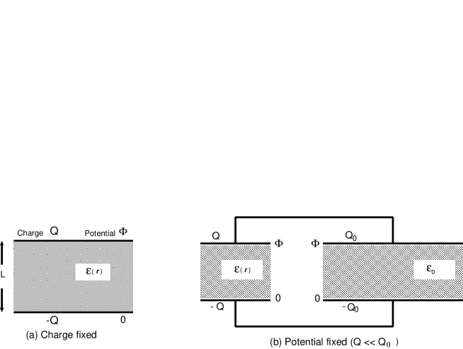
Figure 1: (a) System of a capacitor and an inhomogeneous dielectric material at fixed capacitor charge $Q$. The potential difference $\Phi$ is a fluctuating quantity. (b) Two capacitors connected in parallel with charges ${Q}$ and ${Q}_{0}$. The smaller one contains an inhomogeneous dielectric material, and the larger one a homogeneous dielectric material. In the limit ${Q}/{Q}_{0}\rightarrow 0$, the potential difference $\Phi$ becomes fixed, while $Q$ is a fluctuating quantity.

References

- [1] A. Onuki, in Nonlinear Dielectric Phenomena in Complex Liquids (NATO series) (Kluwer, 2003).
- [2] P.G. de Gennes and J. Prost, The Physics of Liquid Crystals (Oxford, 1993).
- [3] E. M. Terentjev, Phys. Rev. E 51, 1330 (1995).
- [4] P. Poulin, H. Stark, T. C. Lubensky,snd D. A. Weitz, Science 275 1770 (1997).
- [5] R.B. Meyer, Phys. Rev. Lett. 5, 918 (1969).
- [6] L.D. Landau and E.M. Lifshitz, Electrodynamics of Continuous Media (Pergamon, 1984), Chap II.
- [7] M. Born, Z. Phys. 1, 45 (1920).
- [8] J.N. Israelachvili, Intermolecular and Surface Forces (Academic, 1985).
- [9] J. Fukuda and H. Yokoyama, Eur. Phys. E 4, 389 (2001).
- [10] R. Yamamoto, Phys. Rev. Lett. 87, 075502 (2001).
- [11] A.G. Moreira and R.R. Netz, Europhys. Lett. 52, 705 (2000).