Amplitudes for magnon scattering by vortices
in two–dimensional weakly easy–plane ferromagnets

Abstract

We study magnon modes in the presence of a vortex in a circular easy–plane ferromagnet. The problem of vortex–magnon scattering is investigated for partial modes with different values of the azimuthal quantum number $m$ over a wide range of wave numbers. The analysis was done by combining analytical and numerical calculations in the continuum limit with numerical diagonalization of adequately large discrete systems. The general laws governing vortex–magnon interactions are established. We give simple physical explanations of the scattering results: the splitting of doublets for the modes with opposite signs of $m$, which takes place for the long wavelength limit, is an analogue of the Zeeman splitting in the effective magnetic field of the vortex. A singular behavior for the scattering amplitude, $\sigma_{m}\propto k$, takes place as $k$ diverges; it corresponds to the generalized Levinson theorem and can be explained by the singular behavior of the effective magnetic field at the origin.

I Introduction

It is now firmly established that vortices play an important role in the condensed matter physics of two–dimensional (2D) systems with continuously degenerate ground states. In particular, the presence of vortices in 2D easy–plane (EP) magnets gives rise to the Berezinskiĭ–Kosterlitz–Thouless phase transition. Berezinskiĭ (1972); Kosterlitz and Thouless (1973); Kosterlitz (1974) Vortices play an essential role in the thermal and dynamical properties of 2D magnets, for a review see Ref. Mertens and Bishop, 2000. A vortex signature in dynamical response functions can be observed experimentally; e.g. translational motion of vortices leads to a central peak in the dynamical correlation functions. Wiesler et al. (1989) This peak had been predicted predicted both by a vortex gas theory and by combined Monte Carlo – spin dynamics simulations. Mertens et al. (1989)

Recently there has been renewed attention to the problem of magnetic vortices for finite-size magnetic particles, especially their dynamics. It becomes very important in connection with novel composite magnetic materials such as magnetic dot arrays. Thurn-Albrecht et al. (2000); Cowburn and Welland (2000); Shinjo et al. (2000); Sun et al. (2000); Demokritov et al. (2001); Erdin et al. (2002); Cowburn (2002) These magnetic dots are submicron–sized islands made from soft magnetic materials on a nonmagnetic substrate. They are important from a practical standpoint as high–density magnetic storage devices, Grimsditch et al. (2000) and are interesting as fundamentally new objects in the basic physics of magnetism. The distribution of magnetization in such a dot is quite nontrivial: when the dot size is above a critical value, an inhomogeneous state with an out–of plane magnetic vortex occurs, which is stable due to competition between exchange and dipole interactions. Hubert and Shäfer (1998) It is expected that these nonuniform states will drastically change the dynamic and static properties of a dot in comparison with a uniformly magnetized magnetic disk.Recent experiments Novosad et al. (2002); Park et al. (2003) verify such properties; in particular, a mode with anomalously low frequency was detected,Park et al. (2003) see also Refs. Guslienko et al., 2002; Ivanov and Zaspel, 2002.

The general properties of vortex dynamics are intimately connected to the problem of vortex–magnon interactions. Usually this problem has been studied numerically for discrete models, mainly for circular samples cut from large lattice systems. Wysin (1994); Wysin and Völkel (1995, 1996); Wysin (1996); Ivanov et al. (1998); Wysin (2001); Kovalev et al. (2003); Zagorodny et al. (2003) An analytical description of the problem in the framework of the continuum model has been proposed recently for different 2D magnets. Ivanov (1995); Ivanov et al. (1998, 1999); Sheka et al. (2001); Ivanov and Wysin (2002) The most important effect of the vortex–magnon interaction is an excitation of certain magnon modes due to vortex motion and vice versa. Because the magnons in the EP ferromagnet have a gapless dispersion law, a possible Larmor dynamics of the vortex center is strongly coupled with a magnon cloud; Kovalev et al. (2003) therefore the corresponding motion has a non–Newtonian form. Ivanov et al. (1998)

In this paper we consider the magnon modes which exist in a 2D Heisenberg EP ferromagnet in the presence of a vortex. We apply different, sometimes new, methods of analytical and numerical investigation, in order to extend the research of Ref. Ivanov et al., 1998, presenting a wider range of results for the magnon scattering amplitude. In Sec. II we demonstrate that the vortex acts on magnons in two ways. First of all, it provides for coupling between different directions of magnetization precession; the magnon modes are described by a “generalized” Schrödinger equation. Secondly, the problem naturally possesses an effective magnetic field, whose global properties are caused by the soliton topological charge. The scattering problem is treated both numerically and analytically for a wide range of wave numbers. The numerical study is carried out using two different approaches: solving the eigenvalue problem for the continuum limit (in the weak EP anisotropy limit), and extracting the scattering data from numerical diagonalization of discrete systems, see Sec. III. The analytical study of the scattering problem is developed (Sec. IV) using both the long– and short–wavelength approximations. In contrast to the previous work Ivanov et al. (1998) we describe analytically the splitting phenomenon of the doublets of magnon modes with opposite signs of the azimuthal quantum number, and give a physical picture of this effect: an effective magnetic field causes the Zeeman splitting of the magnon levels, see Sec. IV.1. The singular behavior of the scattering amplitude is predicted in Sec. IV.2 for the short wavelength limit. This feature is caused by the specific singular effective magnetic field at the origin (vortex core); this study verifies the generalized version of the Levinson theorem, which we have established recently in Ref. Sheka et al., 2003 for potentials with inverse square singularities.

II Model and magnon modes

We consider the classical 2D Heisenberg ferromagnet (FM) with the Hamiltonian

$$\mathcal{H}=-J\sum_{\left(\bm{n},\bm{n}^{\prime}\right)}\left[\bm{S}_{\bm{n}}\cdot\bm{S}_{\bm{n}^{\prime}}-(1-\lambda){S}_{\bm{n}}^{z}{S}_{\bm{n}^{\prime}}^{z}\right],$$ (1)

where the spins $\bm{S}_{\bm{n}}$ are classical vectors on a square lattice with the lattice constant $a$. Here $\left(\bm{n},\bm{n}^{\prime}\right)$ denotes nearest–neighbor lattice sites, $J>0$ is the exchange integral, and $\lambda\in[0,1)$ describes easy–plane anisotropy.

We consider the continuum dynamics of the Heisenberg ferromagnet, which is adequate for model (1) in the small–anisotropy case ($1-\lambda\ll 1$). In a continuum limit the dynamics of the FM is described by Landau–Lifshitz equations for the normalized magnetization,

$$\bm{m}(\bm{r},t)=\frac{\bm{S}(\bm{r},t)}{S}=\Bigl{(}\sin\theta\cos\phi;\sin\theta\sin\phi;\cos\theta\Bigr{)}.$$ (2)

The equations of motion result from the Lagrangian

$$L=\frac{S}{a^{2}}\int\text{d}^{2}x(1-\cos\theta)\frac{\partial\phi}{\partial t}-E[\theta,\phi],$$ (3)

with the energy functional

$$E[\theta,\phi]=\frac{JS^{2}}{2}\!\!\int\!\!\text{d}^{2}x\!\left[\left(\nabla\theta\right)^{2}+\left(\nabla\phi\right)^{2}\sin^{2}\theta+\frac{\cos^{2}\theta}{r_{v}^{2}}\right].$$ (4)

Here $r_{v}=\frac{a}{2}\sqrt{\lambda/(1-\lambda)}$ is the characteristic length scale (“magnetic length”). One should note that the strength of the weak easy-plane anisotropy ($\lambda\approx 1$), determines the magnetic length scale $r_{v}$; in this continuum analysis, results will depend on lengths scaled by $r_{v}$, and have no explicit dependence on the anisotropy strength.

The ground state of the magnet is continuously degenerate and isotropic within the easy plane (EP). The simplest elementary linear excitations of EP FMs that arise on the homogeneous background are the magnons belonging to a continuous spectrum. They have the form of elliptically polarized waves; if one chooses the homogenous spin distribution along the $x$–axis, then the spin wave takes the form:

$$m_{x}=1,\quad m_{z}+{i}m_{y}\cdot\frac{kr_{v}}{\sqrt{1+k^{2}r_{v}^{2}}}\propto\exp({i}kx-{i}\omega t).$$ (5)

The dispersion law has the gapless form:

$$\omega(\bm{k})=ck\sqrt{1+k^{2}r_{v}^{2}},$$ (6)

where $c=2aJS\sqrt{1-\lambda}$ is the characteristic magnon speed, $\bm{k}$ is the magnon wave vector, and $k=|\bm{k}|$ is its magnitude.

The simplest nonlinear excitation in the system is an out–of–plane (OP) vortex Gouvêa et al. (1989); Kosevich et al. (1990)

$$\begin{split}&\phi\equiv\phi_{0}=\varphi_{0}+q\chi,\quad\theta=\theta_{0}(\rho),\\ &\theta_{0}(0)=\frac{1-p}{2}\pi,\quad\theta_{0}(\infty)=\pi/2,\end{split}$$ (7)

where $\varphi_{0}$ is an arbitrary angle due to the EP symmetry, $\rho\equiv|\bm{r}|/r_{v}$ and $\chi$ are dimensionless polar coordinates in the plane of the magnet, the vorticity $q\in\mathbb{Z}$ plays the role of a $\pi_{1}$ topological charge, and the polarization $p=\pm 1$ is connected with a $\pi_{2}$ topological charge (the Pontryagin index):

$$Q=\frac{1}{4\pi}\int\mathcal{Q}\;\text{d}^{2}x,\qquad\mathcal{Q}=\frac{1}{2}\epsilon_{ij}\ \bm{m}\cdot\left(\partial_{i}\bm{m}\times\partial_{j}\bm{m}\right).$$ (8)

We term $\mathcal{Q}$ the gyrocoupling density, following Thiele (1973); it has a sense as the density of the topological charge, see Papanicolaou and Tomaras (1991). For the vortex configuration (7) the gyrocoupling density can be represented as

$$\mathcal{Q}=\frac{q\sin\theta_{0}\cdot\theta_{0}^{\prime}}{\rho},$$ (9)

hence the Pontryagin index takes on half–integer or integer values $Q=qp/2$. Note that the presence of a nontrivial $\pi_{2}$–topological charge directly results in the gyrotropical dynamics of the vortex, which conserves the gyrovector $\bm{G}=Q\cdot 2\pi\hslash Sa^{-2}\bm{e}_{z}$.

The function $\theta_{0}$ is the solution of an ordinary differential equation, which can only be solved numerically. Kosevich et al. (1990); Bar’yakhtar and Ivanov (1993) Without an external magnetic field two oppositely polarized vortices are energetically equivalent; for definiteness we set $p=+1$.

To analyze magnons on the vortex background, we use a formalism and set of coordinates developed in Ref. Wysin and Völkel, 1995, setting up the problem in terms of local Cartesian spin components. The unperturbed spins of the static vortex structure, $\bm{m}_{0}$, define local polar axes $\bm{e}_{3}$, different at every site, specifically, $\bm{S}_{0}(\bm{r},t)=S\bm{e}_{3}$.

It is to be understood that these axes depend on the site chosen. The magnetic fluctuations occur perpendicular to these local axes, suggesting the definition of other axes, $\bm{e}_{2}$ being chosen along the direction of $\bm{e}_{z}\times\bm{e}_{3}$, and $\bm{e}_{1}=\bm{e}_{2}\times\bm{e}_{3}$, to complete the mutually perpendicular set. One supposes that a dynamically fluctuating spin has small deviations along the $\bm{e}_{1}$ and $\bm{e}_{2}$ axes so that a spin is written as

$$\bm{S}(\bm{r},t)=S\left(\bm{e}_{3}+m_{1}\bm{e}_{1}+m_{2}\bm{e}_{2}\right).$$ (10)

The fields $m_{1}$ and $m_{2}$ have a simple physical significance, which can be seen if a given spin is supposed to have small deviations $\varphi$ and $\vartheta$ away from the vortex structure, determined by azimuthal and polar spherical angles, $\phi_{0}$ and $\theta_{0}$. We write

$$\begin{split}\frac{\bm{S}(\bm{r},t)}{S}&=\cos(\theta_{0}+\vartheta)\bm{e}_{z}+\sin(\theta_{0}+\vartheta)\\ &\times\left[\cos(\phi_{0}+\varphi)\bm{e}_{x}+\sin(\phi_{0}+\varphi)\bm{e}_{y}\right].\end{split}$$ (11)

Linearizing in $\varphi$ and $\vartheta$, and using the definitions of $\{\bm{e}_{1},\bm{e}_{2},\bm{e}_{3}\}$, comparison of Eqs. (10) and (11) shows that

$$m_{1}=\vartheta,\quad m_{2}=\varphi\sin\theta_{0}.$$ (12)

Thus, the $m_{1}$ field measures spin rotations moving towards the polar ($\bm{e}_{z}$) axis and the $m_{2}$ field measures spin rotations projected onto the $xy$–plane. In the absence of the vortex, we have $\theta_{0}=\pi/2$, $\phi_{0}=0$, and such oscillations correspond to the free magnons in the form (5).

The linearized equations for $m_{1}$ and $m_{2}$ can be described by a single complex–valued function $\psi(\bm{r},t)=m_{1}+{i}m_{2}$, which obeys the differential equation

$${i}\partial_{\tau}\psi=H\psi+W\psi^{*},\qquad H=\left(-{i}\bm{\nabla}-\bm{A}\right)^{2}+U,$$ (13)

with the “potentials”

$$U(\rho) = \frac{1}{2}\sin^{2}\theta_{0}\left(1-\frac{q^{2}}{\rho^{2}}\right)-\cos^{2}\theta_{0}-\frac{{\theta^{\prime}_{0}}^{2}}{2},$$ (14a)

$$W(\rho) = \frac{1}{2}\sin^{2}\theta_{0}\left(1-\frac{q^{2}}{\rho^{2}}\right)+\frac{{\theta^{\prime}_{0}}^{2}}{2},$$ (14b)

$$\bm{A}(\rho) = -\frac{q\cos\theta_{0}}{\rho}\cdot\bm{e}_{\chi}.$$ (14c)

Here we use the dimensionless coordinate variable $\rho=|\bm{r}|/r_{v}$, dimensionless time variable $\tau=t\cdot c/r_{v}$, and the operator $\bm{\nabla}=r_{v}\partial_{\bm{r}}$; prime denotes $\text{d}/\text{d}\rho$.

Let us note that the vector $\bm{A}$ acts in the Schrödinger–like operator $H$ in the same way as the vector–potential acts in the Hamiltonian of a charged particle. Then it is possible to conclude that there is an effective magnetic flux density

$$\bm{B}=\bm{\nabla}\times\bm{A}=\bm{e}_{z}\cdot\frac{q\sin\theta_{0}\cdot\theta^{\prime}_{0}}{\rho}.$$ (15)

Note that the effective magnetic flux density can easily be rewritten through the gyrocoupling density (9) as $\bm{B}=\mathcal{Q}\cdot\bm{e}_{z}$. Therefore the total flux is determined by the nontrivial $\pi_{2}$ topology of the vortex configuration. On first view when exploiting this analogy it is possible to look for the Aharonov–Bohm phenomenon for the scattering problem, because this magnetic flux density is localized in the region of the vortex core. However, one can see that the total magnetic flux

$$\Phi=\int B_{z}\text{d}^{2}x=4\pi Q=qp\Phi_{0}$$ (16)

is an integer multiple of the flux quantum $\Phi_{0}=2\pi$, so there is no Aharonov–Bohm scattering picture for the system.

A differential equation like (13) is not a unique property of the vortex–magnon problem in the EP FM only. It appears for different kinds of anisotropy: it describes magnon modes on the soliton background in the easy–axis Sheka et al. (2001) and isotropic magnets Ivanov et al. (1999). Note that for the specific case of an isotropic system with an exact analytical soliton solution of the Belavin–Polyakov type, the potential $W$ disappears, so the magnon modes satisfy the usual Schrödinger like equation ${i}\partial_{\tau}\psi=H\psi$, which describes, e.g., the quantum mechanical states for a charged particle in the axially symmetric potential $U(\rho)$ under the action of an external magnetic field with a vector potential $\bm{A}$.

For the anisotropic case, when $W\neq 0$, the problem (13) has important unusual properties, which are absent for the Belavin–Polyakov case. More generally, there appear properties which are forbidden for the usual quantum mechanics. In particular, an effective discrete Hamiltonian of the system is not necessarily Hermitian; in Refs. Wysin and Völkel, 1995, 1996; Wysin, 2001 some constructive methods were elaborated to avoid these problems. Nevertheless we will discuss the features of Eq. (13) in order to understand why the standard quantum mechanical intuition could fail.

The standard quantum mechanical equation ${i}\partial_{\tau}\psi=H\psi$ allows the conservation law $\partial_{\tau}|\psi|^{2}=-\bm{\nabla}\cdot\bm{j}$ for the current

$$\bm{j}={i}\left(\psi\bm{\nabla}\psi^{*}-\psi^{\star}\bm{\nabla}\psi\right)+2|\psi|^{2}\bm{A}.$$ (17)

The generalized Schrödinger–like equation (13) with $W\neq 0$ violates this conservation law, namely:

$$\partial_{\tau}|\psi|^{2}=-\bm{\nabla}\cdot\bm{j}-{i}W\left({\psi^{*}}^{2}-\psi^{2}\right).$$ (18)

Nonconservation of probability density has posed some problems in the passage from standard quantum mechanics to old pre–Feynmann quantum electrodynamics. The reason is that Eq. (13) is formulated neither for a Hermitian, nor a linear operator; the last statement is due to the broken symmetry under the rescaling $\psi\to\lambda\psi$ with $\lambda\in\mathbb{C}$. There exists an analogy with relativistic theory: there can appear solutions with positive and negative energy in the passage from the Klein–Gordon to Dirac equation. In fact, our problem has the same origin. Let us reformulate the problem (13) as an equation second order in time. One can calculate that the Klein–Gordon–like equation

$$-\partial_{\tau\tau}\psi=\left(H^{2}-W^{2}\right)\psi$$ (19)

is valid far from the vortex center. What is important is that Eq. (19) contains a Hermitian operator (similar arguments were used in Ref. Wysin, 2001). Therefore, the eigenvalue problem (EVP) for $\omega^{2}$, not for $\omega$, is more appropriate for this system; the only problem is to separate solutions with positive and negative $\omega$. Note, that there appear $4^{\rm th}$ order operators with respect to the space coordinate, which causes the presence of master and slave functions in the solution, see below.

Such a problem, as well as a problem with nonconserved number of particles (probability amplitude), appears in the theory of a weakly nonideal Bose gas. It results, in fact, in the separation of positive and negative energy solutions under u–v Bogolyubov transformations. Lifshitz and Pitaevsky (1999)

Following this scheme we need to generalize the u–v transformation to the nonhomogeneous case.

We apply the partial–wave expansion, using the ansatz Ivanov et al. (1998)

$$\begin{split}\psi(\bm{r},t)&=\sum_{\alpha}\left[u_{\alpha}(\rho)e^{{i}\Phi_{\alpha}}+v_{\alpha}(\rho)e^{-{i}\Phi_{\alpha}}\right],\\ \Phi_{\alpha}(\chi,t)&=m\chi-\omega_{\alpha}t+\eta_{m}=m\chi-\varOmega_{\alpha}\tau+\eta_{m},\end{split}$$ (20)

where $\alpha=(k,m)$ is a full set of eigenvalues, $m\in\mathbb{Z}$ being azimuthal quantum numbers, the $\eta_{m}$ are arbitrary phases, and $\varOmega=\omega r_{v}/c$ are dimensionless frequencies. This expansion leads to the following EVP for the radial eigenfunctions $u$ and $v$ (the index $\alpha$ will be omitted in the following):

$$\textsf{H}\bm{\bigl{|}\varPsi\bigr{>}}=\varOmega\bm{\bigl{|}\varPsi\bigr{>}},\;\textsf{H}=\begin{Vmatrix}H_{+}&W\\ -W&-H_{-}\\ \end{Vmatrix},\;\bm{\bigl{|}\varPsi\bigr{>}}=\begin{Vmatrix}u\\ v\end{Vmatrix}.$$ (21)

Here $H_{\pm}=-\nabla_{\rho}^{2}+\mathcal{U}_{0}+1/2\pm V$ is the 2D radial Schrödinger–like operator with the “potentials”

$$\mathcal{U}_{0}(\rho)=U(\rho)+\bm{A}^{2}+\frac{m^{2}}{\rho^{2}}-\frac{1}{2}$$

$$=\frac{q^{2}+m^{2}}{\rho^{2}}-\frac{3q^{2}\sin^{2}\theta_{0}}{2\rho^{2}}-\frac{3\cos^{2}\theta_{0}}{2}-\frac{{\theta^{\prime}_{0}}^{2}}{2},$$ (22)

$$V(\rho)=-\frac{2m\left(\bm{A}\cdot\bm{e}_{\chi}\right)}{\rho}=\frac{2qm\cos\theta_{0}}{\rho^{2}},$$ (23)

$\nabla_{\rho}^{2}=\text{d}^{2}/\text{d}\rho^{2}+(1/\rho)\text{d}/\text{d}\rho$ is the radial Laplace operator. In spite of the fact that the EVP (21) is formulated for the Schrödinger operators $H_{\pm}$, this EVP is different in principle from the usual set of coupled Schrödinger equations, which is widely used, e.g. for the description of multichannel scattering. Newton (1982) The reason is that the matrix Hamiltonian H is not Hermitian for the standard metric, for details see Ref. Wysin, 2001. To avoid this problem we introduce a corresponding bra–vector by the definition

$$\bm{\bigl{<}\varPsi\bigl{|}}=\bigl{\|}u\;;-v\bigr{\|}.$$ (24)

The Hilbert space for the $\bm{\varPsi}$–function has an indefinite metric,

$$\bm{\bigl{<}\varPsi\bigr{|}\varPsi\bigr{>}}=(u|u)-(v|v),$$ (25)

where $(u|v)=\int_{0}^{\infty}u(\rho)v(\rho)\rho\text{d}\rho$ is the standard scalar product. By introducing such a Hermitian product, it is possible to define the standard energy functional, cp. Ref. Sheka et al., 2001:

$$\mathcal{E}[u,v]=\bm{\bigl{<}\varPsi\bigl{|}\textsf{H}\bigr{|}\varPsi\bigr{>}}=(u|H_{+}|u)+2(u|W|v)+(v|H_{-}|v).$$ (26)

Let us mention that Eq. (21) is invariant under the conjugations $\varOmega\to-\varOmega$, $m\to-m$, and $u\leftrightarrow v$. In a classical theory we can choose either sign of the frequency; but in order to make contact with quantum theory, with a positive frequency and energy $\mathcal{E}_{k}=\hslash\omega_{k}$, we will discuss the case $\varOmega>0$ ($\omega>0$) only. Thus there are two different equations for the opposite signs of $m$. However, in the limiting case of the “zero modes” with $\varOmega=0$, the system again is invariant under conjugations $m\to-m$. For example, one of the zero modes, the so–called translational mode with $m=+1$, has the form

$$u_{m=+1}=\frac{\sin\theta_{0}}{\rho}-\theta^{\prime}_{0},\qquad v_{m=+1}=\frac{\sin\theta_{0}}{\rho}+\theta^{\prime}_{0},$$ (27)

which describes the position shift of the soliton. Because of the degeneration of the EVP at $\varOmega=0$, it leads to the existence of a zero mode with $m=-1$; the eigenfunction of this mode can be expressed just from (27) under the conjugation $u\leftrightarrow v$. We use here notations for mode indices as in Refs. Ivanov et al., 1999; Ivanov and Wysin, 2002; note that the mode with $m=+1$ corresponds in our notation to the mode with $m=-1$ in the notations of Refs. Ivanov et al., 1998; Sheka et al., 2001.

It should be stressed that the picture is quite different for the special case $W=0$, which corresponds to the isotropic magnet. Ivanov (1995); Ivanov et al. (1999) Here we have two uncoupled equations for the functions $u$ and $v$. One of the equations (for the eigenfunction $v$) has the negative eigenvalue $-\varOmega$, from which it necessarily results that $v\equiv 0$. In this special case the zero modes (27) have the form $u_{+1}\propto\theta_{0}^{\prime}$ and $v_{+1}=0$. Therefore the zero mode with $m=-1$ cannot be obtained by the simple conjugation. It explains the difference between the collective dynamics of the soliton in isotropic magnets, where it is enough to take into account only the mode with $m=+1$, and the EP FM, where translational modes with $m=-1$ and $m=+1$ must be taken into account. Nevertheless, the roles of the modes with $m=-1$ and $m=+1$ are not equal, for details see Sec. IV.3.

III Scattering problem: numerical results

III.1 Continuum approach

We intend to describe the scattering of magnons by a vortex. However the EVP (21) is not adjusted for the scattering problem, because it does not provide the asymptotic independence of the equations at infinity. To solve the problem it is convenient to make a unitary transformation of the eigenvector $\bm{\bigl{|}\varPsi\bigr{>}}$,

$$\bm{\bigl{|}\widetilde{\varPsi}\bigr{>}}=\textsf{A}\bm{\bigl{|}\varPsi\bigr{>}},\quad\textsf{A}=\begin{Vmatrix}\cos\varepsilon&-\sin\varepsilon\\ \sin\varepsilon&\cos\varepsilon\\ \end{Vmatrix},\;\bm{\bigl{|}\widetilde{\varPsi}\bigr{>}}=\begin{Vmatrix}\tilde{u}\\ \tilde{v}\end{Vmatrix}.$$ (28)

The angle $\varepsilon$ of this unitary transformation is defined by the expression

$$\tan 2\varepsilon=\frac{1}{2\varOmega}.$$ (29)

Then we obtain the following partial differential equation for the function $\bm{\bigl{|}\widetilde{\varPsi}\bigr{>}}$:

$$\widetilde{\textsf{H}}\bm{\bigl{|}\widetilde{\varPsi}\bigr{>}}=\bm{\Lambda}\bm{\bigl{|}\widetilde{\varPsi}\bigr{>}},\;\widetilde{\textsf{H}}=\textsf{H}_{0}+\widetilde{\textsf{V}},\;\bm{\Lambda}=\text{diag}\left(\kappa^{2};\varkappa^{2}\right),$$ (30a)

$$\textsf{H}_{0}=\text{diag}\left(\mathcal{H}_{0};-\mathcal{H}_{0}\right),\quad\mathcal{H}_{0}=-\nabla_{\rho}^{2}+\mathcal{U}_{0},$$ (30b)

$$\widetilde{\textsf{V}}=\left[V+\bm{g}\cdot\left(W-1/2\right)\right]\textsf{A}^{-2},$$ (30c)

where $\bm{g}=\bigl{\|}\begin{smallmatrix}0&1\\ -1&0\end{smallmatrix}\bigr{\|}$ is a metric spinor, the dimensionless wave number is $\kappa=kr_{v}$, and $\varkappa=\sqrt{\kappa^{2}+1}$.

First let us consider the magnon spectrum in the absence of a vortex (free fields). Without a vortex ($q=0$, $\theta_{0}=\pi/2$), Eqs. (30) are uncoupled, which results in free magnons,

$$\begin{split}\tilde{u}_{m}(\rho)&\propto J_{|m|}(\kappa\rho)\underset{\kappa\rho\gg 1}{\sim}\sqrt{\frac{2}{\pi\kappa\rho}}\cdot\cos\left(\kappa\rho-\frac{|m|\pi}{2}-\frac{\pi}{4}\right),\\ \tilde{v}_{m}(\rho)&=0,\end{split}$$ (31)

where $J_{m}$ are Bessel functions. The free modes $\tilde{u}_{m}$ play the role of the partial cylinder waves of a plane spin wave

$$\exp\left({i}\bm{k}\cdot\bm{r}-{i}\omega t\right)=\sum_{m=-\infty}^{\infty}{i}^{m}J_{m}(\kappa\rho)e^{{i}m\chi-{i}\omega t}.$$ (32)

To describe magnon solutions in the presence of a vortex, one should note that far from the vortex center the potential $\widetilde{\textsf{V}}$ tends to zero, so the Eqs. (30a) become uncoupled,

$$\left(\nabla_{\rho}^{2}+\kappa^{2}\right)\tilde{u}=0,\;\left(\nabla_{\rho}^{2}-\varkappa^{2}\right)\tilde{v}=0,\;\rho\gg\max\left(1;\frac{1}{\kappa};\frac{1}{\varkappa}\right)$$ (33)

with asymptotically independent solutions:

$$\tilde{u}_{m}(\rho) \sim\frac{C_{1}}{\sqrt{\rho}}\cdot e^{{i}\kappa\rho}+\frac{C_{2}}{\sqrt{\rho}}\cdot e^{-{i}\kappa\rho}$$

$$\propto\frac{1}{\sqrt{\rho}}\cos\left(\kappa\rho-\frac{|m|\pi}{2}-\frac{\pi}{4}+\delta_{m}\right),$$ (34a)

$$\tilde{v}_{m}(\rho) \sim\frac{C_{3}}{\sqrt{\rho}}\cdot e^{\varkappa\rho}+\frac{C_{4}}{\sqrt{\rho}}\cdot e^{-\varkappa\rho}.$$ (34b)

The scattering results in the quantity $\delta_{m}\equiv\delta_{m}(\kappa)$; it can be interpreted as the scattering phase shift, determining the intensity of the magnon scattering due to the presence of the vortex. Sometimes it is useful to introduce the scattering amplitude, $\sigma_{m}=-\tan\delta_{m}$. Using this notation, the oscillatory solution (34a) can be rewritten in the following form

$$\tilde{u}_{m}(\rho)\propto J_{|m|}(\kappa\rho)+\sigma_{m}\cdot Y_{|m|}(\kappa\rho).$$ (34a^′)

where $Y_{|m|}$ are Neumann functions. Let us stress that the solution (34a^′) is valid only in the sense of the asymptotic form (34a). As it follows from Eq. (34b), the function $\tilde{v}$ has an exponential behavior,

$$\tilde{v}_{m}(\rho)\propto K_{|m|}(\varkappa\rho)+\gamma_{m}\cdot I_{|m|}(\varkappa\rho)\propto\frac{e^{-\varkappa\rho}}{\sqrt{\rho}}+\gamma_{m}\cdot\frac{e^{\varkappa\rho}}{\sqrt{\rho}},$$ (34b^′)

where $K_{|m|}$ and $I_{|m|}$ are MacDonald and modified Bessel functions, respectively; at the same time $\tilde{u}$ yields oscillatory solutions. Naturally, the real modes have an oscillatory form here; we will use this fact below for the numerical analysis. It means that the function $\tilde{u}$ becomes a master function in the Eq. (30a), while $\tilde{v}$ is a slave (note, that we choose $\varOmega>0$). This mirrors the difference between Eq. (30a) and a usual set of Schrödinger equations.

The scattering amplitude, or, equivalently, the phase shift, contains all information about the scattering processes. In particular, the general solution of the scattering problem for a plane wave can be expressed in the form, cp. Eq. (5)

$$m_{2}-{i}m_{1}\cdot\frac{kr_{v}}{\sqrt{1+k^{2}r_{v}^{2}}}\propto e^{{i}\bm{k}\cdot\bm{r}-{i}\omega t}+\mathcal{F}(\chi)\cdot\frac{e^{{i}\kappa\rho-{i}\omega t}}{\sqrt{\rho}},$$ (35a)

where the scattering function has the form Ivanov et al. (1999)

$$\mathcal{F}(\chi)=\frac{\exp(-{i}\pi/4)}{\sqrt{2\pi\kappa}}\cdot\sum_{m=-\infty}^{\infty}\left(e^{2{i}\delta_{m}}-1\right)\cdot e^{{i}m\chi}.$$ (35b)

The total scattering cross section is given by the expression

$$\varrho=\int_{0}^{2\pi}\!|\mathcal{F}|^{2}\text{d}\chi=\sum_{m=-\infty}^{\infty}\!\varrho_{m}\;,$$

where $\varrho_{m}=(4/k)\sin^{2}\delta_{m}$ are the partial scattering cross sections.

Let us switch to the numerical solution of the scattering problem in the continuum approach. The differential problem to be integrated consists of Eq. (30) and asymptotic conditions at the center of the vortex and at infinity:

$$\widetilde{\textsf{H}}\bm{\bigl{|}\widetilde{\varPsi}\bigr{>}} =\bm{\Lambda}\bm{\bigl{|}\widetilde{\varPsi}\bigr{>}},$$ (36a)

$$\bm{\bigl{|}\widetilde{\varPsi}\bigr{>}} \sim\textsf{A}\cdot\begin{Vmatrix}\epsilon_{m}\cdot\rho^{|m+1|},\\ \rho^{|m-1|}\end{Vmatrix},\qquad\text{when}\;\rho\ll 1$$ (36b)

$$\bm{\bigl{|}\widetilde{\varPsi}\bigr{>}} \sim\begin{Vmatrix}J_{|m|}(\kappa\rho)+\sigma_{m}\cdot Y_{|m|}(\kappa\rho)\\ K_{|m|}(\varkappa\rho)\end{Vmatrix},$$

$$\qquad\text{when}\;\rho\gg\max\left(1;\frac{1}{\kappa};\frac{1}{\varkappa}\right).$$ (36c)

The presence of the matrix A in the condition (36b) means that the functions $\tilde{u}$ and $\tilde{v}$ are not asymptotically independent even in the lowest approximation. In the next approximation there appears an additional “interaction” between $\tilde{u}$ and $\tilde{v}$, which is realized in the nonunit factor $\epsilon_{m}$; its value cannot be found through this asymptotic expansion.

We use the one–parameter shooting method, solving Eqs. (36), as described in Ref. Ivanov et al., 1996; Sheka et al., 2001. Choosing the shooting parameter $\epsilon_{m}$, we “kill” the growing exponent for the function $\tilde{v}_{m}$ in (34b^′), where the coefficient $\gamma_{m}$ should be equal to zero; as a result we have obtained a well–pronounced exponential decay for $\tilde{v}_{m}\propto K_{|m|}(\varkappa\rho)$, and oscillating solutions for $\tilde{u}_{m}$. The scattering amplitude was found from these data by comparison with the asymptotes (36c). The results are discussed in Sec. III.3.

III.2 Discrete approach

In the discrete lattice approach, the small amplitude spin fluctuation modes in the presence of a vortex at the center of a finite circular system of radius $R$ are found. The spins occupy sites on a square lattice. We use the formalism and set of local coordinates as described in Sec. II for the continuum model. Similar to the continuum expression (10), we describe the dynamically fluctuating spin on lattice site $\bm{n}$ as

$$\bm{S}_{\bm{n}}=S\left(\bm{e}_{3}+m_{1}\bm{e}_{1}+m_{2}\bm{e}_{2}\right),$$ (10^′)

where $m_{1}$ and $m_{2}$ measure spin rotations moving towards the polar axis and projected onto the $xy$–plane, respectively, see Eq. (12).

The spin dynamics equations of motion with an assumed $e^{-i\omega t}$ time dependence were linearized in $m_{1}$ and $m_{2}$, leading to an eigenvalue problem requiring numerical diagonalization. We assumed a Dirichlet boundary condition, $m_{1}=m_{2}=0$ at the edge of the system studied. For circular systems of radius $R$, we used a Gauss–Seidel relaxation scheme Wysin (2001) to calculate the frequencies and eigenfunctions of some of the lowest eigenmodes with a single vortex present at the system center. Before doing this, the vortex structure was relaxed to an accurate static structure using an energy minimization scheme. The diagonalization is partial; typically only the lowest 20 to 40 eigenstates were found, which substantially reduces the computing time needed, and relaxes constraints on the precision of the calculations. This limited diagonalization, however, gives only modes which have long wavelength spatial variations, which provides for a good comparison with continuum theory.

We considered different values of $\lambda$ close to $1$. Although the continuum limit would be better represented by using $\lambda$ very close to $1$, this could result in a vortex radius $r_{v}=\frac{a}{2}\sqrt{\lambda/(1-\lambda)}$ easily exceeding the system size that can be treated numerically. Therefore, data were calculated using $\lambda=0.99$, for which $r_{v}\approx 4.97a$. With this size of vortex length scale, discreteness effects due to the underlying lattice should be unimportant, and still, the vortex structure fits well within the confines of a system with a radius as small as $R\approx 10a$, so that finite size effects should also be negligible.

In general, a given mode has $e^{im\chi}$ angular dependence on the azimuthal coordinate $\chi$, where $m$ is some integer azimuthal quantum number. In the continuum theory presented in Sec. II, $m$ is a good quantum number, due to rotational invariance. This symmetry is weakly broken on a lattice, but for long-wavelength and lower frequency modes, $m$ can be considered a good quantum number even on a lattice. (Generally, the calculated magnon wavefunctions were sometimes found to be composed of linear combinations of $+m$ and $-m$ components.) The numerically found modes were also characterized by a principle quantum number $n$, being the number of nodes in the wavefunction along the radial direction. For a mode of determined $m$ and $n$, the scattering amplitude $\sigma$ was found by a fitting procedure applied to the calculated eigenfunction for that mode (essentially, finding the ratio of outgoing and incoming waves), see Ref. Wysin, 2001 for details.

In the continuum theory, scattering was analyzed as a function of wavevector $k$, or in terms of the dimensionless $kr_{v}$. For lattice calculations, the values of $k$ cannot be chosen freely, instead, they are determined by the actual system size. For a mode found to be oscillating at eigenfrequency $\omega$, the wavevector magnitude $k$ associated with the mode was found by supposing $\bm{k}=(k,0)$, and inverting the free magnon dispersion relation for the 2D EP FM on a lattice,

$$\begin{split}\omega_{\bm{k}}&=4JS\sqrt{(1-\gamma_{\bm{k}})(1-\lambda\gamma_{\bm{k}})},\\ \gamma_{\bm{k}}&=\frac{1}{2}(\cos k_{x}+\cos k_{y}).\end{split}$$ (37)

Therefore, a calculation of the modes for a single lattice size gives only specific values of $\kappa=kr_{v}$, one value corresponding to each mode. To get a wider and more continuous range of data for comparison with the continuum theory, calculations were carried out on lattices ranging in radius from $R=15a$ to $R=40a$. By plotting results as functions of $kr_{v}$, for fixed $m$ but from various $n$ and $R$, the data from the different system sizes superimposes smoothly, giving more slowly changing $kr_{v}$, which is more appropriate for comparison with the continuum limit.

III.3 Numerical results

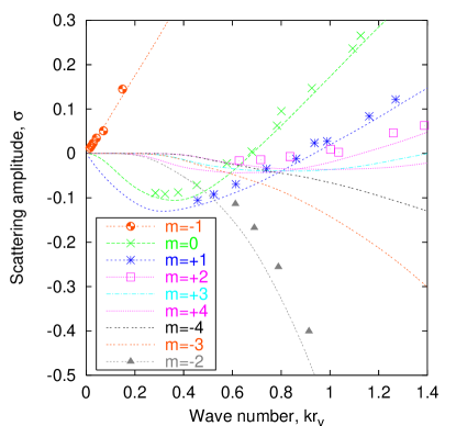
Figure 1: (Color online) Scattering data for different $m$ for small wave numbers, $kr_{v}<1.3$: from continuum theory (lines) and from discrete model numerical diagonalization (symbols) in circular square lattice systems of radii $R=15,20,25,30,35,40$.

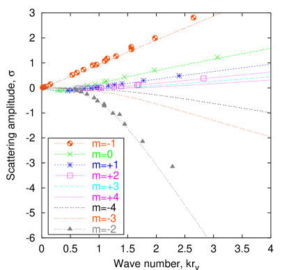
Figure 2: (Color online) Scattering data for different $m$ for a wide region of wave numbers $k$: from continuum theory (lines) and from discrete model numerical diagonalization (symbols).

Numerically, we have obtained the data of the vortex–magnon scattering by the two different approaches discussed above: solving the scattering problem (36) using the shooting method for the continuum limit, and extracting the scattering data from numerical diagonalization of finite discrete systems. To be specific, data are presented for scattering from a vortex with unit vorticity, $q=+1$ and positive polarization, $p=+1$. One should note that results for vortex–magnon scattering for modes $m$ from other vortex types, as seen in Eq. (23), should be depend on the sign of $qpm$. The results are the following:

For all modes the scattering amplitude $\sigma_{m}(k)$ tends to zero as $k\to 0$. In the long–wavelength limit the maximal scattering is related to the modes with $m=\pm 1$. Except for the mode with $m=-1$, the scattering amplitude in the long–wavelength limit takes a negative value, see Fig. 1. At extremely low values of wave number $\kappa\lesssim 0.01$, the scattering data contain sets of doublets for modes with opposite signs of $m$. In the long–wavelength limit the doublet splitting appears as a small correction, but the scattering picture changes when $k$ increases. For all modes $\sigma_{m}(k)$ diverges as $k\to\infty$: the scattering amplitude $\sigma_{m}(k\to\infty)\to+\infty$ for all modes with $m\geq-1$, but $\sigma_{m}(k\to\infty)\to-\infty$ for $m<-1$, see Fig. 2. Naturally, there is no real divergence; it means that the physically observed phase shift does not tend to zero at infinity, but to a finite value $\delta_{m}(k\to\infty)\to\pm\pi/2$. The scattering data are presented in Figs. 1, 2. Comparison with the results of exact diagonalization on finite systems shows very good agreement between the two approaches.

IV Scattering problem: analytical description

IV.1 Scattering at long wavelength

In order to analyze the scattering problem analytically in the long–wavelength limit, we start from the zero–frequency solutions, when $\varOmega=0$. First note that for the special cases $m=0,\pm 1$ there exist so–called half–bound states. Recall that a zero–frequency solution of the Schrödinger–like equation is called a half bound state if its wave function is finite, but does not decay fast enough at infinity to be square integrable. We will refer to such modes as half–local modes. These modes correspond to the translational ($m=\pm 1$) and rotational ($m=0$) symmetry of an infinite system, they have an exact analytical form:

$$\tilde{u}_{m}^{(0)}=\frac{q\cdot\sin\theta_{0}}{\rho^{|m|}},\;\tilde{v}_{m}^{(0)}=m\cdot\theta_{0}^{\prime},\qquad m=0,\pm 1.$$ (38)

Unlike the case of half–local modes with $m=0,\pm 1$, all other zero–frequency solutions are nonlocal, and we are not able to construct exact expressions for them, but only the asymptotes for $\rho\gg 1$:

$$\tilde{u}_{m}^{(0)}\propto\rho^{|m|},\qquad\tilde{v}_{m}^{(0)}\propto\frac{e^{-\varkappa\rho}}{\sqrt{\rho}}.$$ (39)

Nevertheless, we will see that the knowledge of asymptotic solutions like (39) will be enough to reconstruct the $\kappa$–dependence of the scattering amplitude. In order to solve the scattering problem in the long wavelength limit we apply a special perturbation theory, proposed in Ref. Ivanov et al., 1998; Ivanov and Yastremsky, 2000 for the modes with $m=\pm 1,0$, and extending it for all values of $m$. We construct the asymptotes of such a solution for a small but finite frequency by making the ansatz

$$\tilde{v}(\rho) = \tilde{v}_{0}(\rho)\cdot\Bigl{[}1+\kappa\alpha_{1}(\rho)+\kappa^{2}\alpha_{2}(\rho)\Bigr{]},$$ (40a)

$$\tilde{u}(\rho) = \tilde{u}_{0}(\rho)\cdot\Bigl{[}1+\kappa\beta_{1}(\rho)+\kappa^{2}\beta_{2}(\rho)\Bigr{]},$$ (40b)

here $\alpha_{1}$, $\beta_{1}$ and $\alpha_{2}$, $\beta_{2}$ are first and second order corrections to the zeroth–solutions, respectively. Let us insert this ansatz into the set of Eqs. (36), multiply from the left with $\rho\cdot\bm{\bigl{<}\widetilde{\varPsi}\bigr{|}}$ without integrating; then one obtains equations for the first and second order corrections:

$$\begin{split}&\Bigl{[}\rho\cdot\left(\alpha_{k}^{\prime}\cdot\tilde{v}_{0}^{2}+\beta_{k}^{\prime}\cdot\tilde{u}_{0}^{2}\right)\Bigr{]}^{\prime}=\Phi_{k}(\rho),\qquad k=1,2,\qquad\Phi_{1}(\rho)=2\rho\Bigl{\{}V\left(\tilde{u}_{0}^{2}-\tilde{v}_{0}^{2}\right)+2(W-1/2)\tilde{u}_{0}\tilde{v}_{0}\Bigr{\}},\\ &\Phi_{2}(\rho)=\rho\biggl{\{}-\tilde{u}_{0}^{2}+\tilde{v}_{0}^{2}/2+2(W-1/2)\left(\tilde{u}_{0}^{2}-\tilde{v}_{0}^{2}\right)+2V\left(\tilde{u}_{0}^{2}\beta_{1}-\tilde{v}_{0}^{2}\alpha_{1}\right)+2\tilde{u}_{0}\tilde{v}_{0}\bigl{[}(W-1/2)(\alpha_{1}+\beta_{1})-2V\Bigr{]}\biggr{\}}.\end{split}$$ (41)

We are interested in the corrections $\beta_{k}$, which will give us a possibility to calculate the scattering amplitude. The formal solution of these equations can be written as

$$\begin{split}\beta_{k}(\rho)&=\beta(0)+\int_{0}^{\rho}\frac{\alpha_{k}^{\prime}(\eta)\tilde{v}_{0}^{2}(\eta)\text{d}\eta}{\tilde{u}_{0}^{2}(\eta)}+\int_{0}^{\rho}\frac{\text{d}\eta}{\eta\tilde{u}_{0}^{2}(\eta)}\int_{0}^{\eta}\Phi_{k}(\xi)\text{d}\xi.\end{split}$$ (42)

Let us calculate the first order correction $\beta_{1}$. It is easy to see that the second RHS–term has an exponential decay as $\rho\to\infty$, while the third one has a slow algebraic decay only. Thus, far from the vortex core we have simply

$$\beta_{1}(\rho)\simeq\text{const}-\frac{\rho^{-2|m|}}{2|m|}\int_{0}^{\infty}\Phi_{1}(\xi)\text{d}\xi,$$ (43)

valid in the region $\rho\gg 1$.

To calculate the second order correction, $\beta_{2}$, let us note that the last RHS–term of Eq. (42) is divergent for $\rho\to\infty$, while the integral with $\alpha_{2}$ has an exponential decay, like the first order correction. To derive the divergent inner integral in Eq. (42) we add and subtract the function

$$\Phi_{2}^{(0)}(\xi)=-\frac{\left[\xi^{2}\tilde{u}_{0}^{2}\right]^{\prime}}{2(|m|+1)}-\frac{\left[\sin^{2}\theta_{0}\tilde{u}_{0}^{2}\right]^{\prime}}{2|m|}.$$ (44)

Then we arrive at an approximation for $\beta_{2}(\rho)$ in the important region $\rho\gg 1$:

$$\begin{split}\beta_{2}(\rho)&\simeq\text{const}-\frac{\rho^{2}}{4(|m|+1)}-\frac{\ln\rho}{2|m|}\\ &-\frac{\rho^{-2|m|}}{2|m|}\int_{0}^{\infty}\left[\Phi_{2}(\xi)-\Phi_{2}^{(0)}(\xi)\right]\text{d}\xi.\end{split}$$ (45)

Now we are in position to compare the magnon amplitude $\tilde{u}_{m}=\tilde{u}_{0}(1+\kappa\beta_{1}+\kappa^{2}\beta_{2})$ with the scattering approach in order to extract the information about the scattering amplitude $\sigma_{m}(\kappa)$. To describe the scattering problem in the long–wavelength approximation we rewrite the differential problem (30) for large distances $\kappa\rho\gg 1$, only considering the terms with $\kappa^{2}$. In this scattering approach the oscillating function $\tilde{u}_{m}$ satisfies an equation

$$\left(\nabla_{\rho}^{2}+\kappa^{2}-\frac{\nu^{2}}{\rho^{2}}\right)\tilde{u}_{m}=0,\qquad\nu^{2}=m^{2}-\kappa^{2}.$$ (46)

The solution of this equation can be written as

$$\begin{split}\tilde{u}_{m}(\rho)&\propto J_{|\nu|}(\kappa\rho)+\tilde{\sigma}_{\nu}(\kappa)Y_{|\nu|}(\kappa\rho)\\ &\propto\frac{1}{\sqrt{\rho}}\cos\left(\kappa\rho-\frac{|\nu|\pi}{2}-\frac{\pi}{4}+\tilde{\delta}_{m}\right),\end{split}$$ (47)

where the index of the Bessel and the Neumann function is noninteger. It results in a value of $\tilde{\delta}_{m}$ which differs from the real scattering phase shift $\delta_{m}$. Using asymptotic expansions (34a) and (47), the desired relation between the phase shift and $\tilde{\delta}_{m}$ can be written as

$$\delta_{m}(\kappa)=\tilde{\delta}_{\nu}(\kappa)+\frac{|m|-|\nu|}{2}\pi.$$ (48)

In the lowest order approximation in $\kappa$, the corresponding relation for the scattering amplitudes has the form:

$$\sigma_{m}(\kappa)=\tilde{\sigma}_{\nu}(\kappa)-\frac{\pi\kappa^{2}}{4|m|}.$$ (49)

To compare the scattering solution (47) with the result of the perturbation theory we can expand the cylindrical functions in powers of the small quantity $|\nu|-|m|$ and represent through the cylindrical functions of integer order $|m|$, as done in Ref. Ivanov and Wysin, 2002. After that in the region $\kappa\rho\ll 1$ we are able to use the asymptotes of the cylindrical functions at the origin; we arrive at the formula

$$\begin{split}\tilde{u}_{m}(\rho)&\simeq\rho^{|m|}\Biggl{\{}1-\frac{\kappa^{2}\rho^{2}}{4(|m|+1)}-\frac{\kappa^{2}}{2|m|}\ln\left(\frac{\kappa\rho}{2}\right)\\ &-\sigma_{m}\cdot\frac{(|m|!)^{2}}{\pi|m|}\left(\frac{2}{\kappa\rho}\right)^{2|m|}\left[1-\frac{\kappa^{2}}{4|m|}S_{m}\right]\Biggr{\}},\\ S_{m}&=\gamma+|m|\sum_{n=1}^{|m|-1}\frac{1}{n(|m|-n)},\end{split}$$ (50)

where $\gamma$ is Euler’s constant.

Comparing this expression with the perturbation theory results [see Eqs. (40b), (43), (45)], in the region $1\ll\rho\ll 1/\kappa$, where both are valid, we can restore the general dependence of the scattering amplitude in the long–wavelength approximation:

$$\sigma_{m}(k) =-\mathcal{A}_{m}\left(\frac{\kappa}{2}\right)^{2|m|}+m\mathcal{B}_{m}\left(\frac{\kappa}{2}\right)^{2|m|+1},$$ (51a)

$$\mathcal{A}_{m} =\frac{2\pi|m|}{S_{n}(|m|!)^{2}}\int_{0}^{\infty}\left[\Phi_{2}(\xi)-\Phi_{2}^{(0)}(\xi)\right]\text{d}\xi,$$ (51b)

$$\mathcal{B}_{m} =-\frac{\pi}{m(|m|!)^{2}}\int_{0}^{\infty}\Phi_{1}(\xi)\text{d}\xi.$$ (51c)

Eq. (51a) solves the scattering problem except for factors $\mathcal{A}_{m}$ and $\mathcal{B}_{m}$. These factors can be found by the numerical integration of Eqs. (51b) and (51c), using numerical data for $\tilde{u}_{0}$ and $\tilde{v}_{0}$. Thus, solving the equations for zero–modes once, we compute the whole dependence $\sigma_{m}(\kappa)$. Nevertheless, in order to discuss the analytical behavior let us note that for sufficiently large values of $|m|$, we can limit ourselves to the contribution of the term with $\tilde{u}_{0}^{2}$ in the function $\Phi_{1}$ and the term with $\tilde{u}_{0}^{2}\beta_{1}$ in the function $\Phi_{2}$, see Eq. (41). To calculate the integrals we need to have more information about the zero–modes. At small distances $\rho\ll 1$ the isotropic (exchange) approximation works correctly, which leads to the following solutions:Ivanov (1995)

$$\tilde{u}_{0}\propto\rho^{|m|}\sin\theta_{0},\quad\tilde{v}_{0}\propto\rho^{|m|+1}\theta_{0}^{\prime}.$$

Such solutions have the correct asymptotic behavior at infinity and at the origin. Our numerical calculations justify the correctness of these assumptions for $m\gg 1$; as a result we obtain analytical estimates for these factors:

$$\mathcal{A}_{m}\approx\frac{18(2|m|-1)!}{S_{n}((|m|-1)!)^{2}},\quad\mathcal{B}_{m}\approx\frac{4\pi(2|m|-1)!}{(|m|!)^{2}}.$$ (52)

To compare the scattering results for different modes, we write explicitly the asymptotic expressions for all modes, taking into account (51a), and asymptotes for half–local modes from Refs. Ivanov et al., 1998; Ivanov and Yastremsky, 2000

$$\sigma_{m=0}(\kappa) \approx-\frac{\pi}{2}\kappa^{2}\ln(1/\kappa),$$ (53a)

$$\sigma_{m=\pm 1}(\kappa) \approx\mp\frac{\pi\kappa}{4},$$ (53b)

$$\sigma_{m\neq 0,\pm 1}(\kappa) \approx-\mathcal{A}_{m}\left(\frac{\kappa}{2}\right)^{2|m|}+m\mathcal{B}_{m}\left(\frac{\kappa}{2}\right)^{2|m|+1}.$$ (53c)

In the main approximation in $\kappa$ the scattering picture contains doublets for modes with opposite signs of $m$ for the modes with $|m|>1$. The splitting of the doublets (the last term in Eq. (53c)) appears in the next order in $\kappa$. The splitting of the doublets for the magnon modes on the vortex background with given $m=\pm n$ was mentioned in the earliest papers on vortex–magnon scattering;Wysin and Völkel (1995, 1996) but it was explained, in fact, only for $m=\pm 1$. Ivanov et al. (1998) Our considerations on the basis of Eq. (13) show that the splitting of the scattering data is the direct analogue of the Zeeman effect for electron states splitting in an external magnetic field. To follow this analogy one can rewrite the splitting constant $\mathcal{B}_{m}$ in the form:

$$\mathcal{B}_{m}\propto\int_{0}^{\infty}\!\text{d}\xi\;\xi^{2|m|}\left(\bm{A}(\xi)\cdot\bm{e}_{\chi}\right),$$

hence the splitting appears only in the effective magnetic field, which is described by the vector potential $\bm{A}$.

Using scattering results (53) one can solve the scattering problem for a plane spin wave in the form (35). In the long–wavelength limit the maximum scattering is related to the translation modes with $m=\pm 1$, which gives the scattering function (35b) in the form

$$\mathcal{F}(\chi)=\sqrt{\frac{\pi\kappa}{2}}e^{3{i}\pi/4}\sin\chi.$$ (54)

In this approximation the scattering is anisotropic, and the total scattering cross section is $\varrho=\pi^{2}\kappa/4$. To explain the origin of the anisotropic scattering, let us mention that the plane spin wave makes a spin flux, which influences the vortex as a whole, trying to move it by exciting translational modes. It is well–known that the vortex dynamics appears in the gradient of a magnetization field like the magnon flux. Nikiforov and Sonin (1983) The dynamics of the vortex has a gyroscopical behavior (see for the review Mertens and Bishop, 2000): acting along the $x$–axis, the spin wave causes the translational motion of the vortex along the $y$–axis, which results in (54).

IV.2 Scattering problem for short wavelength

Figure 3: (Color online) Scattering data for different $m$ for the short–wavelength limit: from asymptotes (67) of the continuum theory (lines) and from discrete model numerical diagonalization (symbols)

For large $k$, in the main approximation to lowest order in $1/\kappa$, the scattering problem (36) can be rewritten in the form:

$$\widetilde{\textsf{H}}\bm{\bigl{|}\widetilde{\varPsi}\bigr{>}} =-\kappa^{2}\bm{\bigl{|}\widetilde{\varPsi}\bigr{>}},$$ (55a)

$$\bm{\bigl{|}\widetilde{\varPsi}\bigr{>}} \sim\begin{Vmatrix}\epsilon_{m}\cdot\rho^{|m+1|},\\ \rho^{|m-1|}\end{Vmatrix},\qquad\text{when}\;\rho\ll 1$$ (55b)

$$\bm{\bigl{|}\widetilde{\varPsi}\bigr{>}} \sim\begin{Vmatrix}J_{|m|}(\kappa\rho)+\sigma_{m}\cdot Y_{|m|}(\kappa\rho)\\ K_{|m|}(\kappa\rho)\end{Vmatrix},\qquad\text{when}\;\rho\gg 1.$$ (55c)

We see that the functions $\tilde{u}$ and $\tilde{v}$ have independent asymptotes at the origin (55b) and at infinity (55c). It means that the role of the “coupling potential” $W$ in the scattering problem (55) is unimportant here. Therefore one can neglect the “coupling potential” and formulate the scattering problem for the master function $\tilde{u}$ only:

$$\left[-\nabla_{\rho}^{2}+\mathcal{U}_{m}(\rho)\right]\tilde{u}_{m}=\kappa^{2}\tilde{u}_{m}\;,$$ (56)

where the partial potential is

$$\mathcal{U}_{m}(\rho)=\mathcal{U}_{0}(\rho)+V(\rho)=U(\rho)-\frac{1}{2}+\left[\left(\bm{A}(\rho)\cdot\bm{e}_{\chi}\right)-\frac{m}{\rho}\right]^{2}.$$ (57)

It is natural to suppose that the WKB–approximation is valid for this case. We use the WKB–method in the form proposed earlier for the description of the scattering for isotropic 2D magnets Ivanov et al. (1999), and generalized after that for any singular potentials. Sheka et al. We start from the effective 1D Schrödinger equation for the radial function $\tilde{u}_{m}(\rho)=\psi_{m}(\rho)/\sqrt{\rho}$, which yields

$$\begin{split}&\left[-\frac{d^{2}}{d\rho^{2}}+\mathcal{U}_{\text{eff}}(\rho)\right]\psi_{m}=\kappa^{2}\psi_{m}\;,\\ &\mathcal{U}_{\text{eff}}(\rho)=\mathcal{U}_{m}(\rho)-\frac{1}{4\rho^{2}}\;.\end{split}$$ (58)

The WKB–solution of Eq. (58), i.e. the 1D wave function $\psi_{m}^{WKB}$, leads to the following form of the partial wave

$$\tilde{u}_{m}^{WKB}=\frac{\psi_{m}^{WKB}}{\sqrt{\rho}}\propto\frac{1}{\sqrt{\rho\cdot\mathcal{P}(\rho)}}\cos\left(\chi_{0}+\int_{\rho_{0}}^{\rho}\mathcal{P}(\rho^{\prime})d\rho^{\prime}\right),$$ (59)

where $\mathcal{P}=\sqrt{\kappa^{2}-\mathcal{U}_{\text{eff}}}$. Analysis shows that Eq. (59) is valid for $\rho>a$, where $a$ is the turning point. The value of $a$ corresponds to the condition $\mathcal{P}(a)=0$, which results in $a\sim|m|/\kappa\ll 1$. We assume that the parameter $\rho_{0}$ satisfies the condition $a\ll\rho_{0}\ll 1$.

On the other hand, at small distances $\rho\ll 1$, the partial potential $\mathcal{U}_{m}$ has the asymptotic form

$$\begin{split}&\mathcal{U}_{m}\sim\frac{\nu^{2}}{\rho^{2}},\\ \nu&=m-\lim_{\rho\to 0}\left[\rho\left(\bm{A}(\rho)\cdot\bm{e}_{\chi}\right)\right]=m+qp,\end{split}$$ (60)

therefore one can construct asymptotically exact solutions (recall that we suppose $q=p=1$)

$$\tilde{u}_{m}\propto J_{|m+1|}(\kappa\rho),\qquad\text{when $\rho\ll 1$}.$$ (61)

For $\kappa\gg|m|$ there is a wide range of values of $\rho$, namely

$$|m|/k\ll\rho\ll 1,$$ (62)

where we can use the asymptotic expression Ivanov et al. (1999) for the Bessel function (61) in the limit $k\rho\gg|m|$:

$$\tilde{u}_{m}\propto\frac{1}{\sqrt{\rho}}\cos\Bigl{(}\kappa\rho-\frac{|m+1|\pi}{2}-\frac{\pi}{4}+\frac{4|m+1|^{2}-1}{8\kappa\rho}\Bigr{)}.$$ (63)

In the range of Eq. (62) the solutions (59) and (63) coincide due to the overlap of the entire range of parameters, so one can derive the phase $\chi_{0}$ in the WKB–solution (59),

$$\chi_{0}=\kappa\rho_{0}-\frac{|m+1|\pi}{2}-\frac{\pi}{4}+\frac{4|m+1|^{2}-1}{8\kappa\rho_{0}}\;.$$

Therefore, we are able to calculate the short–wavelength asymptotic expression for the scattered wave phase shift by the asymptotic expansion of the WKB–solution (59):

$$\begin{split}\delta_{m}(\kappa)=\lim_{\rho\to\infty}&\Biggl{(}\int_{\rho_{0}}^{\rho}\mathcal{P}(\rho^{\prime})d\rho^{\prime}+\chi_{0}-\kappa\rho\\ &+\frac{|m|\pi}{2}+\frac{\pi}{4}-\frac{4m^{2}-1}{8\kappa\rho}\Biggr{)}.\end{split}$$ (64)

Under assumed conditions $k\rho\gg 1$, the WKB–integral in (64) can be calculated in the leading approximation in $1/k\rho$,

$$\int_{\rho_{0}}^{\rho}\mathcal{P}(\rho^{\prime})d\rho^{\prime}\approx\kappa(\rho-\rho_{0})-\frac{1}{2\kappa}\int_{\rho_{0}}^{\rho}\mathcal{U}_{\text{eff}}(\rho^{\prime})d\rho^{\prime}.$$

As a result, the scattering phase shift for large wave numbers, $\kappa\gg 1$, has the form

$$\begin{split}\delta_{m}(\kappa)&=\delta_{m}(\infty)-\frac{1}{2\kappa}\int_{0}^{\infty}\Bigl{[}\mathcal{U}_{m}(\rho)-\frac{\nu^{2}}{\rho^{2}}\Bigr{]}d\rho,\end{split}$$

with the limiting value

$$\delta_{m}(\infty) =-\frac{\pi}{2}\cdot\left(|\nu|-|m|\right)=-\frac{\pi}{2}\cdot\operatorname{sgn}_{+}(m),$$ (65)

$$\operatorname{sgn}_{+}(m) =\begin{cases}1,&m\geq 0,\\ -1,&m<0.\end{cases}$$

Calculating the integral we obtain the phase shift in the form:

$$\delta_{m}(\kappa)=-\frac{\pi}{2}\cdot\operatorname{sgn}_{+}(m)+\frac{\mathcal{D}_{1}+m\mathcal{D}_{2}}{\kappa}$$ (66)

$$\mathcal{D}_{1}=\frac{1}{4}\int_{0}^{\infty}\left\{\frac{3\sin^{2}\theta_{0}}{\rho^{2}}+3\cos^{2}\theta_{0}+\left(\theta_{0}^{\prime}\right)^{2}\right\}d\rho\approx 2.44,$$

$$\mathcal{D}_{2}=\int_{0}^{\infty}\frac{1-\cos\theta_{0}}{\rho^{2}}d\rho\approx 1.38.$$

The corresponding amplitude of the vortex–magnon scattering is

$$\sigma_{m}(\kappa)=\frac{\kappa}{\mathcal{D}_{1}+m\mathcal{D}_{2}}.$$ (67)

This linear divergence is well–pronounced in the numerical results, see Fig. 3. To understand the origin of this divergence let us go back to the Eq. (65). One can see that the scattering phase shift at $k\to\infty$ does not vanish for potentials with inverse square singularity at the origin, with $\nu\neq m$, see Eq. (60). This is possible only in the magnetic field, which has singular behavior like $|\bm{A}|\sim 1/\rho$.

Let us look for the consequences of this unusual behavior of the scattering, $\sigma_{m}\to\pm\infty$. We consider the scattering problem for a plane spin wave in the form (35). In the short–wavelength limit the WKB results for the phase shift (66) are available. One can see that the scattering function (35b) tends to zero very quickly for large wave numbers, $\mathcal{F}(\chi)=\mathcal{O}(\kappa^{-5/2})$, so there is no real divergence or singularity for a physically observable quantity such as the total scattering function $\mathcal{F}$ at large energies.

IV.3 Levinson theorem

Figure 4: (Color online) Scattering phase shifts for different $m$. Numerical results from the continuum theory.

Now we can compare the scattering results in the long– and short–wavelength limits. The scattering is absent for the limit $k\to 0$. However, the scattering amplitude has a linear divergence $\sigma\propto k$ for sufficiently large wave numbers, see Eq. (67). All these results were verified by the numerical calculations for continuum limit and for finite sized discrete lattice systems, see Figs. 1, 2, 3. According to our analytical calculations, see Eq. (65), the phase shift for the short–wavelength limit tends to the finite value $\delta_{m}(\infty)=-\operatorname{sgn}_{+}(m)\cdot\pi/2$. This result corresponds to the numerical data, see Fig. 4, except for the mode with $m=-1$, where the numerical data gives $\delta_{m=-1}(\infty)=-\pi/2$. However we need to note that the phase shift is determined with respect to $\pi$, in this sense values $\delta_{m}=\pi/2$ and $\delta_{m}=-\pi/2$ are identical. What is physically important is how $\delta_{m}(\kappa)$ changes from small to large $\kappa$. According to our numerical results, the total phase shift can be described by the formula

$$\delta_{m}(0)-\delta_{m}(\infty)=\begin{cases}\frac{\pi}{2}\cdot\operatorname{sgn}_{+}(m),&m\neq-1,\\ \frac{\pi}{2},&m=-1.\end{cases}$$ (68)

It is well–known that the total phase shift is related to the number of bound states $N_{m}^{\text{b}}$ according to the Levinson theorem from the scattering problem for a spinless quantum mechanical particle without a magnetic field. This theorem was originally proved by Levinson for the 3D case, see the review Newton, 1982. The two-dimensional version of the Levinson theorem reads Bollé et al. (1986); Lin (1997); Dong et al. (1998)

$$\delta_{m}(0)-\delta_{m}(\infty)=\pi\cdot N_{m}^{\text{b}}.$$ (69a)

If there exist half–bound states (see notations in the Sec. IV.1) for the $$p m=1$$–wave (), this is modified to Bollé et al. (1986); Dong et al. (1998)

$$\delta_{1}(0)-\delta_{1}(\infty)=\pi\cdot N_{1}^{\text{b}}+\pi.$$ (69b)

For the 2D EP FM, the scattering picture is much more complicated. First, we have no standard Schrödinger equation, but the generalized one (13). This becomes apparent at most in the threshold behavior for the half–bound states, and the contribution of the half–bound states in the form (69b) may be not adequate, see below. Second, because of the role of the effective magnetic field, there appears an $m$–dependent potential: the symmetry $\delta_{m}(\kappa)=\delta_{-m}(\kappa)$ is broken, so it is not enough to take into account partial waves with $m\geq 0$ only. As a result Levinson’s relation (69a) has a different form for the opposite signs of $m$.

Thus, except for the case of half–bound states one can hope that the Levinson theorem is adequate. However we see that the total phase shift (68) contradicts the Levinson theorem in the form (69). The reason is that the partial potential $\mathcal{U}_{m}$ in the Schrödinger equation (56) has an inverse square singularity at the origin, $\mathcal{U}_{m}\sim\nu^{2}/\rho^{2}$, where $\nu=m+qp$, see (60). Such a situation changes the statement of the Levinson theorem. As we have proved recently in Ref. Sheka et al., 2003, the generalized Levinson theorem for the Schrödinger–like equation for potentials with such singularities has form:

$$\delta_{m}(0)-\delta_{m}(\infty)=\pi\cdot N_{m}^{\text{b}}+\frac{\pi}{2}\left(|\nu|-|m|\right).$$ (70)

An additional $\pi$ can appear on the RHS of this equation, if the half–bound states exist for the $p$–wave ($|m|=1$), see (69b). To explain the meaning of the extra term $(\pi/2)\cdot(|\nu|-|m|)$ in the generalized Levinson theorem (70), recall that in the partial wave method the scattering data are classified by the azimuthal quantum number $m$, which is the strength of the centrifugal potential. In the presence of a partial potential with an inverse square singularity at the origin such as $\mathcal{U}_{m}\sim\nu^{2}/\rho^{2}$, the effective singularity strength is shifted by the value $|\nu|-|m|$, which results in a change in the short–wavelength scattering phase shift by $(\pi/2)\cdot(|m|-|\nu|)$.

Let us compare the predictions of the generalized Levinson theorem (70), which is suitable for the Schrödinger–like equation, with our results for the vortex–magnon scattering problem in the 2D EP FM, which can be described by the generalized Schrödinger equation (13). In our case the singular potential is caused by the specific singular magnetic field at the origin, $|\bm{A}|\sim 1/\rho$, which results in $\nu=|m+1|$. The system has no bound states, $N_{m}^{\text{b}}=0$, therefore Eq. (70) takes the form:

$$\delta_{m}(0)-\delta_{m}(\infty)=\frac{\pi}{2}\cdot\operatorname{sgn}_{+}m.$$ (71)

Our numerical results (68) correspond to this formula for all modes with $m\neq-1$. The cause is the influence of the half–bound states. By comparison of (71) and (68), one can adapt the generalized Levinson theorem for this case. It reads

$$\begin{split}&\delta_{m}(0)-\delta_{m}(\infty)\\ &=\begin{cases}\pi\cdot N_{m}^{\text{b}}+\frac{\pi}{2}\left(|\nu|-|m|\right),&\text{when $m\neq-1$}\\ \pi\cdot N_{m}^{\text{b}}+\pi+\frac{\pi}{2}\left(|\nu|-|m|\right),&\text{when $m=-1$}.\end{cases}\end{split}$$ (72)

Let us compare this result with Eq. (69). An extra $\pi$, which appears for the mode $m=-1$, is connected with the half–bound states, see Eq. (69b). To explain the situation, let us stress again that our scattering problem is formulated not for the standard Schrödinger equation. However, the problem has a symmetry such that one eigenfunction becomes a master function, while the other is a slave. This makes it possible to use the main features of the standard quantum mechanical scattering theory. The appearance of the half–bound states is connected with the symmetry of the whole system, and both of the eigenfunctions are important. In the system there are three half–local modes, see Eq. (38). According to Eq. (72) only one of the half–bound modes, namely, the mode with $m=-1$, gives an extra $\pi$ to the Levinson’s relation. More generally, this extra contribution corresponds to the half–bound mode with $m=-qp$, see Eq. (60). This result cannot be explained in the framework of the Levinson theorem for the standard Schrödinger equation, where both half–bound states with $m=+1$, and $m=-1$ should make contributions to the Levinson’s relation. The corresponding analogue of the Levinson theorem for the generalized Schrödinger equation (13) takes into account the contribution of the half–bound state for only one value of $m$, namely, for $m=-qp$.

V Conclusion

We have presented a detailed study of vortex–magnon interactions in the 2D EP ferromagnet, having described this process by a “generalized” Schrödinger equation. The main features of the magnon scattering are connected with the special role of the effective magnetic field, which is created by the vortex. This effective field acts on magnons in the same way as a magnetic field influences an electron, leading to the appearance of the Lorentz force and the Zeeman splitting of the magnon states with opposite values of the azimuthal numbers $m$. The singular behavior of the effective magnetic field at the origin causes a divergence of the scattering amplitudes for all the partial waves; we have confirmed this study by a generalized version of the Levinson theorem for potentials with inverse square singularities.

Our investigations can be applied to the description of the internal dynamics of vortex state magnetic dots; the theory of the vortex–magnon scattering developed here could be a good guide for the study of the normal modes in vortex–state magnetic dots. It is clear that the EP FM cannot correspond quantitatively to the case of vortex–state magnetic dots, where the anisotropy is negligible and the static vortex structure is stabilized by magnetic–dipole interactions. We did not consider this type of interaction in this paper, as it is difficult to account for. Nevertheless, we believe that the main features of the problem studied above are generic. For example, an effective magnetic field exists due to the topological properties of the vortex only. Furthermore, we expect the appearance of modes with anomalously small frequencies, e.g., the mode of the translational oscillations of the vortex center. The nonzero frequency of this mode is caused by the interaction with the boundary only. Additionally, the splitting of the doublets for modes with opposite $m$ should appear due to the role of the effective magnetic field.