Pulse Velocity in a Granular Chain

Abstract

We discuss the applicability of two very different analytic approaches to the study of pulse propagation in a chain of particles interacting via a Hertz potential, namely, a continuum model and a binary collision approximation. While both methods capture some qualitative features equally well, the first is quantitatively good for softer potentials and the latter is better for harder potentials.

The physics of a chain of particles interacting via a granular potential, i.e. a potential that is repulsive under loading and zero otherwise, remains a challenge despite a great deal of recent work on the subject mackay ; senmanciu ; sinkovits ; rogers ; coste ; sen98 ; naughton ; hinch ; hascoet ; hascoet2 ; sen-book ; hong ; sen-pasi ; wu ; nakagawa . Theoretical studies of pulse dynamics in frictionless chains have relied primarily on numerical solution of the equations of motion sinkovits ; sen98 ; hinch ; hascoet ; hascoet2 ; sen-pasi ; hascoet3 . Analytic work has relied on two rather different approximations with very little direct comparison between them. One approach is based on continuum approximations to the equations equations of motion followed by exact or approximate solutions of these approximate equations nesterenko ; hinch ; hascoet3 . This approach is expected to give useful results when the pulse is not too narrow, i.e., when the velocity distribution of the grains in the chain at any instant of time is rather smooth. The other approach is based on phenomenology about properties of pairwise (or at times three-body) collisions together with the assumption that pulses are sufficiently narrow to involve only two or three grains at any one time wu ; mohan ; ourtwo . Among the interesting quantities one aims to calculate with these approaches is the pulse velocity. In turn, successful calculation of the pulse velocity requires a good understanding of the pulse width.

The standard generic model potential between monodisperse elastic granules that repel upon overlap according to the Hertz law is given by hertz ; landau

$$\begin{array}[]{l l l}V(\delta_{k,k+1})&=\frac{a}{n}|\delta|^{n}_{k,k+1},&\delta\leq 0,\\ \\ V(\delta_{k,k+1})&=0,&\delta>0.\end{array}$$ (1)

Here

$$\delta_{k,k+1}\equiv y_{k}-y_{k+1},$$ (2)

$a$ is a constant that depends on the Young’s modulus and Poisson’s ratio, and $y_{k}$ is the displacement of granule $k$ from its equilibrium position. The exponent $n$ is $5/2$ for spheres, it is $2$ for cylinders, and in general depends on geometry.

The displacement of the $k$-th granule ($k=1,2,\ldots,L$) in the chain from its equilibrium position in a frictionless medium is thus governed by the equation of motion

$$m\frac{\mathrm{d}^{2}{y}_{k}}{\mathrm{d}\tau^{2}} = -a(y_{k}-y_{k+1})^{n-1}\theta(y_{k}-y_{k+1})$$ (3)

$$+a(y_{k-1}-y_{k})^{n-1}\theta(y_{k-1}-y_{k}).$$

Here $\theta(y)$ is the Heavyside function, $\theta(y)=1$ for $y>0$, $\theta(y)=0$ for $y<0$, and $\theta(0)=1/2$. It ensures that the particles interact only when in contact. Note that for a finite open chain the first term on the right hand side of this equation is absent for the last granule and the second term is absent for the first.

Initially the granules are placed along a line so that they just touch their neighbors in their equilibrium positions (no precompression), and all but the leftmost particle are at rest. The initial velocity of the leftmost particle is $v_{0}$ (the impulse). In terms of the rescaled variables

$$y_{k}=\left(\frac{mv_{0}^{2}}{a}\right)^{1/n}x_{k},\qquad\tau=\frac{1}{v_{0}}\left(\frac{mv_{0}^{2}}{a}\right)^{1/n}t,$$ (4)

Eq. (3) can be rewritten as

$$\ddot{x}_{k} = -(x_{k}-x_{k+1})^{n-1}\theta(x_{k}-x_{k+1})$$ (5)

$$+(x_{k-1}-x_{k})^{n-1}\theta(x_{k-1}-x_{k}),$$

where a dot denotes a derivative with respect to $t$. In the rescaled variables the initial conditions become $x_{k}(0)=\dot{x}_{k}(0)=0$, $\forall k\neq 1$, $x_{1}(0)=0$, and $\dot{x}_{1}(0)=1$.

When $n>2$ an initial impulse settles into a pulse that is increasingly narrow with increasing $n$, and propagates at a velocity that is essentially constant and determined by $n$ and by the amplitude of the pulse. For $n=2$ the pulse spreads in time and travels at a constant velocity independent of pulse amplitude. In the latter case there is considerable backscattering that leads to backward motion of all the granules behind the pulse, whereas the backscattering is minimal for $n>2$ hinch ; ourchain . The pulse is a completely conservative solitary wave in the limit $n\rightarrow\infty$.

Three features determine pulse dynamics in these chains:

1. The power $n$ in the potential;

2. The absence of a restoring force; and

3. The discreteness of the system.

Recently, we discussed the role each of these features in the continuum approximation and extended previous results to include viscosity ourchain . Not only does this approximation work very well for the $n=2$ case hinch ; ourchain , but, corroborating Nesterenko’s theorynesterenko , we found that the continuum approximation works surprisingly well for the prototypical grain, namely spheres. However, a discussion of the reasons for this agreement seems to be lacking. On the other hand, models based on binary interactions have also been proposed in order to study a chain of spherical and other grains. Wu’s independent-collision model wu focuses on a chain of tapered grains. From energy and momentum conservation considerations, working in the $n\rightarrow\infty$ limit, he shows that his simple model captures the qualitative behavior observed in simulations for spheres. Subsequently this model was phenomenologically extended and compared with experimental results nakagawa .

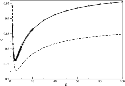
Figure 1: Pulse velocity as a function of the power of the potential. The stars represents the numerical simulation results, the continuous line the binary collision approximation, and the broken line the continuum approximation.

Herein we address the question of the applicability of both the continuum approximation and a binary interaction model through the analysis of the velocity of the signal propagation as a function of the power of the potential. For the former case, the pulse velocity, $C_{c}(n),$ can be written as ourchain

$$C_{c}(n)=\sqrt{\frac{2}{n}}\left[\frac{n^{2}(n-2)}{2(n+2)\sqrt{\frac{n(n-1)}{6}}I\left(\frac{4}{n-2}\right)}\right]^{\frac{n-2}{2n}},$$ (6)

where

$$I(l)=2^{\,l}\;\frac{\Gamma^{2}\left(\frac{l+1}{2}\right)}{\Gamma(l+1)}.$$ (7)

On the other hand, for the binary collision approximation the set of equations (5) reduces to two coupled equations which may be decoupled by defining the normal mode variables $z_{\pm}=x_{1}\pm x_{2}.$ In particular, we have

$$\ddot{z}_{-}=-2{z}_{-}^{n-1}.$$ (8)

This is precisely the equation of motion for one particle subjected to a potential $V(z)=2z^{n}/n.$ Furthermore, the initial conditions for the original variables lead to $z_{-}(0)=0$ and $\dot{z}_{-}(0)=1.$ Hence, from energy conservation we have:

$$\frac{1}{2}\dot{z}_{-}^{2}(t)-\frac{1}{2}=-\frac{2}{n}z_{-}^{n}(t).$$ (9)

Consequently, when the two particles have the same velocity ($\dot{z}_{-}=0$), their compression will be a maximum and given by $z_{m}=\left(\frac{n}{4}\right)^{1/n}$. Therefore, the time necessary for the “pulse” to travel from the first to the second particle is

$$T_{b}(n)=\int_{0}^{z_{m}}\frac{1}{\sqrt{1-4z_{-}^{n}/n}}\mathrm{d}z_{-}.$$ (10)

Explicitly integrating Eq. (10), we can write the pulse velocity $C_{b}(n)=1/T_{b}(n),$ as

$$C_{b}(n)=\frac{1}{\pi^{1/2}}\left(\frac{4}{n}\right)^{1/n}\frac{\Gamma(\frac{1}{2}+\frac{1}{n})}{\Gamma(1+\frac{1}{n})}$$ (11)

Our comparison is thus between Eqs. (6) and (11).

Figure 2: Relative error $(C_{T}-C_{S})/C_{T}$ in the pulse velocity as a function of the power of the potential. Here, the theoretical pulse velocity $C_{T}$, is either the one obtained from the continuum (circles) or from the binary collision (squares) approximation. $C_{S}$ is the pulse velocity obtained from the numerical simulations of the chain.

Qualitatively both approximations give the same result: for $n\gtrsim 2$ the pulse velocity decreases with $n$, attaining its minimum value for $n\simeq 5$, and then increasing and saturating for large $n$ (see Fig. 1). Quantitatively, however, they differ appreciably. For instance, for large $n$, $C_{b}\rightarrow 1$ while $C_{c}\rightarrow 0.883\ldots$. In Fig. 2 we present the relative error of our numerical simulation of the chain as compared with each theory. From this figure, it is easy to see that while the continuum approximation gives very good results for small $n$, its predictions are poor for $n\gtrsim 3.5$. On the other hand, the binary collision approximation is extremely accurate for $n>3.5$ but not accurate for small $n$. The quantitative agreement of each of the two analytic results at their respective $n$ extremes with the numerical simulations is seen to be excellent. Again, we stress that these results are a reflection of the behavior of the pulse width. At smaller $n$ the pulse is relatively broad, the velocity pulse covers a number of grains ourchain , and a continuum approximation captures the pulse configuration and speed very well. At larger $n$ the pulse becomes very narrow, discreteness effects dominate the behavior, and an approximation that assumes that two-grain collisions dominate the pulse behavior reproduces the pulse velocity extremely accurately.

In summary, Nesterenko’s continuum approximation gives quantitatively accurate results for the pulse velocity for relatively soft potentials, $n\lesssim 3.5$ (which includes the generic cases of cylindrical and spherical grains), while the binary collision model is quantitatively correct for relatively hard potentials, $n\gtrsim 3.5$.

References

- (1) R. S. MacKay, Phys. Lett. A 251, 191 (1999).
- (2) S. Sen and M. Manciu, Phys. Rev. E 64, 056605 (2001).
- (3) R. S. Sinkovits and S. Sen, Phys. Rev. Lett. 74, 2686 (1995).
- (4) A. Rogers and C. G. Don, Acoust. Austral. 22, 5 (1994).
- (5) C. Coste, E. Falcon, and S. Fauve, Phys. Rev. E 56, 6104 (1997).
- (6) S. Sen, M. Manciu, and J. D. Wright, Phys. Rev. E 57, 2386 (1998).
- (7) M. J. Naughton et. al., IEEE Conf. Proc. 458, 249 (1998).
- (8) E. J. Hinch and S. Saint-Jean, Proc. R. Soc. Lond. A 455, 3201 (1999).
- (9) E. Hascoët, H. J. Herrmann, and V. Loreto, Phys. Rev. E 59, 3202 (1999).
- (10) E. Hascoët and H. J. Herrmann, Eur. Phys. J. B 14, 183 (2000).
- (11) The Granular State, edited by S. Sen and M. Hunt, MRS Symp. Proc. 627 (Pittsburgh, PA, 2001).
- (12) J. Hong and A. Xu, Phys. Rev. E 63, 061310 (2001).
- (13) S. Sen et al., in Modern Challenges in Statistical Mechanics: Patterns, Noise and the Interplay of Nonlinearity and Clomplexity, edited by V. M. Kenkre and K. Lindenberg, AIP Conference Proceedings 658, 357 (2003).
- (14) D. T. Wu, Physica A 315, 194 (2002).
- (15) M. Nakagawa, J. H. Agui, D. T. Wu, and D. V. Extramiana, Granular Matter 4, 167 (2003).
- (16) E. Hascoët and E. J. Hinch, Phys. Rev. E 66, 011307 (2002).
- (17) V. F. Nesterenko, J. Appl. Mech. Tech. Phys. 5, 733 (1983).
- (18) T. R. Krishna Mohan and S. Sen, cond-mat/0304600.
- (19) A. Rosas, J. Buceta, and Katja Lindenberg, Phys. Rev. E 68, 021303 (2003).
- (20) H. Hertz, J. reine u. angew. Math. 92, 156 (1881).
- (21) L. D. Landau and E. M. Lifshitz, Theory of Elasticity (Addison- Wesley, Massachusetts, 1959), pp. 30.
- (22) A. Rosas and K. Lindenberg, to appear in Phys. Rev. E.