Coherent oscillations of current due to nuclear spins

Abstract

We propose a mechanism for very slow coherent oscillations of current and nuclear spins in a quantum dot system, that may qualitatively explain some recent experimental observations. We concentrate on an experimentally relevant double dot setup where hyperfine interaction lifts the spin blockade. We study the dependence of the magnitude and period of the oscillations on magnetic field and anisotropy.

There are significant experimental and theoretical efforts aimed to utilize and manipulate the electron spin in the context of electronic transport, those are commonly referred to as spintronicsAwshalom et al. (2002); Wolf et al. (2001). Some of them involve nuclear spins as well. Many efforts concern GaAs semiconductor structures where the hyperfine interaction between electron and nuclear spin is relatively strong Paget and Berkovits (1984). Furthermore, the nuclear spin relaxation times are much longer than the time scales related to electron dynamicsPaget et al. (1977); Paget (1982). This time scale separation has facilitated experiments where a quasi-stationary polarization of the nuclear system was achieved and its effect on the electronic transport was observed Salis et al. (2001a, b); Wald et al. (1994). Recent experiments implement novel ways of controlling the interaction of electron and nuclear spin Smet et al. (2002); Kawakami et al. (2001), whereby the coherent oscillations between ’up’ and ’down’ polarized nuclear system have been observed Machida et al. (2003).

Transport experiments with quantum dots allow for a detailed study and control of the quantum dot energy spectrum, both in the regime of linear transport and in non-linear regime of excitation spectroscopyKouwenhoven et al. (1997, 2001). They reveal interesting regimes where unusual mechanisms of electron transport are the dominant ones. For instance, in the Coulomb blockade regime the direct charging of the quantum dot is forbidden by energy conservation and the residual current is due to cotunneling Averin and Nazarov (1990); DeFranceschi et al. (2001). Another regime is the so-called spin blockade where the direct electron transfers are blocked by virtue of spin conservation Weinman et al. (1995). Spin blockade may be achieved in various ways, e. g. with spin polarized leadsCiorga et al. (2002). Recent experiment realizes the spin blockade in a double dot system, where the absence of transitions between spin-singlet and spin-triplet states in the dots explains the current rectification observed Ono et al. (2002). Any spin-flip mechanism facilitates these transitions, giving rise to a small residual current.

The same group has recently reported Ono and Tarucha an unexpected and unusual result. They have observed coherent oscillations of the residual current in this regime with a period in the range of seconds. This extremely long time scale together with the fact that the oscillation period and amplitude can be modified by resonant excitation of the nuclear spins, strongly suggests that the origin of the oscillations may be traced to the hyperfine interaction Ono and Tarucha .

In this letter we propose a concrete mechanism for these oscillations that can at least qualitatively explain the observation made in Ref. Ono and Tarucha, . The effect comes about from the dynamics of nuclear spins driven by hyperfine interaction with electron spin. The configuration of the nuclear spins can be presented with two effective magnetic fields acting on the electron spin in the two dots. The difference of these fields lifts the spin blockade thereby affecting the average current and electron spin. These fields are quasistationary at the scale of successive electron transfers. They precess around the external magnetic field ($z$-axis) with frequency $10^{7}$ Hz. Albeit this precession does not manifest itself in current oscillations. The oscillations result from slow nutations of the fields. These nutations arise from small deflection of electron spin from the $z$-axis, the deflection being induced by the fields.

The dynamics of the nuclear spin fields appears to be far from chaotic so that the period and magnitude of the oscillations strongly depend on initial conditions of the nuclear spin system. Therefore the comparison with experiment may be only qualitative. In reality, the relaxation of nuclear spin would lead to stabilization of the oscillations with a certain amplitude and period. However, such stabilizing mechanisms would manifest itself at time scale much longer than the period. This is why we do not consider them in the present model.

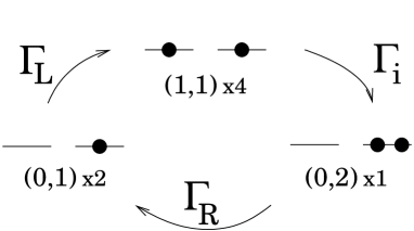
Figure 1: Each charge configuration is characterized by ($N_{L}$,$N_{R}$) and also its multiplicity. The three charge transfer processes are ($i$) electron entering the left dot from the left lead, ($ii$) electron going from left dot to right dot, and ($iii$) electron leaving the right dot to the right lead. See text for discussion on the $\Gamma$’s.

For details of the setup we refer the reader to Ref. Ono et al., 2002. In the regime of interest, the double dot can be in three distinct charge configurations as shown in Fig. 1. A charge configuration is characterized by ($N_{L}$,$N_{R}$), $N_{L}$($N_{R}$) being the number of electrons in the left (right) dot. Transitions from (0,1) to (1,1) and from (0,2) to (0,1) are relatively fast involving electron tunneling either from the left or to the right lead with the rates $\Gamma_{L,R}$. The bottleneck of the transport cycle are transitions between (1,1) and (0,2). In the (0,2) configuration both electrons share the same orbital state, this makes it a non-degenerate spin singlet. In contrast to this, the (1,1) configuration comprises 4 possible states, grouped into spin-singlet and spin-triplet. The transitions between the (1,1) singlet and (0,2) occur with the rate $\Gamma_{i}$ that is determined by the tunneling amplitude between the dots and a relevant mechanism of inelastic scattering, e.g. phonons. These transitions do not require any spin-flip. The transitions between the (1,1) triplet states and (0,2) singlet are forbidden by spin conservation: this causes the spin blockade.

The hyperfine interaction with nuclei induces mixing of the singlet and triplet states in the $(1,1)$ configuration. The part of the total Hamiltonian which contains the electron and nuclear spin operators reads

$$H_{s}=\hat{\bm{K}_{L}}\cdot\hat{\bm{S}}_{L}+\bm{K}_{R}\cdot\hat{\bm{S}}_{R}+E_{Z}\cdot(\hat{S}^{z}_{L}+\hat{S}^{z}_{R})+$$

$$\Delta_{ST}(\hat{\bm{S}}_{L}+\hat{\bm{S}}_{R})^{2}/2.$$ (1)

Here $\hat{\bm{S}}_{L,R}$ are operators of electron spin in each dot . The effect of nuclear spins is combined into two effective fields $\hat{\bm{K}}_{L,R}$. In each dot

$$\hat{\bm{K}}_{L,R}=\hbar\sum_{k}\gamma_{L,R;k}\hat{\bm{I}}_{k};\;\;\gamma_{L,R;k}=\hbar^{-1}A|\psi_{L,R}(\bm{R}_{k})|^{2}$$ (2)

where $\hat{\bm{I}}_{k}$ being operators of nuclear spin at $\bm{R}_{k}$, the summation goes over all nuclei and precession frequencies $\gamma_{k}$ are set by an envelop of electron wave function and hyperfine constant $A$. The third term in Eq. 1 represents the Zeeman splitting $E_{Z}$ in the external magnetic field while the fourth term represents the exchange splitting between the singlet and triplet. We adopt a semiclassical approximation of the effective fields $\bm{K}_{L,R}$ replacing them by classical variablesD’yakonov and Kachorovksii (1986); Merkulov et al. (2002); Erlingsson and Nazarov (2002). This approximation is justified by a big number of nuclei in the dots, $N_{\mbox{\scriptsize QD}}\gg 1$. The third and fourth terms in Eq. (1) include the full spin only and therefore split the states onto singlet and three Zeeman-split triplet components. The mixing of these states is proportional to the difference of two effective fields $\bm{K}_{A}\equiv\bm{K}_{L}-\bm{K}_{R}$.

The mixing thus lifts spin blockade. We assume that this mixing is the only mechanism of the residual current. This assumption is not crucial since alternative mechanisms, those include co-tunneling and non-nuclear spin-flips, would only produce an extra d.c. current background for nuclear-induced current oscillations.

We solve the problem in two steps. First, we solve for the density matrix of electron states assuming stationary $\bm{K}_{L,R}$. The output of the calculation are the average current and the average electron spin $\langle\bm{S}_{L,R}\rangle$ in terms of $\bm{K}_{L,R}$. Second, we use this output to derive equations for the dynamics of $\bm{K}_{L,R}$ and subsequently analyze this dynamics. This approach relies on the time scale separation: the fields $\bm{K}_{L,R}$ should not change at the time scale of successive electron transfers. The transfer rate can be estimated as ($E_{Z}\simeq\Delta_{ST}$) $(K_{A}/\Delta_{ST})^{2}\Gamma_{i}$. The small factor $(K_{A}/\Delta_{ST})$ is the ratio of the mixing and energy difference between singlet and triplet states and quantifies suppression of the current in the spin blockade regime. The fastest nuclear spin motion that changes $\bm{K}$ is the precession around external magnetic field with frequency $\omega_{NMR}\simeq 10^{7}$ Hz. This results in the condition $\Gamma_{i}\gg(\Delta_{ST}/K_{A})^{2}\omega_{NMR}$ for the validity of our approach. As we see below, the current oscillations are much slower with a typical period of the order of $\gamma^{-1}(\Delta_{ST}/K_{A})$, where $\gamma=(\gamma_{L}+\gamma_{R})/2$. The precession frequency and typical magnitude of effective field can be estimated Erlingsson and Nazarov (2002) as $\gamma\simeq E_{n}/N_{QD}$, $K\simeq E_{n}/\sqrt{N_{QD}}$, where $E_{n}\approx 0.135$ meV in GaAs and $N_{\mbox{\scriptsize QD}}\approx$10⁶ for the quantum dots in question. The exchange splitting $\Delta_{ST}\propto 10^{-5}-10^{-4}eV$ as estimated in Ref. Ono and Tarucha, . This gives $\gamma^{-1}(\Delta_{ST}/K_{A})\simeq 0.01-0.1$ sec.

To make the first step, we describe the evolution of the electron system with Bloch equations for the density matrix approach. There are seven quantum states involved in the transport ($|s\rangle$ for the singlet in the (0,2) configuration, $|+\rangle$ and $|-\rangle$ for the two doublet components in the (1,0) configuration ,$|0\rangle$ for the singlet and $|1\rangle,|2\rangle,|3\rangle$ for triplet states in the (1,1) configuration, those correspond to $S_{z}=1,0,-1$ respectively) so that the full density matrix comprises of $49$ elements. However, we can disregard most of the non-diagonal elements of the matrix except those between 4 states of the (1,1) configuration. So we end up with 19 equations only. We present here 3, this suffices to illustrate the overall structure.

$$\frac{d\rho_{11}}{dt} = \frac{\Gamma_{L}}{2}\rho_{++}+\Im\{K^{+}_{A}\rho_{10}\}$$ (3a)

$$\frac{d\rho_{00}}{dt} = -\Gamma_{i}\rho_{00}+\frac{\Gamma_{L}}{4}\bigl{(}\rho_{++}+\rho_{--}\bigr{)}$$ (3b)

$$+\Im\{-K_{A}^{+}\rho_{10}+K_{A}^{z}\rho_{20}+K_{A}^{-}\rho_{30}\}$$

$$\frac{d\rho_{10}}{dt} = -i\bigl{(}\Delta_{ST}+E_{Z})+i\frac{\Gamma_{i}}{2}\bigr{)}\rho_{10}+\frac{1}{2}\bigl{(}-iK_{A}^{-}(\rho_{11}\!\!-\!\!\rho_{00})$$ (3c)

$$+iK_{A}^{z}\rho_{12}+iK_{A}^{+}\rho_{13}\bigr{)},$$

where $K_{A}^{\pm}=(K_{A}^{x}\pm iK_{A}^{y})/\sqrt{2}$. Note that the inelastic rate $\Gamma_{i}$ does not appear in Eq. (3a), the same is true for the other triplets, but it is present in Eq. (3b) for the singlet. The average electron spins in each dot and the current can be readily obtained from the stationary solution $\hat{\rho}^{\mbox{\scriptsize\,st}}$ of Eq. (3): $\langle{\bm{S}}_{L,R}\rangle=\mbox{Tr}\{\hat{\rho}^{\mbox{\scriptsize\,st}}\hat{\bm{S}}_{L/R}\}$, $I=e\Gamma_{R}\rho^{\mbox{\scriptsize\,st}}_{ss}$. We do not need to present the cumbersome full solutions for the average spin here. Instead, we assume $\Gamma_{in}\ll\Gamma_{L,R},\Delta_{ST}/\hbar$ and note that in the zeroth order in $K_{A}/\Delta_{ST}$ the average spin is in the $z$-direction and ($x_{B}\equiv E_{Z}/\Delta_{ST}$)

$$\langle S^{z}_{L,R}\rangle=-\frac{2E_{Z}}{\Delta_{ST}}S;\;\;S^{-1}\equiv 2(1+x^{2}_{B})+\left(\frac{|K_{A}^{+}|}{K_{Az}}\right)^{2}.$$ (4)

With the same accuracy the current reads

$$\frac{I}{e}=\left(\frac{|K_{A}^{+}|}{\Delta_{ST}}\right)^{2}4S\Gamma_{i}.$$ (5)

In addition, we need the deflections of $\langle\bm{S}_{L,R}\rangle$ from the $z$-direction. They arise in the next order in $K_{A}/\Delta_{ST}$ and are antiparallel in opposite dots:

$$\left(\begin{array}[]{ccc}\langle S^{x}_{L,R}\rangle\cr\langle S^{y}_{L,R}\rangle\cr\langle S^{z}_{L,R}\rangle\end{array}\right)=\pm\frac{S}{2\Delta_{ST}}\left(\begin{array}[]{ccc}K^{x}_{A}\cr K^{y}_{A}\cr\frac{|K^{+}_{A}|^{2}}{K^{z}_{A}}\end{array}\right).$$ (6)

Now we perform the second step and describe the dynamics of the effective fields. To simplify, we will assume the same electron precession frequencies for all nuclei in each dot: $\gamma_{L,R;k}=\gamma_{L,R}$. The advantage of this model is a closed system of equations for the collective fields:

$$\frac{d}{dt}\bm{K}_{\alpha}=\gamma_{\alpha}\langle\bm{S}_{\alpha}\rangle\times\bm{K}_{\alpha}+\gamma_{\mbox{\scriptsize GaAs}}\bm{B}\times\bm{K}_{\alpha}$$ (7)

($\alpha=L,R$) that describes precession of these fields, their moduli $K_{L,R}$ being constants of motion. The main precession is around external magnetic field with the frequency $\gamma_{\mbox{\scriptsize GaAs}}|B|$. However, this precession is irrelevant since it does not change the $K^{z}_{L,R}$ and the angle $\phi$ between the projections of these vectors onto $xy$ plane. These three slow variables actually determine the average spin and current, and the evolution equations for those

$$\frac{d}{dt}K^{z}_{\alpha} = \gamma_{\alpha}(\langle S^{x}_{\alpha}\rangle K^{x}_{\alpha}-\langle S^{y}_{\alpha}\rangle K^{y}_{\alpha})$$

$$\frac{d}{dt}\phi = \gamma_{L}\langle S^{z}_{L}\rangle-\gamma_{R}\langle S^{z}_{R}\rangle,$$ (8)

do not contain $\gamma_{\mbox{\scriptsize GaAs}}B\gg\gamma_{L,R}\langle S_{L,R}\rangle$. These three equations have an extra integral of motion, $K^{z}_{S}\equiv(K^{z}_{L}\gamma_{R}+K^{z}_{R}\gamma_{L})/2\gamma$. Moreover, the equation for two remaining variables appears to be of a Hamiltonian type. In dimensionless variables $k\equiv K^{z}_{A}/K_{L},\tau=t\gamma K_{L}/\Delta_{ST}$ the equations read

$$\frac{d}{d\tau}\left(\begin{array}[]{cc}k\cr\phi\end{array}\right)=\frac{k^{2}}{(b-\cos\phi)Y}\left(\begin{array}[]{rr}\frac{\partial}{\partial\phi}\cr-\frac{\partial}{\partial k}\end{array}\right){\cal L}$$ (9)

where

$$\mathcal{L}(k,\phi) = X(k)+Y(k)\cos\phi,$$

$$X(k) = -\frac{1+k_{R}^{2}-2(k^{z}_{S})^{2}}{2}k+2\epsilon x_{B}k^{2}+\frac{k^{3}}{4},$$

$$Y(k) = k\sqrt{(1-(k^{z}_{S}+k/2)^{2})(k_{R}^{2}-(k^{z}_{S}-k/2)^{2})},$$

$$b(k) = \frac{(\frac{7}{4}+2x_{B}^{2})k^{3}+\frac{k}{2}(1+k_{R}^{2}-2(k^{z}_{S})^{2})}{Y(k)},$$ (10)

and we introduced the notations $k_{R},k^{z}_{S}\equiv K_{R}/K_{L},K^{z}_{S}/K_{L}$ and $\epsilon=(\gamma_{L}-\gamma_{R})\Delta_{ST}/2\gamma K_{L}$. We also assume here that the asymmetry of electron precession frequencies is small, $\delta\gamma\equiv|\gamma_{L}-\gamma_{R}|\ll\gamma_{L,R}$. One would expect this for the experiment in question since the two dots are nominally identical

The $\cal{L}$ is evidently yet another constant of motion that depend on initial condition of the nuclear system. The solution of $\mathcal{L}=L$, if it exists, determines a closed orbit in the $(k,\phi)$ phase space and the system experiences periodic motion along this orbit. This motion manifests itself in the current oscillations by virtue of Eq. 5. The period and magnitude of the oscillations do depend on the initial conditions $L,k_{R},k^{z}_{S}$. If $L$ is close to $0$, the period even diverges. There is, however, some regular dependence on the asymmetry $\epsilon$ and the external magnetic field that enters through parameter $x_{B}$, see Fig. 2. This dependence can be summarized as follows. The period $T$ depends on asymmetry. If $\epsilon x_{B}\lesssim 1$, $T\simeq\gamma^{-1}\Delta_{ST}/K_{L}$ for $x_{B}\lesssim 1$ and $T\simeq\gamma^{-1}E^{2}_{Z}/\Delta_{ST}K_{L}$ for $x_{B}\gg 1$. In the opposite case of relatively large asymmetry $\epsilon x_{B}\gg 1$, $T\simeq(x_{B}\delta\gamma)^{-1}$ for $x_{B}\ll 1$ and $T\simeq x_{B}(\delta\gamma)^{-1}$ for $x_{B}\gg 1$. Also, the amplitude of the oscillations relative to the average current is of the order of $1$ for $x_{B}\lesssim 1$ and decreases as $x^{-2}_{B}$ for $x_{B}\gg 1$.

The initial values of $\bm{K}_{\alpha}$ that determine the actual magnitude and period of the oscillations are distributed according to Gaussian statistics Erlingsson and Nazarov (2002) with average squares corresponding to average squares of total nuclear spins in the dot. In Fig. 3 the current, see Eq. (5), is plotted for various initial conditions but fixed $\epsilon=0.1$ and $x_{B}=1.6$. We note apparent anharmonicity of the oscillations, this feature has been stressed in Ref. Ono and Tarucha, .

One might think that the periodic oscillations we obtained in our approach is an artefact of oversimplified model for nuclear dymanics in use. Recent work emphasizes the importance of the fact that precession frequency $\gamma_{k}$ varies from nucleus to nucleus Khaetskii et al. (2002). This issue can be addressed within the semiclassical approach used here. To implement such approach numerically, we separate the nuclear spin system into $N_{b}\gg 1$ blocks where the $\gamma_{k}$’s are the same within each block but differ from block to block. The number of spins remains large so that the nuclear dynamics can be described in terms of effective fields $\bm{K}^{(b)}_{L,R}$. This results in $6N_{b}$ evolution equations similar to Eqs. 8. Intuitively, one expects such complicated dynamics to be chaotic, so that the memory about initial conditions is lost after some time $\simeq\gamma^{-1}$. This would be really dreadful for the mechanism discussed, so we have performed extensive numerical simulations to check this circumstance Erlingsson and Nazarov . To summarize the results, the dynamics is not chaotic, the memory about initial conditions persists and the nuclear system exhibits regular oscillations, typically with several periods. To illustrate this fact, we present a typical result in the inset of Fig. 3. It shows the regular long-period motion and extra fast oscillations on the timescale of $\gamma^{-1}$.

In conclusion, we propose a mechanism whereby the transport via a double quantum dot induces slow regular nutations of the nuclear spin system, these nutations are seen in the transport current. We model the concrete experimental situation (Ono and Tarucha ) and our estimations of the typical frequency, anharmonic shape of the oscillation predicted, and sensitivity to magnetic field shown correspond to the observations made in Ono and Tarucha . More research on relevant nuclear spin relaxation mechanisms is needed for detailed comparison with the experiment. From the other hand, the mechanism presented is sufficiently general and works in any conditions where the hyperfine interaction provides the main mechanism of spin blockade lifting.

We are grateful to the authors of Ref. Ono and Tarucha for communicating their results prior to publication. We acknowledge the financial support by FOM.

Figure 2: The period as a function the integral of motion $L$ for various values of $x_{B}$. The asymmetry is $\epsilon=0.1$, $k_{R}=0.9$ and $k_{S}^{z}=0.0$. The inset shows the period as a function of $x_{B}$ for fixed values of $L$.

Figure 3: The current shown as a function of time for $\epsilon$=0.1, $x_{B}$=1.6, but for different initial conditions, i.e. different $L$. The inset shows current for $L=-0.14$ in the case of $N_{b}$=1 and 25, where $N_{b}$ is the number of blocks. Note that the long period oscillations are still present for $N_{b}\gg 1$.

References

- Awshalom et al. (2002) D. D. Awshalom, D. Loss, and N. Samarth, eds., Semiconductor Spintronics and Quantum Computation (Springer-Verlag, Berlin, 2002).
- Wolf et al. (2001) S. A. Wolf, D. D. Awschalom, R. A. Buhrman, J. M. Daughton, S. von Molnár, M. L. Roukes, A. Y. Chtchelkanova, and D. M. Treger, Science 294, 1488 (2001).
- Paget and Berkovits (1984) D. Paget and V. L. Berkovits, Optical Orientation (North-Holland, Amsterdam, 1984).
- Paget et al. (1977) D. Paget, G. Lampel, B. Sapoval, and V. I. Safarov, Phys. Rev. B 15, 5780 (1977).
- Paget (1982) D. Paget, Phys. Rev. B 25, 4444 (1982).
- Salis et al. (2001a) G. Salis, D. T. Fuchs, J. M. Kikkawa, D. Awschalom, Y. Ohno, and H. Ohno, Phys. Rev. Lett. 86, 2677 (2001a).
- Salis et al. (2001b) G. Salis, D. D. Awschalom, Y. Ohno, and H. Ohno, Phys. Rev. B 64, 195304 (2001b).
- Wald et al. (1994) K. R. Wald, L. P. Kouwenhoven, P. L. McEuen, N. C. van der Vaart, and C. T. Foxon, Phys. Rev. Lett. 73, 1011 (1994).
- Smet et al. (2002) J. H. Smet, R. A. Deutchmann, F. Ertl, W. Wegscheider, G. Abstreiter, and K. von Klitzing, Nature 415, 281 (2002).
- Kawakami et al. (2001) R. K. Kawakami, Y. Kato, M. Hanson, I. Malajovich, J. M. Stephens, E. Johnston-Halperin, G. Salis, A. C. Gossard, and D. D. Awschalom, Science 294, 131 (2001).
- Machida et al. (2003) T. Machida, T. Yamazaki, K. Ikushima, and S. Komiyama, App. Phys. Lett. 82, 409 (2003).
- Kouwenhoven et al. (1997) L. P. Kouwenhoven, C. M. Marcus, P. L. McEuen, S. Tarucha, R. M. Westervelt, and N. S. Windgreen, Mesoscopic Electron Transport (Kluwer, Dordrecht, 1997), chap. Electron transport in quantum dots, p. 105, NATO Series.
- Kouwenhoven et al. (2001) L. P. Kouwenhoven, D. G. Austing, and S. Tarucha, Rep. Prog. Phys. 64, 701 (2001).
- Averin and Nazarov (1990) D. V. Averin and Y. V. Nazarov, Phys. Rev. Lett. 65, 2446 (1990).
- DeFranceschi et al. (2001) S. DeFranceschi, S. Sasaki, J. M. Elzerman, W. G. van der Wiel, S. Tarucha, and L. P. Kouwenhoven, Phys. Rev. Lett. 86, 878 (2001).
- Weinman et al. (1995) D. Weinman, W. Häussler, and B. Kramer, Phys. Rev. Lett. 74, 984 (1995).
- Ciorga et al. (2002) M. Ciorga, M. Pioro-Ladriere, P. Zawadzki, P. Hawrylak, and A. S. Sachrajda, App. Phys. Lett. 80, 2177 (2002).
- Ono et al. (2002) K. Ono, D. G. Austing, Y. Tokura, and S. Tarucha, Science 297, 1313 (2002).
- (19) K. Ono and S. Tarucha, (unpublished).
- D’yakonov and Kachorovksii (1986) M. I. D’yakonov and V. Y. Kachorovksii, Sov. Phys. Semicond. 20, 110 (1986).
- Merkulov et al. (2002) I. A. Merkulov, A. L. Efros, and M. Rosen, Phys. Rev. B 65, 205309 (2002).
- Erlingsson and Nazarov (2002) S. I. Erlingsson and Y. V. Nazarov, Phys. Rev. B 66, 155327 (2002).
- Khaetskii et al. (2002) A. V. Khaetskii, D. Loss, and L. Glazman, Phys. Rev. Lett. 88, 186802 (2002).
- (24) S. I. Erlingsson and Y. V. Nazarov, (in preparation).