Finite size effect in Bi₂Sr₂CaCu₂O_8+δ and YBa₂Cu₃O_6.7 probed by the in-plane and out of plane penetration depths

Abstract

We report on a systematic finite size scaling analysis of in-plane penetration depth data taken on Bi₂Sr₂CaCu₂O_8+δ epitaxially-grown films and single crystals, and of in-plane and out of plane data taken on YBa₂Cu₃O_6.7 aligned powder. It is shown that the tails in temperature dependence of the penetration depths, appearing around the transition temperature, are fully consistent with a finite size effect. This uncovers the granular nature of these cuprates, consisting of superconducting homogeneous domains of nanoscale extent, embedded in a non-superconducting matrix.

Since the discovery of superconductivity in cuprates by Bednorz and Müller[1] a tremendous amount of work has been devoted to their characterization. The issue of inhomogeneity and its characterization is essential for several reasons, including: First, if inhomogeneity is an intrinsic property, a re-interpretation of experiments, measuring an average of the electronic properties, is unavoidable. Second, inhomogeneity may point to a microscopic phase separation, i.e. superconducting grains, embedded in a non superconducting matrix. Third, there is neutron spectroscopic evidence for nanoscale cluster formation and percolative superconductivity in various cuprates[2, 3]. Fourth, nanoscale spatial variations in the electronic characteristics have been observed in underdoped Bi₂Sr₂CaCu₂O_8+δ with scanning tunnelling microscopy (STM)[4, 5, 6, 7]. They reveal a spatial segregation of the electronic structure into 3nm diameter superconducting domains in an electronically distinct background. On the contrary, a large degree of homogeneity has been observed by Renner and Fischer[8]. As STM is a surface probe, the relevance of these observations for bulk and thermodynamic properties has been clarified in terms of a finite size scaling of specific heat and London penetration depth data, revealing $\ L_{ab}\approx 50\AA$ and $L_{c}\approx 68\AA$ for the length scale of the superconducting domains along the c-axis and in the ab-plane, respectively [9]. Fifth, superconducting domains with $\ L_{ab}\approx 300\AA$ were revealed by x-ray diffraction in oxygen doped La₂CuO₄ single crystal [10]. Sixth, in YBa₂Cu₃O_7-δ, MgB₂, 2H-NbSe₂ and Nb₇₇Zr₂₃ considerably larger domains have been established. The magnetic field induced finite size effect revealed lower bounds ranging from $L=182$ to $814$Å[11].

This paper addresses these issues by performing a detailed finite size scaling analysis of the tails in the measured temperature dependence of the penetration depths, appearing around the transition temperature. Specifically we analyze the data taken on Bi₂Sr₂CaCu₂O_8+δ in the form of epitaxially-grown films[12] and high quality single crystals[13, 14], and on magnetically aligned YBa₂Cu₃O_6.7 powder[15]. The paper is organized as follows. Next we sketch the finite size scaling theory adapted for the analysis of penetration depth data. Then we analyze the experimental data and establish the consistency with a finite size effect, uncovering the granular nature of these cuprates, consisting of homogeneous superconducting domains with nanoscale extent, embedded in a non-superconducting matrix.

Supposing that cuprate superconductors are granular, consisting of spatial superconducting domains, embedded in a non-superconducting matrix and with spatial extent $L_{a}$, $L_{b}$ and $L_{c}$ along the crystallographic a, b and c-axis. in this case the correlation length $\xi_{i}$ in direction $i$, increasing strongly when $T_{c}$ is approached cannot grow beyond $L_{i}$. Consequently, for finite superconducting domains, the thermodynamic quantities, like the specific heat and penetration depth, are smooth functions of temperature. As a remnant of the singularity at $T_{c}$ these quantities exhibit a so called finite size effect[16], namely a maximum or an inflection point at $T_{p_{i}}$, where $\xi_{i}\left(T_{p_{i}}\right)=L_{i}$. There is mounting experimental evidence that, for the accessible temperature ranges, the effective finite temperature critical behavior of the cuprates is controlled by the critical point of uncharged superfluids (3D-XY)[12, 17]. In this case there is the universal relationship

$$\frac{1}{\lambda_{i}^{2}\left(T\right)}=\frac{16\pi^{3}k_{B}T}{\Phi_{0}^{2}\xi_{i}^{t}\left(T\right)},$$ (1)

between the London penetration depth $\lambda_{i}$ and the transverse correlation length $\xi_{i}^{t}$ in direction $i$[17]. As aforementioned, when the superconductor is inhomogeneous, consisting of superconducting grains with length scales $L_{i}$, embedded in a non-superconducting matrix, the $\xi_{i}^{t}$’s do not diverge but are bounded by

$$\xi_{i}^{t}\xi_{j}^{t}\leq L_{k}^{2},\ i\neq j\neq k.$$ (2)

A characteristic feature of the resulting finite size effect is the occurrence of an inflection point at $T_{p_{k}}$ below $T_{c}$, the transition temperature of the homogeneous system. Here

$$\xi_{i}^{t}\left(T_{p_{k}}\right)\xi_{j}^{t}\left(T_{p_{k}}\right)=L_{k}^{2},\ i\neq j\neq k,$$ (3)

and Eq.(1) reduces to

$$\left.\frac{1}{\lambda_{i}\left(T\right)\lambda_{j}\left(T\right)}\right|_{T=T_{p_{k}}}=\frac{16\pi^{3}k_{B}T_{p_{k}}}{\Phi_{0}^{2}}\frac{1}{L_{k}}.$$ (4)

In the homogeneous case $1/\left(\lambda_{i}\left(T\right)\lambda_{j}\left(T\right)\right)$ decreases continuously with increasing temperature and vanishes at $T_{c}$, while for superconducting domains, embedded in a non-superconducting matrix, it does not vanish and exhibits a turning point at $T_{p_{k}}<T_{c}$, so that

$$\left.d\left(\frac{1}{\lambda_{i}\left(T\right)\lambda_{j}\left(T\right)}\right)/dT\right|_{T=T_{p_{k}}}=0$$ (5)

Since the experimental data for the temperature dependence of the penetration depths is available in the form $\lambda_{ab}$ and $\lambda_{c}$ only, we rewrite Eq.(4) as

$$L_{c}=\frac{16\pi^{3}k_{B}T_{p_{c}}\left(\lambda_{a}\left(T\right)\lambda_{b}\left(T\right)\right)_{T=T_{p_{c}}}}{\Phi_{0}^{2}}\approx\frac{16\pi^{3}k_{B}T_{p_{c}}\lambda_{ab}^{2}\left(T_{p_{c}}\right)}{\Phi_{0}^{2}},$$ (6)

and

$$L_{b}=\frac{16\pi^{3}k_{B}T_{p_{b}}\left(\lambda_{a}\left(T\right)\lambda_{c}\left(T\right)\right)_{T=T_{p_{b}}}}{\Phi_{0}^{2}}\approx L_{ab}=\frac{16\pi^{3}k_{B}T_{p_{b}}\left(\lambda_{ab}\left(T\right)\lambda_{c}\left(T\right)\right)_{T=T_{p_{ab}}}}{\Phi_{0}^{2}}$$ (7)

to derive estimates for the diameter of the superconducting grains along the c-axis and parallel to the ab-plane. Noting that in the homogeneous system the transverse correlation lengths diverge as

$$\xi_{i}^{t}\left(T\right)=\xi_{0i}^{t}\left|t\right|^{-\nu},\ t=\frac{T}{T_{c}}-1,\ \nu\approx 2/3,$$ (8)

the critical amplitudes and associated critical properties of the homogeneous system can also be derived from a finite size analysis. From Eqs.(6) and (7) we obtain the relations

$$\xi_{ab}^{t}\left(T_{p_{c}}\right)=L_{c},\ \sqrt{\xi_{ab}^{t}\left(T_{p_{ab}}\right)\xi_{c}^{t}\left(T_{p_{ab}}\right)}=L_{ab}.$$ (9)

Indeed, the transverse correlation lengths cannot grow beyond the corresponding limiting length scales. Thus given $T_{p_{c}}$and $L_{c}$, $T_{p_{ab}}$ and $L_{ab}$, the critical amplitudes $\xi_{0ab}^{t}$ and $\xi_{0c}^{t}$ are readily derived. The anisotropy follows then from

$$\gamma=\left(\frac{\xi_{0c}^{t}}{\xi_{0ab}^{t}}\right)^{1/2}=\frac{\lambda_{0c}}{\lambda_{0ab}}.$$ (10)

As the system feels its finite size when the correlation length becomes of the order of the confining length, a physical quantity $O$ adopts the scaling form[18]

$$\frac{O\left(t,L\right)}{O\left(t,L=\infty\right)}=f\left(x\right),\ x=\frac{L}{\xi\left(t,L=\infty\right)}.$$ (11)

The point is that the scaling function $f$ depends only on the dimensionless ratio $L/\xi\left(t,L=\infty\right)$ and it does not depend on microscopic details of the system. It does, however, depend on the observable $O$, the type of confining geometry and on the conditions imposed (or not, in the case of free boundaries) at the boundaries of the domains. Considering the London penetration depth, it reduces to

$$\frac{\lambda_{0i}\lambda_{0j}}{\lambda_{i}\lambda_{j}}\left|t\right|^{-\nu}=f\left(\frac{sign\left(t\right)L_{k}\left|t\right|^{\nu}}{\sqrt{\xi_{0i}^{t}\xi_{0j}^{t}}}\right)=g\left(y\right),\ \ y=sign\left(t\right)\left|t\right|\left(\frac{L_{k}}{\sqrt{\xi_{0i}^{t}\xi_{0j}^{t}}}\right)^{1/\nu}=sign\left(t\right)\left|\frac{t}{t_{p_{k}}}\right|$$ (12)

For $t$ small and $L_{k}\rightarrow\infty$, $\pm y\rightarrow\infty$ and

$$g\left(y\rightarrow-\infty\right)=1,\ g\left(y\rightarrow\infty\right)=0$$ (13)

while for $t=0$ and $L_{k}\neq 0$

$$g\left(y\rightarrow 0\right)=g_{0k}y^{-\nu}=g_{0k}\left(\left|\frac{t}{t_{p_{k}}}\right|\right)^{-\nu},$$ (14)

so that in this limit

$$\frac{\lambda_{0i}\lambda_{0j}}{\lambda_{i}\left(T_{c},L_{k}\right)\lambda_{j}\left(T_{c},L_{k}\right)}=g_{0k}\frac{\sqrt{\xi_{0i}^{t}\xi_{0j}^{t}}}{L_{k}}.$$ (15)

As expected, a sharp superconductor to normal state transition requires domains of infinite extent. Moreover at $t_{p}$, $y=1$ and $d\left(\lambda_{0i}\lambda_{0j}/\left(\lambda_{i}\left(T\right)\lambda_{j}\left(T\right)\right)\right)/dt=0$. Accordingly, there is an inflection point at $T_{p_{k}}$. Since the scaling function $g\left(y\right)$ depends on the type of confining geometry and on the conditions imposed (or not, in the case of free boundaries) at the boundaries of the domains, this applies to the amplitude $g_{0k}$ as well.

We are now prepared to analyze the extended and systematic penetration depth data of Osborn  et al.[12] derived from complex conductivity measurements on epitaxially-grown Bi₂Sr₂CaCu₂O_8+δ films using a two-coil inductive technique at zero applied field. In Fig.1 we displayed the temperature dependence of the real part of the complex superfluid density which is proportional to $1/\lambda_{ab}^{2}$ for films A, B and C with different doping level. For comparison we included the leading critical behavior in terms of

$$Re\left(\rho\right)=Re\left(\rho\right)_{0}\left|t\right|^{\nu},\ \nu\simeq 2/3$$ (16)

with the parameters listed in Table I. Apparently the data is inconsistent with such a sharp transition. It clearly uncovers a rounded transition which occurs smoothly and with that a finite size effect at work. Indeed the extreme in $d\Re\left(\rho\right)/dT$ clearly reveals the existence of an inflection point at $T_{p}$ below the bulk $T_{c}$, where the transverse correlation length $\xi_{ab}^{t}$ attains the limiting length along the c-axis (Eq.(9)). Using the estimates for $T_{p}$, derived from the location of the extremum in $d\Re\left(\rho\right)/dT$ values for $L_{c}$ are now readily calculated with the aid of Eq.(6) and the parameters listed in Table I. The results included in this table clearly point to the nanoscale nature of the inhomogeneities along the c-axis. Nevertheless, due to the small critical amplitude of the transverse correlation length $\xi_{0ab}^{t}$, which follows from Eq.(3) and the corresponding parameters listed in Table I, and the fact that $L_{c}$ is considerably smaller than the film thickness $d$, the critical 3D-XY critical regime is attained.

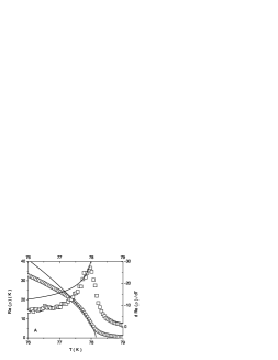
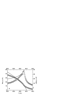
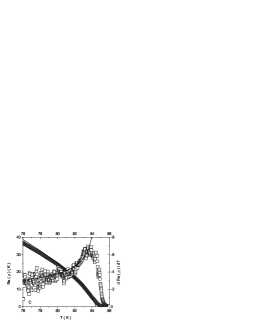
FIG. 1.: $Re\left(\rho\right)\propto 1/\lambda_{ab}^{2}$ and $dRe\left(\rho\right)/dT$ versus $T$ for films A, B and C taken from Osborn  et al.[12]. The solid lines indicate the leading critical behavior of a homogeneous bulk system according to Eq.(16) with the parameters listed in Table I.

	A	B	C	SC1	SC1	SC2
$T_{c}$ (K)	78.15	84	84.4	87.5	87.5	91
$T_{p_{c}}$ (K)	77.97	83.77	83.73	87	87	90.5
$-t_{p_{c}}$	0.0023	0.0027	0.0079	0.0057	0.0057	0.0055
$Re\left(\rho\right)_{0}$ ( K )	450	650	180	-	-
$\left(\lambda_{ab}\left(0\right)/\lambda_{0ab}\right)^{2}$	-	-	-	1.25	1.25	1.65
$\lambda_{ab}\left(0\right)$ (nm)	235	265	285	180	250	185
$Re\left(\rho\left(0\right)\right)$ ( K )	169.3	135.1	116.9	-	-
$Re\left(\rho\left(T_{p_{c}}\right)\right)$ ( K )	8.51	13.66	7.1	-	-
$\left(\lambda_{ab}\left(0\right)/\lambda_{ab}\left(T_{p_{c}}\right)\right)^{2}$	-	-	-	0.066	0.066	0.062
$L_{c}$ (Å)	137	93	180	68	132	80
$\xi_{0ab}^{t}$ (A)	2.39	1.8	7.14	2.17	4.21	2.5
$d$ ( Å)	323	616	924	-	-
$\left(\lambda_{0ab}\left(0\right)/\lambda_{ab}\left(T_{c}\right)\right)^{2}$	-	-	-	0.045	0.045	0.038
$Re\left(\rho\left(T_{c}\right)\right)/Re\left(\rho\right)_{0}$	0.097	0.011	0.018	-	-
g0	0.6	0.6	0.6	1.6	1.6	1.2
$g_{0}\xi_{0ab}^{t}/L_{c}$	0.010	0.011	0.024	0.051	0.051	0.038

Table I: Estimates entering and resulting from the finite size scaling analysis of the in-plane penetration depth data of Bi₂Sr₂CaCu₂O_8+δ films (A,B,C) and single crystals (SC1 and SC2). The films are respectively, A overdoped, B slightly overdoped and C underdoped.

To extend the analysis further we consider the finite size scaling function entering Eq.(12) in terms of

$$g\left(\frac{t}{\left|t_{p_{c}}\right|}\right)=\left|t\right|^{-\nu}\frac{Re\left(\rho\right)}{Re\left(\rho\right)_{0}}.$$ (17)

In Fig.2 we displayed this finite size scaling function for films A, B and C. The collapse of the data on a single curve indicates that the inhomogeneities, also differing in their extent $L_{c}$, have nearly the same shape and are subject to the same boundary conditions. Indeed close to $t=0$ the data approaches the expected behavior (Eq.(12))

$$g\left(\frac{t}{\left|t_{p_{c}}\right|}\right)=g_{0c}\left|\frac{t}{t_{p_{c}}}\right|^{-2/3},$$ (18)

and $g_{0c}\simeq 0.6$. Moreover rewriting Eq.(15) in the form

$$\frac{Re\left(\rho\left(T_{c}\right)\right)}{Re\left(\rho\right)_{0}}=g_{0c}\left|t_{p_{c}}\right|^{\nu}=\frac{g_{0c}\xi_{0ab}^{t}}{L_{c}},$$ (19)

this relation provides a consistency test of the estimates for $g_{0c}$, $\xi_{0ab}^{t}$ and $L_{c}$. From Table I it is seen that there is satisfactory agreement.

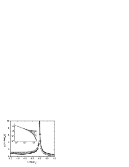
FIG. 2.: Finite size scaling function $g$ versus $t/\left|t_{p_{c}}\right|$ for the films A $\left(\bigcirc\right)$, B $\left(\square\right)$ and C $\left(\Delta\right)$ derived from the data of Osborn  etal. [12]. The insert displays the log plot and the solid lines are Eq.(18).

Next we turn to the microwave surface impedance data for the in-plane penetration depth of a high-quality Bi₂Sr₂CaCu₂O_8+δ single crystal. In Fig.3 we displayed the data of Jacobs et al. [13]. In analogy to the film data shown in Fig.1 there is clear evidence for a rounded transition, giving rise to an inflection point. Using Eq.(6) the finite size scaling analysis yields the estimates listed in Table I (SC1). In this context it should be kept in mind that there is still a considerable uncertainty in the absolute value of the zero temperature in-plane penetration depth $\lambda_{ab}\left(0\right)$, the estimates ranging from $1800$ to $2690$ Å[19]. For this reason we considered in Table I $\lambda_{ab}\left(0\right)=1800$ and $2500$ Å, leading to $L_{c}\simeq 68$ and $132$ Å, respectively. In any case, due to the small critical amplitude of the transverse correlation length $\xi_{0ab}^{t}$, the critical 3D-XY regime is attainable in both cases and in agreement with Fig.3.

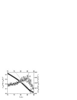
FIG. 3.: Microwave surface impedance data for $\lambda_{ab}^{2}\left(T=0\right)/\lambda_{ab}^{2}\left(T\right)$ and $d\left(\lambda_{ab}^{2}\left(T=0\right)\right/\lambda_{ab}^{2}\left(T\right))/dT$ versus $T$ of a high-quality Bi₂Sr₂CaCu₂O_8+δ single crystal taken from Jacobs et al. [13]. The solid line is $\lambda_{ab}^{2}\left(T=0\right)/\lambda_{ab}^{2}\left(T\right)=1.25\left(1-T/T_{c}\right)^{2/3}$ with $T_{c}=87.5$K, the dash-dot line its derivative, indicating the behavior of the homogeneous bulk system, and the dashed line is the tangent at the inflection point, $T_{p_{c}}\approx 87$K.

To substantiate the occurrence of a finite size effect and to clarify whether or not the rather small $L_{c}$ value is associated with a different shape of the superconducting domains and different boundary conditions, we derived and display in Fig.4 the finite size scaling function. The parameters entering this derivation are listed in Table I. Although the curve adopts the generic shape, in analogy to the film data shown in Fig.3, there is an essential difference. Indeed, $g_{0c}=1.6$, entering Eq.(18), differs substantially from the film value $g_{0c}=0.6$.

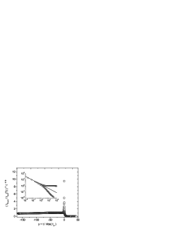
FIG. 4.: Finite size scaling function $g$ versus $t/\left|t_{p_{c}}\right|$ for the in-plane penetration depth data shown in Fig.3, derived from the data of Jacobs et al.[13].The insert shows the log plot and the solid lines are Eq.(18) with $g_{0c}=1.6$.

To provide some hints concerning the extrinsic or intrinsic nature of the inhomogeneities, we consider next the data taken on a high quality optimally doped Bi₂Sr₂CaCu₂O_8+δ single crystal of different provenance. In Fig.5 we displayed the data for the sample with $T_{c}=91$K, obtained with the single coil inductance method[14]. In analogy to the data shown in Figs.1 and 3 there is clear evidence for a rounded transition, giving rise to an inflection point. Invoking the finite size scaling analysis outlined above and the parameters listed in Table I (SC2) we obtain with Eq.(6) for the limiting length along the c-axis the estimate $L_{c}\simeq 80$Å. Although the data is not very dense around $T_{c}$, the resulting scaling function shown in Fig.6 is consistent with the expected behavior of the finite size scaling function. The solid lines are Eq.(18) with $g_{0c}=1.2$.

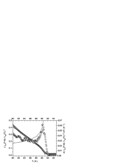
FIG. 5.: Single coil inductance data for $\lambda_{ab}^{2}\left(T=0\right)/\lambda_{ab}^{2}\left(T\right)$ and $d\left(\lambda_{ab}^{2}\left(T=0\right)/\lambda_{ab}^{2}\left(T\right)\right)/dT$ versus $T$ of a high-quality Bi₂Sr₂CaCu₂O_8+δ single crystal taken from Di Castro et al. [14]. The solid line is $\lambda_{ab}^{2}\left(T=0\right)/\lambda_{ab}^{2}\left(T\right)=1.9\left(1-T/T_{c}\right)^{2/3}$with $T_{c}=91$K, the dashed line its derivative, indicating the behavior of the homogeneous bulk system.

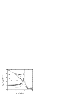
FIG. 6.: Finite size scaling function $g$ versus $t/\left|t_{p_{c}}\right|$ for the in-plane penetration depth data shown in Fig.5. The insert shows the log plot and the solid lines are Eq.(18) with $g_{0c}=1.2$.

Summarizing the in-plane penetration depth data taken on three Bi₂Sr₂CaCu₂O_8+δ films and two single crystals, we uncovered in all these samples clear evidence for a finite size effect, stemming from the tail in the temperature dependence of the in-plane penetration depth. We have shown that the scaling behavior of this tail is fully consistent with a finite size effect, arising from the finite extent of the superconducting domains along the c-axis (see Figs.2, 4 and 6). Noting that in these five samples $L_{c}$ is of nanoscale and varies from $68$ to $137$ Åonly, it is suggestive to trace the occurrence of domains back to an intrinsic phenomenon. Furthermore, from Table I it is seen that the $g_{0c}$ value of the films differs substantially from that of the single crystals. Since $g_{0c}$ depends on the shape of the superconducting domains and the boundary conditions at their surface, it becomes clear that the inhomogeneities in the films differ in an essential manner from those in single crystals. Moreover, given the estimates for $g_{0c}$, $\xi_{0ab}^{t}$and $L_{c}$, $g_{0c}\xi_{0ab}^{t}/L_{c}$ is readily calculated. The resulting estimates provide an independent check of the consistency of the finite size scaling analysis. Indeed, according to Eq.(15), this quantity should equal $\left(\lambda_{0ab}\left(0\right)/\lambda_{ab}\left(T_{c}\right)\right)^{2}$. In Table I we observe satisfactory consistency.

To substantiate the generic occurrence of the finite size effect we turn to the data taken on magnetic field c-axis aligned YBa₂Cu₃O_6.7 powder, where both, the temperature dependence of the in-plane and out of plane penetration depths, have been measured[15]. In Fig.7 we displayed respectively, $\left(1/\lambda_{ab}\left(T\right)\right)^{2}$, $d\left(1/\lambda_{ab}\left(T\right)\right)^{2}/dT$ versus $T$ and $d\left(1/\lambda_{ab}\left(T\right)/\lambda_{c}\left(T\right)\right)/dT$ versus $T$. The solid lines are respectively, $\left(1/\lambda_{ab}\left(T\right)\right)^{2}=\left(1/\lambda_{0ab}\right)^{2}\left|t\right|^{2/3}$ and $1/\lambda_{ab}\left(T\right)/\lambda_{c}\left(T\right)=1/\left(\lambda_{0ab}\lambda_{0c}\right)\left|t\right|^{2/3}$, while the dashed lines are the respective derivatives. These lines indicate the leading critical behavior of the homogeneous system. The corresponding values for $T_{c}$ and the critical amplitude $1/\left(\lambda_{0ab}\lambda_{0c}\right)$ are listed in Table II, while the parameters of the finite size scaling analysis are summarized in Table III. Here we used Eqs.(6) and (7) to obtain the estimates for $L_{c}$ and $L_{ab}$, the diameters of the superconducting domains. While $L_{c}$ is comparable to the values found in Bi₂Sr₂CaCu₂O_8+δ (see Table I), $L_{ab}$ turns out to be an order of magnitude larger. Its value $L_{ab}=592$Åis consistent with the lower bound $L_{ab}>576$Å, derived from the magnetic field induced finite size effect on the specific heat of YBa₂Cu₃O_6.6[11].

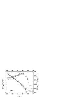
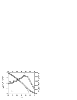
FIG. 7.: (a) $\left(1/\lambda_{ab}\left(T\right)\right)^{2}$ $\left(\bigcirc\right)$ and $d\left(1/\lambda_{ab}\left(T\right)\right)^{2}/dT$ $\left(\square\right)$ versus $T$ for YBa₂Cu₃O_6.7 derived from the data of Panagopoulos et al.[15]. The solid lines is $\left(1/\lambda_{ab}\left(T\right)\right)^{2}=\left(1/\lambda_{0ab}\right)^{2}\left|t\right|^{2/3}$ and the dashed line its derivative, indicating the leading critical behavior of the homogeneous system. The corresponding values for $T_{c}$ and the critical amplitude $\left(1/\lambda_{0ab}\right)^{2}$ are listed in Table II; (b) $1/\lambda_{ab}\left(T\right)/\lambda_{c}\left(T\right)$ $\left(\bigcirc\right)$ and $d\left(1/\lambda_{ab}\left(T\right)/\lambda_{c}\left(T\right)\right)/dT$ $\left(\square\right)$ versus $T$ for YBa₂Cu₃O_6.7 derived from the data of Panagopoulos et al.[15]. The solid line is $1/\lambda_{ab}\left(T\right)/\lambda_{c}\left(T\right)=1/\left(\lambda_{0ab}\lambda_{0c}\right)\left|t\right|^{2/3}$ and the dashed one its derivative, indicating the leading critical behavior of the homogeneous system. The corresponding values for $T_{c}$ and the critical amplitude $1/\left(\lambda_{0ab}\lambda_{0c}\right)$ are listed in Table II, while the parameters resulting from the finite size scaling analysis are summarized in Table III.

$T_{c}$	$\left(\lambda_{0ab}\right)^{-2}$	$\left(\lambda_{0ab}\lambda_{0c}\right)^{-1}$	$\left(\lambda_{0c}\right)^{-2}$	$\gamma$	$\left(\lambda_{ab}\left(T_{c}\right)\right)^{-2}$	$\left(\lambda_{ab}\left(T_{c}\right)\lambda_{c}\left(T_{c}\right)\right)^{-1}$	$\left(\frac{\lambda_{0ab}}{\lambda_{ab}\left(T_{c}\right)}\right)^{2}$	$\frac{\lambda_{0ab}\lambda_{0c}}{\lambda_{ab}\left(T_{c}\right)\lambda_{c}\left(T_{c}\right)}$
(K)	$\left(\mu\text{m}\right)^{-2}$	$\left(\mu\text{m}\right)^{-2}$	$\left(\mu\text{m}\right)^{-2}$		$\left(\mu\text{m}\right)^{-2}$	$\left(\mu\text{m}\right)^{-2}$
61.5	18.5	1.4	0.11	13.2	0.874	0.076	0.047	0.054

Table II: Estimates for $T_{c}$, $\left(\lambda_{0ab}\right)^{-2}$, $\left(\lambda_{0ab}\lambda_{0c}\right)^{-1}$, $\lambda_{0c}$, $\gamma=\lambda_{0c}/\lambda_{0ab}$, $\lambda_{ab}\left(T_{c}\right)$ and $\lambda_{ab}\left(T_{c}\right)\lambda_{c}\left(T_{c}\right)$ for YBa₂Cu₃O_6.7 derived from the data shown in Figs.7.

$T_{p_{c}}$	$T_{p_{ab}}$	$\left(\frac{1}{\lambda_{ab}\left(T_{p_{c}}\right)}\right)_{T_{p_{c}}}^{2}$	$\left(\frac{1}{\lambda_{ab}\left(T\right)\lambda_{c}\left(T\right)}\right)_{T_{p_{ab}}}$	$L_{c}$	$L_{ab}$	$\xi_{0ab}^{t}$	$\sqrt{\xi_{0ab}^{t}\xi_{0c}^{t}}$	$g_{0c}$	$\frac{g_{0c}\xi_{0ab}^{t}}{L_{c}}$	$g_{0ab}$	$\frac{g_{0ab}\sqrt{\xi_{0ab}^{t}\xi_{0c}^{t}}}{L_{ab}}$
(K)	(K)	$\left(\mu\text{m}\right)^{-2}$	$\left(\mu\text{m}\right)^{-2}$	(Å)	(Å)	(Å)	(Å)
59.66	59.3	1.85	0.16	52	592	5	64.3	0.5	0.05	0.55	0.06

Table III: Finite size scaling estimates for YBa₂Cu₃O_6.7 derived from the data shown in Figs.7.

(( (a) $\left|t\right|^{-\nu}\left(\lambda_{0ab}/\lambda_{ab}\left(T\right)\right)^{2}$ versus $t/\left|t_{p_{c}}\right|$ and (b) $\left|t\right|^{-\nu}\left(\left(\lambda_{0ab}\lambda_{0c}\right)/\left(\lambda_{ab}\left(T\right)\lambda_{c}\left(T\right)\right)\right)$ versus $t/\left|t_{p_{ab}}\right|$ derived from the data shown in Fig.7 for YBa₂Cu₃O${}_{6.7}.$ ))

To complete the finite size scaling analysis and the evidence for superconducting domains with diameters $L_{c}$ and $L_{ab}$, we displayed in Fig.8 the scaling functions $\left|t\right|^{-\nu}\left(\lambda_{0ab}/\lambda_{ab}\left(T\right)\right)^{2}$ versus $t/\left|t_{p_{c}}\right|$ and $\left|t\right|^{-\nu}\left(\left(\lambda_{0ab}\lambda_{0c}\right)/\left(\lambda_{ab}\left(T\right)\lambda_{c}\left(T\right)\right)\right)$ versus $t/\left|t_{p_{ab}}\right|$. Together with Eqs.(13) to (14) we observe the required agreement with the behavior of the respective finite size scaling function. The near coincidence $g_{0c}\simeq g_{0ab}\simeq 0.5$ implies nearly identical shape and boundary condition along the c-axis and the ab-plane. Moreover, $g_{0c}\simeq 0.5$ is close to the value in the Bi₂Sr₂CaCu₂O_8+δ films (Table I). To provide a consistency check of the finite size scaling analysis we note that, given the estimates for $g_{0k}$, $\sqrt{\xi_{0i}^{t}\xi_{0j}^{t}}$ and $L_{k}$, the quantity $g_{0k}\sqrt{\xi_{0i}^{t}\xi_{0j}^{t}}/L_{k}$ is readily calculated and should be equal to $\left(\lambda_{0i}\lambda_{0j}\right)/\left(\lambda_{i}\left(T_{c}\right)\lambda_{j}\left(T_{c}\right)\right)$(Eq.(15)). Tables II and III reveal satisfactory agreement.

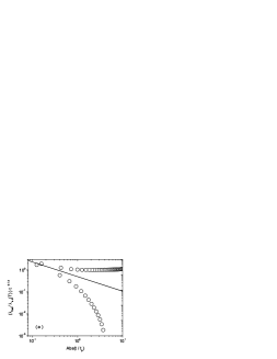
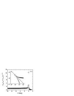
FIG. 8.: Finite size scaling function, (a) $\left|t\right|^{-\nu}\left(\lambda_{0ab}/\lambda_{ab}\left(T\right)\right)^{2}$ versus $t/\left|t_{p_{c}}\right|$ and (b) $\left|t\right|^{-\nu}\left(\left(\lambda_{0ab}\lambda_{0c}\right)/\left(\lambda_{ab}\left(T\right)\lambda_{c}\left(T\right)\right)\right)$ versus $t/\left|t_{p_{ab}}\right|$ derived from the data shown in Fig.7 for YBa₂Cu₃O_6.7 with the parameters listed in Table III. The insert shows the log plot.

To summarize, we have shown that the tail in the temperature dependence of the in-plane and out of plane penetration depth around $T_{c}$, as observed in the experimental data considered here, is fully consistent with a finite size effect, arising from homogeneous nanoscale superconducting domains with diameters $L_{ab}$ and $L_{c}$. Clearly this finite size effect is not restricted to the penetration depth but should be visible in other thermodynamic properties, including the specific heat, as well. In the specific heat it leads to a rounding of the peak and its consistency with a finite size effect was established for the data taken on YBa₂Cu₃O_7-δ high quality single crystals[17, 20]. In these samples the domain size was found to range from 300 to 400 Å. Although the investigations of Gauzzi et al.[21] on YBa₂Cu₃O_6.9 films with reduced long-range structural order clearly reveal that the size of the domains depends strongly on the growth conditions, we established their nanoscale size and their thermodynamic relevance in a variety of samples.

We thank K. D. Osborn et al. for providing their experimental data.

REFERENCES

[1] G. Bednorz and K. A. Müller, Z. Phys. B 64, 189
(1986).
[2] J. Mesot, P. Allensbach, U. Staub, and A. Furrer, Phys. Rev.
Lett. 70, 865 (1993).
[3] A. Furrer et al., Physica C 235-240, 261
(1994).
[4] J. Liu, J. Wan, A. Goldman, Y. Chang, and P. Jiang, Phys.
Rev.Lett. 67, 2195 (1991).
[5] A. Chang, Z. Rong, Y. Ivanchenko, F. Lu, and E. Wolf, Phys.
Rev. B 46, 5692 (1992).
[6] T. Cren, D. Roditchev, W. Sacks, J. Klein, J.-B. Moussy, C.
Deville-Cavellin, and M. Laguës, Phys. Rev. Lett. 84,
147 (2000).
[7] K. M. Lang, V. Madhavan, J. E. Hoffman, E. W. Hudson, H.
Eisaki , S. Uchida, and J. C. Davis, Nature 415, 413
(2002).
[8] Ch. Renner and Ø. Fischer, Phys. Rev. B 51,
9208 (1995).
[9] T. Schneider, cond-mat/0302024.
[10] D. Di Castro, G. Bianconi, M. Colapietro, A.
Pifferi, N.L. Saini, S. Agrestini, and A. Bianconi, Eur. Phys. J. B
18, 617 (2000).
[11] T. Schneider, cond-mat/0210702.
[12] K. D. Osborn, D. J. Van Harlingen, Vivek Aji, N.
Goldenfeld, S. Oh, and J. N. Eckstein, cond-mat/0204417.
[13] T. Jacobs, S. Sridhar, Q. Li, G. D. Gu, and N. Koshizuka,
Phys. Rev. Lett. 75, 4516 (1995).
[14] D. Di Castro, N.L. Saini, A. Bianconi, and A. Lanzara,
Physica C 332, 405 (2000).
[15] C. Panagopoulos, J. R. Cooper, and T. Xiang, Phys.Rev. B
57, 13422 (1998).
[16] M. E. Fisher and M. N. Barber, Phys. Rev. Lett. 28, 1516 (1972).
[17] T. Schneider and J. M. Singer, Phase Transition
Approach To High Temperature Superconductivity, Imperial College
Press, London, 2000.
[18] N. Schultka and E. Manousakis, Phys. Rev. B 52,
7528 (1995).
[19] R. Prozorov et al., cond-mat/0007013.
[20] T. Schneider, Physica B 326, 289 (2003).
[21] A. Gauzzi et al., Europhys.Lett., 51, 667 (2000).