Density Matrix Renormalisation Group Calculations for Two-Dimensional Lattices: An Application to the Spin-Half and Spin-One Square-Lattice Heisenberg Models

Abstract

A new density matrix renormalisation group (DMRG) approach is presented for quantum systems of two spatial dimensions. In particular, it is shown that it is possible to create a multi-chain-type 2D DMRG approach which utilises previously determined system and environment blocks at all points. One firstly builds up effective quasi-1D system and environment blocks of width $L$ and these quasi-1D blocks are then used to as the initial building-blocks of a new 2D infinite-lattice algorithm. This algorithm is found to be competitive with those results of previous 2D DMRG algorithms and also of the best of other approximate methods. An illustration of this is given for the spin-half and spin-one Heisenberg models on the square lattice. The best results for the ground-state energies per bond of the spin-half and spin-one square-lattice Heisenberg antiferromagnets for the $N=20\times 20$ lattice using this treatment are given by $E_{g}/N_{B}=-0.3321$ and $E_{g}/N_{B}=-1.1525$, respectively.

PACS numbers: 75.10.Jm, 75.50Ee, 03.65.Ca

I Introduction

The subject of one-dimensional lattice quantum spin systems at zero-temperature contains a large number of exact solutions, for example, via the Bethe Ansatz solution ba1 ; ba2 ; ba3 ; ba4 . However, such exact solutions have not as yet been universally obtained for systems of quantum spin number, $s\geq 1/2$, or for lattices of larger than one spatial dimension, or indeed for frustrated spin systems. It is noted however that exact solutions for such systems do exist for various specialised cases. Recent density matrix renormalisation group (DMRG) calculations dmrg1 have been extremely useful in determining the ground- and excited-state properties of a whole host of one-dimensional (1D) or quasi-1D spin systems to extremely high accuracy. The DMRG method is not limited by the magnitude of the quantum spin number or by the presence of frustration, and DMRG has been used to determine the non-zero temperature and dynamical properties of many quantum systems.

It is perhaps still fair to say that the full power of the DMRG method has largely been restricted to one-dimensional systems, although recent calculations have very successfully extended dmrg_2D_1 ; dmrg_2D_2 ; dmrg_2D_3 ; dmrg_2D_999 ; dmrg_2D_4 ; dmrg_2D_5 ; dmrg_2D_6 previous DMRG calculations for one-dimensional quantum systems to two spatial dimensions (2D). Perhaps the simplest such 2D DMRG approach is the “multi-chain” approach dmrg_2D_1 ; dmrg_2D_2 ; dmrg_2D_3 ; dmrg_2D_5 in which, during the infinite-lattice algorithm, ones keeps the width of the lattice constant and then one grows the lattice height by adding whole rows or partial rows of sites. The multi-chain finite-lattice algorithm may then be implemented and one repeatedly sweeps through all lattice sites until a fixed point of the renormalisation group (RG) process is reached. This is in direct analogy with the traditional one-dimensional algorithm, and so (in some sense) one has mapped the 2D problem onto an effective 1D problem. This multi-chain approach has been seen to work well for relatively small-sized lattices in Ref. dmrg_2D_5 in which whole lines of sites are added at a time. Indeed, a “finite-lattice sweep” was performed after each addition of a line of sites (and not just after the final $N=L\times L$ lattice had been created) in this calculation dmrg_2D_5 , and this was seen to greatly enhance the accuracy of the method.

Another approach dmrg_2D_4 was to split the two-dimensional lattice into four pieces, namely, two-dimensional system and environment blocks separated by a lines of spins which itself was split into distinct blocks, namely, one-dimensional system and environment blocks, and free spin(s). This “four block” approach is a truly two-dimensional algorithm in the sense that one is able to grow the two-dimensional lattice in a controlled manner using the results (i.e., 1D and 2D blocks) of previous iterations and a lattice of arbitrary size may be thus finally obtained. However, this approach suffers from a number of problems such as, for example, the need to diagonalise very large density matrices for the two-dimensional blocks for relatively modest numbers of states. We also note that these density matrices for the 2D blocks may also be highly singular.

Another recent and very successful 2D DMRG dmrg_2D_5 approach used two blocks at opposite corners of a square lattice with two “free” spins placed at particular positions along the boundary between the system and environment blocks. It was seen for this method that there was no need to set the width of the lattice to be constant and that previously defined blocks for a given $N=L\times L$ lattice could be used in the following DMRG iterations to form lattices of size $N^{\prime}=L+1\times L+1$. Furthermore, this approach was found to be very efficient for the (relatively small) lattices ($N=L\times L$ with $L\leq 12$) considered, and excellent results for the ground-state energy per bond of the spin-half Heisenberg model on the square and triangular lattices were obtained. An application of the DMRG method for highly anisotropic two-dimensional systems was also recently performed dmrg_2D_6 .

In this article a new 2D algorithm is presented which builds up two-dimensional lattices in a fast, simple and efficient manner. Quasi-1D blocks of up to a given length, $L$, are determined and thereafter the width is kept constant – in analogy with previous multi-chain approaches. However, these quasi-1D blocks are then used to form the first initial steps of an algorithm which uses 2D blocks of various shape and which have been determined during earlier DMRG steps in order to finally build up a lattice of size $N=L\times L$. Lattices of arbitrary size may thus be considered, although this ‘size’ is pre-set at the start of the DMRG calculation. This is in marked contrast to previous multi-chain approaches. The 2D “finite-lattice” DMRG algorithm has also been implemented here in order to arrive at a fixed point of the renormalisation group process, and this part of the algorithm is similar (if not identical) to previous multi-chain algorithms.

Note that the details of the DMRG approach are deferred until the appendix. However, it is important to note that the current approach does not utilise a row of sites or partial row in order to build up the lattice in the infinite-lattice algorithm. Rather, it does use previously defined blocks for the environment block which have both width and height at all points. The total system size is thus incremented by more than a single line of sites at a time, although the width is kept constant.

II The Heisenberg model for the square lattice

The Heisenberg model is given by

$$H=\sum_{\langle i,j\rangle}{\bf s}_{i}~{}\cdot~{}{\bf s}_{j}~{}~{},$$ (1)

and where ${\langle i,j\rangle}$ runs over each nearest-neighbour bond on the square lattice (counting each bond once and once only) and open boundary conditions are assumed. The results of the best of other approximate methods for the spin-half case qmc4 ; series1 ; swt ; ccm1 predict that $E_{g}/{N_{B}}\approx-0.3347$ (where $N_{B}$ is the number of bonds) and that 61-62% of the classical ordering remains for the quantum system in the infinite-lattice limit, $N\rightarrow\infty$. The results of the best of other approximate methods for the spin-one case series1 ; ccm2 predict that $E_{g}/{N_{B}}\approx-1.164$ (where $N_{B}$ is the number of bonds) and that 80-81% of the classical ordering remains for the quantum system in the infinite-lattice limit.

III Results

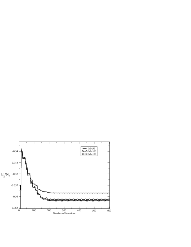
Figure 1: The DMRG ground-state energies per bond of the spin-half Heisenberg on a $N=6\times 6$ square lattice for $M=\{50,100,150\}$. Note that each “iteration” indicates a 2D DMRG “move” described in detail in the appendix. Note that the infinite-lattice algorithm ends after 22 iterations (close to the peak in the $E_{g}/N_{B}$) and the results thereafter refer to those for the finite-lattice algorithm.

A plot of the ground-state energy per bond for the $s=1/2$ Heisenberg antiferromagnet for the $N=6\times 6$ lattice for $M=\{50,100,150\}$ is presented in Fig. 1. It is seen that the trend of the ground-state energy is to decrease with the number of iterations and the minimal solution is quickly reached. Note however that edge effects are seen where, for example, the ground-state energy is slightly lower for moves 1-3 of the algorithm presented above. Also, the infinite-lattice algorithm ends after 22 “moves” indicated on the abscissa as “iterations” in Fig. 1 and we note that the ground-state energy per bond has a peak at this point. Thus, the finite-lattice algorithm reduces the ground-state energy per bond by about 6% to 8%. Slightly larger gains (up to about 10%) from the finite-lattice algorithm are possible for the larger lattices.

A value for the ground-state energy is taken from one of the sites near to the centre of the 2D square lattice for all of the $N=L\times L$ lattices considered here. By contrast, it is noted that the number of iterations needed to obtain convergence increases strongly with increasing $N$. It is observed that the number of iterations necessary can be as large as 20000 or more for $L=12$ and $L=20$. Indeed, it was seen that the ground-state energy sometimes decreases in a step-like fashion (even after 10000 or more iterations large step-like changes were sometimes observed). An example of this is given in a plot of the ground-state energy per bond for the $s=1$ Heisenberg antiferromagnet for the $N=12\times 12$ lattice for $M=\{50,100,150\}$ of Fig. 2. It would be interesting to test whether such step-wise changes occur for other 2D DMRG algorithms and if this were a characteristic of implementing the DMRG method in two spatial dimensions. Finally, an explicitly assumption of these simulations was that they had been run long enough in order to reach the RG fixed-point.

Note that the infinite-lattice algorithm ends after about 80 “moves” in Fig. 2 (which are again indicated on the abscissa as “iterations”) and we note that the ground-state energy per bond has a peak at this point. Thus, the finite-lattice algorithm reduces the ground-state energy per bond by about 8% to 10%.

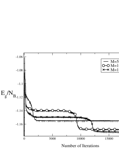
Figure 2: The DMRG ground-state energies per bond of the spin-one Heisenberg on a $N=12\times 12$ square lattice for $M=\{50,100,150\}$. Note that each “iteration” indicates a 2D DMRG “move” described in detail in the appendix. Note that the infinite-lattice algorithm ends at the peak in $E_{g}/N_{B}$ and the results thereafter refer to those for the finite-lattice algorithm.

These results may also be compared to results of previous DMRG calculations dmrg_2D_5 in Tab. 1 for the spin-half Heisenberg model on square lattices of varying size. Two algorithms were used in Ref. dmrg_2D_5 , which were, namely, a 2D algorithm in which the 2D system and environment blocks are grown from the corners and a multi-chain approach (also described in Refs. dmrg_2D_1 ; dmrg_2D_2 ; dmrg_2D_3 ) in which whole lines of sites were added at a time during the infinite-lattice approach. The results of these approaches shall henceforth be referred in this article to as DMRG (a) and DMRG (b) results, respectively, and the results of the present approach using the infinite-lattice algorithm shall be referred to as DMRG (c) results.

It is seen from Tab. 1 that we obtain reasonable correspondence between the present DMRG (c) results and the previous DMRG (a) and (b) results for all the lattices considered. A simple ‘heuristic’ extrapolation of these results in the limit $M\rightarrow\infty$ by assuming that the ground-state energy scales as a “power-law” with respect to $M$, which ought to be the case for a gapless system. The best fit of such a power-law dependence was determined and the extrapolated values were determined. Note that this simple treatment gave an extrapolated value for the ground-state energy per bond of $E_{g}/N_{B}=-0.36219$ for the $N=6\times 6$ lattice. This result is in good agreement with the extrapolated value for the ground-state energy of the spin-half square-lattice Heisenberg antiferromagnet of Ref. dmrg_2D_5 , namely, $E_{g}/N_{B}=-0.36212$. The extrapolated result for the ground-state energy per bond of the spin-half antiferromagnet on the $N=20\times 20$ lattice is given by $E_{g}/N_{B}=-0.3321$. This result for the $N=20\times 20$ lattice is in reasonable agreement with the results of the best of other approximate methods qmc4 ; series1 ; swt ; ccm1 . These methods predict that $E_{g}/{N_{B}}\approx-0.3347$ in the infinite-lattice limit, $N\rightarrow\infty$, and note that this result ought to be quite close to the result of the $N=20\times 20$ lattice, even with closed boundary conditions. (Note that no extrapolations of the 2D DMRG results in the limit $N\rightarrow\infty$ were determined due to the small number of data points and the fact that a relatively large lattice was considered anyway, although such an extrapolation is possible to perform.)

Table 1: DMRG results for the ground-state energy per bond of the spin-half Heisenberg antiferromagnet on the square lattice for lattices of size $N=L\times L$ with $L=\{6,12,20\}$ and for number of DMRG states $M=\{50,100,150\}$. The new results are referred to as DMRG (c) results and these results are compared to two previous DMRG two-dimensional approaches (see Ref. dmrg_2D_5 ) referred to as DMRG (a) and DMRG (b) results, respectively. It is seen that the present DMRG results are in reasonable agreement with these previous 2D DMRG results – especially for the $N=12\times 12$ lattice.

	$N$	$M=50$	$M=100$	$M=150$
DMRG (a)	$6\times 6$	$-$0.361972	$-$0.362096	–
DMRG (b)	$6\times 6$	$-$0.361919	$-$0.362089	–
DMRG (c)	$6\times 6$	$-$0.35847	$-$0.36135	$-$0.36184
DMRG (a)	$12\times 12$	$-$0.337374	$-$0.341588	–
DMRG (b)	$12\times 12$	$-$0.332574	$-$0.338833	–
DMRG (c)	$12\times 12$	$-$0.33260	$-$0.33757	$-$0.33984
DMRG (c)	$20\times 20$	$-$0.31763	$-$0.32441	$-$0.32679

Results for the spin-one Heisenberg model are also shown in Tab. 2 for square lattices of size $N=12\times 12$ and $N=20\times 20$. These these results were again extrapolated in the limit $M\rightarrow\infty$ and we obtained an extrapolated result of $E_{g}/N_{B}=-1.1525$ for the spin-one antiferromagnet on the $N=20\times 20$ lattice. This result for $N=20\times 20$ the lattice is seen to be in modest agreement with those results of the best of other approximate methods series1 ; ccm2 for both the ground-state energy per bond, evaluated in the limit $N\rightarrow\infty$, namely, $E_{g}/{N_{B}}\approx-1.164$.

It may also be seen from Tab. 1 that the DMRG (a) results of the 2D algorithm of Ref. dmrg_2D_5 appear to perform better in terms of the ground-state energy per bond of the spin-half Heisenberg model than either the DMRG (b) and the present DMRG (c) approaches for all of the lattices considered. It is thus interesting to consider why different DMRG approaches for exactly the same model and lattice at equivalent levels of approximation yield differing results. It is known global1 from the simulation of one dimensional chains with periodic boundary conditions that the ground state does not become fully translationally invariant, thus indicating that the “global minimum” obtained may be somewhat dependent on the build up considered. However, even for the same topological buildup and the same final number of states kept, the outcome may depend qualitatively on which way the number of states kept was increased during the sweeping process of the finite-lattice algorithm global2 .

Table 2: New DMRG results for the ground-state energy per bond of the spin-one Heisenberg antiferromagnet on the square lattice for lattices of size $N=L\times L$ with $L=\{12,20\}$ and for number of DMRG states $M=\{50,100,150\}$. The DMRG results are compared to those results of SWT series1 , cumulant series expansions series1 , and the CCM ccm2 for the infinite-lattice limit.

	$N$	$E_{g}/N_{B}$
DMRG(c) $M=50$	$12\times 12$	$-$1.15472
DMRG(c) $M=100$	$12\times 12$	$-$1.16780
DMRG(c) $M=150$	$12\times 12$	$-$1.1715
DMRG(c) $M=50$	$20\times 20$	$-$1.10654
DMRG(c) $M=100$	$20\times 20$	$-$1.13939
DMRG(c) $M=150$	$20\times 20$	$-$1.1462
CCM	$\infty$	$-$1.1646
SWT	$\infty$	$-$1.1641
Series Expansions	$\infty$	$-$1.16395(1)

IV Conclusions

In this article a new density matrix renormalisation group (DMRG) algorithm was presented which determines the properties of two-dimensional square-lattice spin-half and spin-one Heisenberg antiferromagnets. This algorithm builds up 2D lattices of arbitrary size in a straightforward manner, and, although conceptually similar to earlier multi-chain approaches for 2D lattices, the method differs from these earlier approaches in practice because one firstly builds up effective quasi-1D system and environment blocks of width $L$. These quasi-1D blocks were then used to form the initial steps of a infinite-lattice algorithm in order to build a lattice of arbitrary, although (as for the 1D DMRG algorithm) preset at the start of the calculation, size. It has thus been proven that it is possible to construct a multi-chain DMRG approach for 2D lattices which uses previously determined system and environment blocks at all points.

This new 2D DMRG approach tested for the spin-half and spin-one square-lattice Heisenberg models in order to predict their ground-state energies with great success. The best results for ground-state energy of the square-lattice Heisenberg model for the $N=20\times 20$ lattice for the spin-half and spin-one models were found $E_{g}/N_{B}=-0.3321$ and $E_{g}/N_{B}=-1.1525$. The results for the Heisenberg model on the $N=6\times 6$ and $N=12\times 12$ were found to be a reasonable agreement with both previous DMRG results for the spin-half square-lattice model dmrg_2D_5 with $M=50$ and $M=100$. Furthermore, the new DMRG results for the $N=20\times 20$ lattice were seen to be in reasonable agreement with the results of the best of other approximate methods qmc4 ; series1 ; swt ; ccm1 ; ccm2 determined in the limit $N\rightarrow\infty$. These new results, and those results of previous and highly successful DMRG calculations in 2D dmrg_2D_1 ; dmrg_2D_2 ; dmrg_2D_3 ; dmrg_2D_4 ; dmrg_2D_5 , now show that the DMRG method is quickly becoming a powerful tool in order to simulate and understand strongly interacting two-dimensional quantum many-body systems.

Future 2D DMRG calculations for the spin-half and spin-one Heisenberg models are envisaged for even larger square lattices and for larger values for $M$. Other future calculations using the new DMRG approach could also be for the spin-half and spin-one Heisenberg models on the triangular and Kagomé lattices. Indeed, extensions of the approach presented in this article to lattice quantum spin systems with frustrating next-nearest-neighbour bonds are also possible. It is finally noted that the 2D algorithms considered in this article may be applied to a wide range of both fermionic and bosonic systems.

Acknowledgement: I wish to gratefully acknowledge and to thank Ulrich Schollwöck for his strong support in writing this article and for his invaluable help and advice in performing DMRG calculations.

Appendix A Density Matrix Renormalisation Group (DMRG) Algorithm for two spatial dimensions

Figure 3: The one-dimensional system block is the lower block of sites and it is used to initialise the infinite-lattice algorithm. The “free” spins $S1$ and $S2$ are indicated by the unfilled circles and the environment is the upper block (chain) of sites. Diagram (a) thus shows a one-dimensional system block $(6,1)$ of width $l_{1D}(=6)$ and of height $1$. Figure (b) shows the system block $(7,2)$ which is of width $L(=9)$ and height $2$. (Note that the differently shaped blocks are uniquely described by the indices $(x,y)$ shown above.)

The method of building up the 2D lattice is now introduced and the first step in this algorithm is to build up one-dimensional lattices of width $L$ and height of one and two sites (shown in Fig. 3). These blocks are used as the initial starting point for the two-dimensional infinite-lattice algorithm. Note that each differently shaped block in Fig. 3 is uniquely described by the indices $(x,y)$, as shown in the figure and that this labelling of the differently shaped blocks is crucial to this 2D implementation of the DMRG algorithm. System blocks are thus uniquely denoted by the indices $x$ and $y$, where $x$ which refers to the right-most site for the $y$-th “row” of sites from the bottom of the system block. By comparison, the index $x$ represents the $x$-th left-most site for the $y$-th “row” of sites from the top of the environment block in this case. Thus, system and environment blocks with the same indices refer to block shapes which are related by a transformation of a rotation of 180^∘ (about some arbitrary central point).

The density matrix for the free spin $S1$ and the system block is obtained by integrating out the degrees of freedom of the other spin $S2$ and the environment block. The new Hamiltonian and spin operators are then determined in terms of this “augmented block” of the system block and its neighbouring spin $S1$. All of the information regarding these system blocks of shape ($x$,$y$) (for example, the number of states, the Hamiltonian, and the spin operators) is saved to disk for both of bottom and top blocks. This information is used later in order to start the full 2D lattice infinite-lattice algorithm. Hence, note that one firstly grows the width of the lattice until it reaches a preset size $L$ and height 1, as shown in Fig. 1a. One then ‘sweeps’ from the left to the right such that the free spins S2 and S1 run along the top of the ladder-like structure shown in Fig. 1b. The quasi-2D blocks are now of height 2 and the process is stopped once the spin S2 lies on the left-most site.

Figure 4: The first step in the infinite-lattice approach. Note that the positions of the sites in the bottom-most row of the environment block are reversed from left to right. “Free” spins $S1$ and $S2$ are again indicated by the unfilled circles.

In the first truly two-dimensional “step,” the system block of index $(x,y)=(1,L)$ is copied into the environment block, although the ordering of the sites on the bottom row of the environment block are reversed such that sites in the environment block run from $L,~{}L-1,~{}\cdots,~{}1$, shown in Fig. 4 for $l_{2D}=2$. The reason why one perhaps ought to do this is because it is hoped that it is beneficial to use a block of width $L$ in order to retain the maximum number of bonds between the system and environment block (namely, $L$ of them). Note that the system block is denoted by indices $(3,2)$ (again see Fig. 4).

Presumably, the symmetries of this “reversed” block are slightly different from that of the unreversed case, and so this choice of environment block it is not ideal. However, the goal of this approach is to use previously defined blocks in order to quickly build up the final lattice in order for the finite-lattice algorithm to find the fixed-point of the RG process. However, note that that there may exist many alternate ways of performing this crucial “first step” and more is said of this below. Now that the first two-dimensional step has been described in detail it is possible to present the full algorithm. Note that we start from step 2 after defining the initial step mentioned above for the augmented block $(2,2)$ and that the density matrix for the system block and spin $S1$ and the relevant Hamiltonian and spin operators obtained for this augmented block are stored to disk at all points. The ‘steps’ in the 2D algorithm is now given by:

Figure 5: The second such “step” in the infinite-lattice approach. Note new system block determined in the previous step, namely (2,$l_{2D}$), is used in both the system and environment blocks.

1. The system block of index $(x,y)=(l_{2D}-1,L)$ is now copied into the environment block and the ordering of the sites on the bottom row of the environment block are reversed such that sites in the environment block run from $L,~{}L-1,~{}\cdots,~{}1$, shown in Fig. 4. The two “free” spins are put at positions $(1,l_{2D})$ and $(2,l_{2D})$ and the system block is defined by the left-most site in the second row, namely, block $(x,y)=(3,l_{2D})$. The density matrix for the system block and the spin $S1$ is obtained and the effective Hamiltonian and spin operators determined. The results are then saved for both the top and bottom blocks of this shape of the augmented block, namely, $(x,y)=(2,l_{2D})$.

2. The next 2D “step” shown in Fig. 5 uses system and environment blocks both indexed by $(2,l_{2D})$, although the sites in the bottom row of the environment block are not reversed in this case. Again, the density matrix for the system block and the spin $S1$ is obtained and the effective Hamiltonian and spin operators determined. This information is saved to disk for the augmented block(s) given by $(1,l_{2D})$.

3. In the next step the system block is referred to by the index $(1,l_{2D})$ and the environment block by $(3,l_{2D})$, as is shown in Fig. 6. The value of $l_{2D}$ is now incremented. For example, after the routine which determines the initial 1D blocks (see Fig. 3) has been completed then $l_{2D}$ is increment from a value of 2 to 3.

4. The fourth type of “step” (or, more accurately stated, a set of steps) is in one in which one “sweeps” through values of $l_{1D}=\{1,2,~{}\cdots,~{}L-3\}$, shown in Fig. 7 . The density matrices are determined at each step and the information for the system block $(x,y)=(l_{2D},l_{1D})$ for both the top bottom 2D blocks is saved.

Clearly, the four types of different step described above may be used in an analogous way in order to sweep leftwards. (Note however that one starts from step 1 from now on). Furthermore, the final $N=L\times L$ lattice is formed by repeatedly sweeping right and then left, and so on. Thereafter the information stored to disk may be used in order to implement a finite-lattice algorithm in which one sweeps through all lattice sites repeatedly until a fixed point of the RG process is reached. It is furthermore noted that prediction of the wave function is possible for both the infinite-lattice and the finite-lattice algorithms, and that this can reduce the number of Lanczös iterations by up to an order of magnitude.

Figure 6: The third “step” in the infinite-lattice approach.

It is hoped that this method might, in principle, allow one to add in the degrees of freedom associated with the spin $S1$ into new 2D blocks in a very controlled and efficient manner. Furthermore, it is hoped that the use of effective system and environment blocks at all points might to help in simulating the effects of the surrounding lattice spins on these free spins – which might be especially pronounced for larger lattices.

The infinite-algorithm presented here is, perhaps, one of the simplest 2D algorithms which utilises previously defined fully 2D blocks in order to build up the 2D lattice. The research presented in this article (and that also presented in Ref. dmrg_2D_5 ) however conclusively proves that one may construct DMRG infinite-lattice algorithms which utilise previously defined 2D blocks at all points. Note however that more elegant solutions which also contain this property might be constructed using similar ideas, as mentioned above. For example, an environment block of shape $(1,l_{2D}-2)$ might be used in step 1 of the 2D algorithm presented here. Another alternative is to use a line of spins (or partial line of spins), which would be necessary for step 1 only. Both of these alternatives to the ‘step 1’ used above would obviate the need to reverse the ordering of the lattice sites on the bottom on the environment block in this step.

Figure 7: The fourth and final set of “steps” infinite-lattice approach. The arrow shows the direction of the sweeping and note that $l_{1D}$ runs over all indices $\{1,2,~{}\cdots,~{}L-3\}$.

Note again that the Heisenberg Hamiltonian is given by Eq. (1) and that we wish to solve the Schrödinger equation, $H|\Psi\rangle=E_{g}|\Psi\rangle$, where $|\Psi\rangle$ is the superblock ground-state wave function. The Hamiltonian may also be broken into distinct parts, given by

$$H \equiv H_{\rm system}+H_{\rm system,S1}+H_{\rm system,S2}$$ (2)

$$+ H_{\rm system,environment}+H_{\rm environment}$$

$$+ H_{\rm environment,S2}+H_{\rm environment,S2}~{}~{}.$$

It is noted that (by far) the largest amount of computational time is spent evaluating $H_{\rm system,environment}|\Psi\rangle$ during each Lanczös iteration. Indeed, the number of operations involved in determining this scales as $LM{{}^{4}}$, where $M$ is the number of states retained at each DMRG iteration.

All system/environment interaction terms for the $L$ distinct bonds between the system and environment blocks are determined and the gathered together before the Lanczös algorithm is invoked, and this information is then saved to local (RAM) memory. The number of operations involved in determining system/environment interactions is thus reduced by a factor of $L$, although the memory usage is commensurately increased by a factor of $M^{4}$ which puts a limit on the maximum number of the states $M$. Note that future calculations will distribute this memory usage up by the use of parallel processing, such that each processor which on a given part of the whole system block/environment block interactions. This not only reduces the memory usage of each individual machine but also considerably speeds up the DMRG algorithm.

Furthermore, the data for the lower and upper two-dimensional blocks for indices $(x,y)$ is also saved to disk. This is because the memory required to store all of the information for the spin operators scales with $L^{3}M^{2}$ which again very quickly becomes prohibitive. However, as this data is read from disk once per DMRG iteration, this approach is not too inefficient. The problem of system/environment block interactions appears to be present in all 2D implementations of the DMRG method in 2D and so an efficient implementation of these terms is crucial to a good DMRG code.

References

- (1) H. A. Bethe, Z. Phys. 71, 205 (1931).
- (2) L. Hulthén, Ark. Mat. Astron. Fys. A 26, No. 11 (1938).
- (3) R. Orbach, Phys. Rev. 112, 309 (1958); C. N. Yang and C. P. Yang, ibid. 150, 321 (1966); ibid. 150, 327 (1966).
- (4) J. Des Cloiseaux and Pearson, Phys. Rev. 128, 2131 (1962); L. D. Faddeev and L. A. Takhtajan, Phys. Lett. 85A, 375 (1981).
- (5) S.R. White and R. Noack, Phys. Rev. Lett. 68, 3487 (1992); S.R.White, Phys. Rev. Lett. 69, 2863 (1992); S.R.White, Phys. Rev. B 48 10345 (1993).
- (6) S.R. White, Phys. Rev. Lett. 77, 3633 (1996).
- (7) R. Noack and S.R. White, in “Density-Matrix Renormalisation: A New Numerical Method In Physics,” edited by I. Pechsel et al., Lecture Notes in Physics, Vol. 528 (Springer-Verlag, Heidelberg, Berlin, 1998), p. 27.
- (8) R.M. Noack, S.R. White, and D.J. Scalapino, in “Computer Simulations in Condensed Matter Physics VII,” edited by D.P. Landau, K.K. Mon, and H.B. Schüttler, (Springer-Verlag, Berlin, 1994).
- (9) T. Xiang, Phys. Rev. B 53, R10445 (1996).
- (10) P. Henelius, Phys. Rev. B 60, 9561 (1999).
- (11) T. Xiang, J. Lou, and Z. Su, Phys. Rev. B 64, 104414 (2001).
- (12) S. Moukouri and L.G. Caron, cond-mat/0210668.
- (13) A.W. Sandvik, Phys. Rev. B 56, 11678 (1997).
- (14) R.F. Bishop, D.J.J. Farnell, and J.B. Parkinson, Phys. Rev. B 61, 6775 (2000).
- (15) W. Zeng, J. Oitmaa, and C. J. Hamer, Phys. Rev. B 43, 8321 (1991).
- (16) C.J. Hamer, W.H. Zheng, and P. Arndt, Phys. Rev. B 46, 6276 (1992).
- (17) R.F. Bishop, D.J.J. Farnell, S.E. Krueger, J.B. Parkinson, J. Richter, and C. Zeng, J. Phys.: Condens. Matter 12, 7601 (2000).
- (18) D.J.J. Farnell, R.F. Bishop, and K.A. Gernoth, Phys. Rev. B 64, 172409 (2001).
- (19) T. Nishino, in “Density-Matrix Renormalisation: A New Numerical Method In Physics,” edited by I. Pechsel et al., Lecture Notes in Physics, Vol. 528 (Springer-Verlag, Heidelberg, Berlin, 1998), p. 127.
- (20) U. Schollwöck – in preparation.