Bulk Mediated Surface Diffusion: The Infinite System Case

Abstract

An analytical soluble model based on a Continuous Time Random Walk (CTRW) scheme for the adsorption-desorption processes at interfaces, called bulk-mediated surface diffusion, is presented. The time evolution of the effective probability distribution width on the surface is calculated and analyzed within an anomalous diffusion framework. The asymptotic behavior for large times shows a sub-diffusive regime for the effective surface diffusion but, depending on the observed range of time, other regimes may be obtained. Montecarlo simulations show excellent agreement with analytical results. As an important byproduct of the indicated approach, we present the evaluation of the time for the first visit to the surface.

I Introduction

The dynamics of adsorbed molecules is a fundamental issue in interface science v1 ; v4 and is crucial to a number of emerging technologies v1 ; v5 . Its role is central to phenomena as diverse as foam relaxation v6 and the evolution of blood protein deposit v7 . Recently, the mechanism called bulk-mediated surface diffusion has been identified and explored. Its importance in relaxing homogeneous surface density perturbations is experimentally well established. This mechanism arises at interfaces separating a liquid bulk phase and a second phase which may be either solid, liquid, or gaseous. Whenever the adsorbed species is soluble in the liquid bulk, adsorption-desorption processes occur continuously. These processes generate a surface displacement because molecules desorb, undergo Fickian diffusion in the bulk liquid, and are then re-adsorbed elsewhere. When this process is repeated many times, it results in an effective diffusion of a molecule on the surface. Bichuk and OShaughnessy Bichuk have claimed that this effective surface diffusion has anomalous super-diffusive characteristics when certain range of time is considered.

Dynamical processes that display anomalous diffusion Tsallis ; Prato ; Re ; Zasla ; Klafter ; Blumen ; Zumofen have been characterized by a non linear time dependence of the mean square displacement of the walker for long times; that is $\langle r^{2}(t)\rangle\;\sim\;t^{\epsilon}$ with $\epsilon\;\neq 1$ (remember that $\epsilon=1$ corresponds to normal diffusion) since $\langle r^{2}\rangle$ is the usual estimator of the square width of the probability distribution at time $t$. Hence, for anomalous diffusion we have that the probability distribution width grows faster (slower) for $\epsilon>1$ ($\epsilon<1$) than it does for normal diffusion.

In this paper we present an analytical soluble model for the adsorption-desorption processes based on a Continuous Time Random Walk (CTRW) scheme. We calculate the evolution with time of the square width of the effective probability distribution on the surface and show that, for a given range of time, this square width growth as $t^{\epsilon}$ where $\epsilon$ depends on the values of the adsorption and diffusion parameters.

II The adsorption-desorption model

Let us start with the problem of a particle making a random walk in the semi-infinite cubic lattice. The position of the walker is defined by the vector $\vec{r}$ whose components are denoted by the integer numbers $n,m,l\geq 1$ corresponding to the directions $x$, $y$ and $z$ respectively. The displacements in the $x$ and $y$ directions are unbounded. In the $z$ direction the particle can move from $l=1$ to infinity.

The probability that the walker is in $(n,m,l)$ at time $t$, given that it was at $(0,0,l_{0})$ at $t_{0}$, $P(n,m,l;t|n,m,l_{0};t_{0})\equiv P(n,m,l;t)$, satisfies the following set of coupled master equations

$$\dot{P}(n,m,1;t) = \gamma P(n,m,2;t)-\delta P(n,m,1;t),~{}~{}~{}~{}~{}~{}~{}~{}~{}~{}~{}~{}~{}~{}~{}~{}~{}~{}~{}~{}~{}~{}~{}~{}~{}~{}~{}~{}~{}~{}~{}~{}~{}~{}\mbox{ $l=1$}$$

$$\dot{P}(n,m,2;t) = \alpha[P(n-1,m,2;t)+P(n+1,m,2;t)-2P(n,m,2;t)]+$$

$$\beta[P(n,m-1,2;t)+P(n,m+1,2;t)-2P(n,m,2;t)]+$$

$$\gamma P(n,m,3;t)+\delta P(n,m,1;t)-2\gamma P(n,m,2;t),~{}~{}~{}~{}~{}~{}~{}~{}~{}~{}~{}~{}\mbox{ $l=2$}$$

$$\dot{P}(n,m,l;t) = \alpha[P(n-1,m,l;t)+P(n+1,m,l;t)-2P(n,m,l;t)]+$$ (1)

$$\beta[P(n,m-1,l;t)+P(n,m+1,l;t)-2P(n,m,l;t)]+$$

$$\gamma[P(n,m,l+1;t)+P(n,m,l-1;t)-2P(n,m,l;t)],~{}~{}~{}~{}\mbox{ $l\geq 3$}$$

where $\alpha,\beta$ and $\gamma$ are the transition probabilities per unit time in the $x$,$y$ and $z$ directions respectively, and $\delta$ is the desorption probability per unit time from the boundary plane defined by $z=1$.

Taking the Fourier transform with respect to the $x$ and $y$ variables and the Laplace transform with respect to the time $t$ in the above equations, we obtain

$$sG(k_{x},k_{y},1;s)-P(k_{x},k_{y},1,t=0) = \gamma G(k_{x},k_{y},2;s)-\delta G(k_{x},k_{y},1;s),~{}~{}~{}~{}~{}~{}~{}\mbox{ $l=1$}$$

$$sG(k_{x},k_{y},2;s)-P(k_{x},k_{y},2,t=0) = A(k_{x},k_{y})G(k_{x},k_{y},2;s)+\delta G(k_{x},k_{y},1;s)+$$

$$\gamma G(k_{x},k_{y},3;s)-2\gamma G(k_{x},k_{y},2;s),~{}~{}~{}~{}~{}\mbox{ $l=2$}$$

$$sG(k_{x},k_{y},l;s)-P(k_{x},k_{y},l,t=0) = A(k_{x},k_{y})G(k_{x},k_{y},l;s)+$$ (2)

$$\gamma[G(k_{x},k_{y},l-1;s)+$$

$$G(k_{x},k_{y},l+1;s)-2G(k_{x},k_{y},l;s)],~{}~{}~{}\mbox{ $l\geq 3$}$$

We have used the following definitions

$$G(k_{x},k_{y},l;s|0,0,l_{0};t_{0}) = \int_{0}^{\infty}e^{-st}\sum_{n,m=-\infty}^{\infty}e^{k_{x}n+k_{y}m}P(n,m,l;t|n,m,l_{0};t_{0})dt$$ (3)

$$= \mbox{}L[\sum_{n,m=-\infty}^{\infty}e^{k_{x}n+k_{y}m}P(n,m,l;t|n,m,l_{0};t_{0})],$$

where $L$ indicates the Laplace transform of the quantity within the brackets, and

$$A(k_{x},k_{y})=2\alpha[Cos(k_{x})-1]+2\beta[Cos(k_{y})-1].$$ (4)

It is possible to write Eq. (II) in matrix form as

$$[u\tilde{I}-\tilde{H}]\tilde{G}=\delta_{ll_{0}}=\tilde{I}_{ll_{0}},$$ (5)

where the square matrix $\tilde{G}$ has components

$$\tilde{G}_{ll_{0}}=[G[k_{x},k_{y},l;s|n,m,l_{0};t_{0}]],$$ (6)

In Eq. (5), $\tilde{I}$ is the identity matrix and $\tilde{H}$ is a three-diagonal matrix with the following form

$$\tilde{H}=\left(\begin{array}[]{cccccc}-\delta&\gamma&0&0&0&\cdots\\ \delta&C&\gamma&0&0&\cdots\\ 0&\gamma&C&\gamma&0&\cdots\\ 0&0&\gamma&C&\gamma&\cdots\\ \cdot&\cdot&\cdot&\cdot&\cdot&\cdots\\ \end{array}\right),$$

and $C$ is defined as

$$C=-2\gamma+A(k_{x},k_{y}).$$ (7)

In order to find the solution to the Eq. (5), we decompose the $\tilde{H}$ matrix in the following way

$$\tilde{H}=A(k_{x},k_{y})\tilde{I}+\tilde{H}_{0}+\tilde{H}_{1}+\tilde{H}_{2},$$ (8)

where

$$\tilde{H}_{0}=\left(\begin{array}[]{cccccc}-2\gamma&\gamma&0&0&0&\cdots\\ \gamma&-2\gamma&\gamma&0&0&\cdots\\ 0&\gamma&-2\gamma&\gamma&0&\cdots\\ 0&0&\gamma&-2\gamma&\gamma&\cdots\\ \cdot&\cdot&\cdot&\cdot&\cdot&\cdots\\ \end{array}\right),$$

$$(\tilde{H}_{1})_{ij}=\Delta_{1}\left\{\begin{array}[]{ll}1&\mbox{if i = j = 1}\\ 0&\mbox{otherwise}\end{array}\right.$$

$$(\tilde{H}_{2})_{ij}=\Delta_{2}\left\{\begin{array}[]{ll}1&\mbox{if i = 1 and j = 2}\\ 0&\mbox{otherwise}\end{array}\right.$$

with

$$\Delta_{1} = -\delta-[-2\gamma+A(k_{x},k_{y})],$$

$$\Delta_{2} = \delta-\gamma.$$ (9)

Defining

$$\tilde{G}^{0} = [(s-(A(k_{x},k_{y}))\tilde{I}-\tilde{H}_{0})]^{-1},$$

$$\tilde{G}^{1} = [(s-(A(k_{x},k_{y}))\tilde{I}-\tilde{H}_{0}-\tilde{H}_{1})]^{-1},$$ (10)

observing that a formal solution of Eq. (5) is

$$\tilde{G}=[s\tilde{I}-\tilde{H}]^{-1},$$ (11)

and by reiterating the Dyson formula, we can show that

$$\tilde{G}_{ll_{0}}=\tilde{G}^{1}_{ll_{0}}+\frac{\Delta_{2}\tilde{G}^{1}_{l2}\tilde{G}^{1}_{1l_{0}}}{1-\Delta_{2}\tilde{G}^{1}_{12}},$$ (12)

$$\tilde{G}^{1}_{ll_{0}}=\tilde{G}^{0}_{ll_{0}}+\frac{\Delta_{1}\tilde{G}^{0}_{l1}\tilde{G}^{0}_{1l_{0}}}{1-\Delta_{1}\tilde{G}^{0}_{11}}.$$ (13)

The form for $\tilde{G}^{0}_{ll_{0}}$ can be obtained by conventional methods vanKampen as

$$\tilde{G}^{0}_{ll_{0}}=L(e^{2\gamma t}(I_{|j-j_{0}|}(2\gamma t)-I_{|j+j_{0}|}(2\gamma t)))_{\tilde{u}},$$ (14)

where $I_{n}(2\gamma t)$ is the first modified Bessel function of order $n$. The above expression points out that the Laplace transform is evaluated at the argument $\tilde{u}=[s-A(k_{x},k_{y})]$.

Once the general expression for $\tilde{G}$ is obtained, we can find the probability that a particle is on the plane at site $(m,n,l=1)$ at time $t$ given it was at $(0,0,l=1)$ at $t=0$. This probability may be obtained using the inverse Laplace transform in $s$ and the inverse Fourier transform on $k_{x}$, $k_{y}$ of the matrix element $\tilde{G}_{11}$.

A direct measurable experimental magnitude Bichuk is the variance of the probability distribution at time $t$ over the plane $z=1$

$$<r^{2}(t)>_{plane},$$ (15)

which measures the spreading of particles over this plane. Once $P(m,n,l=1;t|0,0,l_{0}=1;t=0)$ is known, the variance is calculated as:

$$<r^{2}(t)>_{plane}=\sum_{m,n=-\infty}^{\infty}P(m,n,l=1;t|0,0,l_{0}=1;t_{0})(m^{2}+n^{2}).$$ (16)

Here, we have used symmetry properties for the diffusion along the $x$ and $y$ axes, that is $<x(t)>=<y(t)>=0$.

The Laplace transform of the variance $<r^{2}(s)>_{plane}=L(<r^{2}(t)>_{plane})$ can be found as follows

$$<r^{2}(s)>_{plane}=-[\frac{\partial^{2}}{\partial k_{x}^{2}}+\frac{\partial^{2}}{\partial k_{y}^{2}}][\tilde{G}_{11}]\mid_{k_{x}=k_{y}=0}$$ (17)

By using Eqs. (11) to (17), $<r^{2}(u)>_{plane}$ turns out to be the ratio of two complicated functions of $s$

$$<r^{2}(s)>_{plane}=\frac{N(s)}{D(s)},$$ (18)

where

$$N(s)=[4\delta\gamma(\alpha+\beta)][s^{2}(\sqrt{s(4\gamma+s)}-3s)+3\gamma^{2}(\sqrt{s(4\gamma+s)}-3s)-2\gamma^{3}],$$ (19)

and

$$D(s)=\sqrt{s(4\gamma+s)}(\gamma s(2\gamma+s-\sqrt{s(4\gamma+s)})+\delta(\gamma(\sqrt{s(4\gamma+s)}-3s)+s(\sqrt{s(4\gamma+s)}-s)))^{2}.$$ (20)

It is important to remark that the conservation of particles in the plane is not satisfied.

If we denote with $P_{plane}(t)$ the probability that the particle is in the plane $z=1$ at time $t$, it can be shown that the Laplace transform of the magnitude is

$$\tilde{P}_{plane}(s)=\frac{(\gamma(2\gamma+s-\sqrt{s(4\gamma+s)})}{(\gamma s(2\gamma+s-\sqrt{s(4\gamma+s)})+\delta(\gamma(\sqrt{s(4\gamma+s)}-3s)+s(\sqrt{s(4\gamma+s)}-s)))}.$$ (21)

In order to test the theoretical results for the $<r^{2}(t)>_{plane}$ and $P_{plane}(t)$, we have performed Montecarlo simulations for the adsorption-desorption processes obtaining an excellent agreement in both cases. Figures 1 and 2 show the variance and the probability that the particle is on the plane $z=1$ as a function of $t$, for three different values of $\delta$.

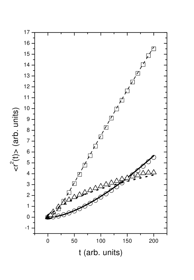
Figure 1: $<r^{2}(t)>$ vs time, for three different values of $\delta$. Circles correspond to simulations with $\delta=0.01$, while the solid line is the related theoretical curve. Squares are for simulations with $\delta=0.1$, and the dashed line is the theoretical curve. Triangles are for simulations with $\delta=1.0$, and the dotted line is the corresponding theoretical curve. In all figures we have used $\alpha=\beta=\gamma=1.0$, and the number of realizations is $10^{6}$.

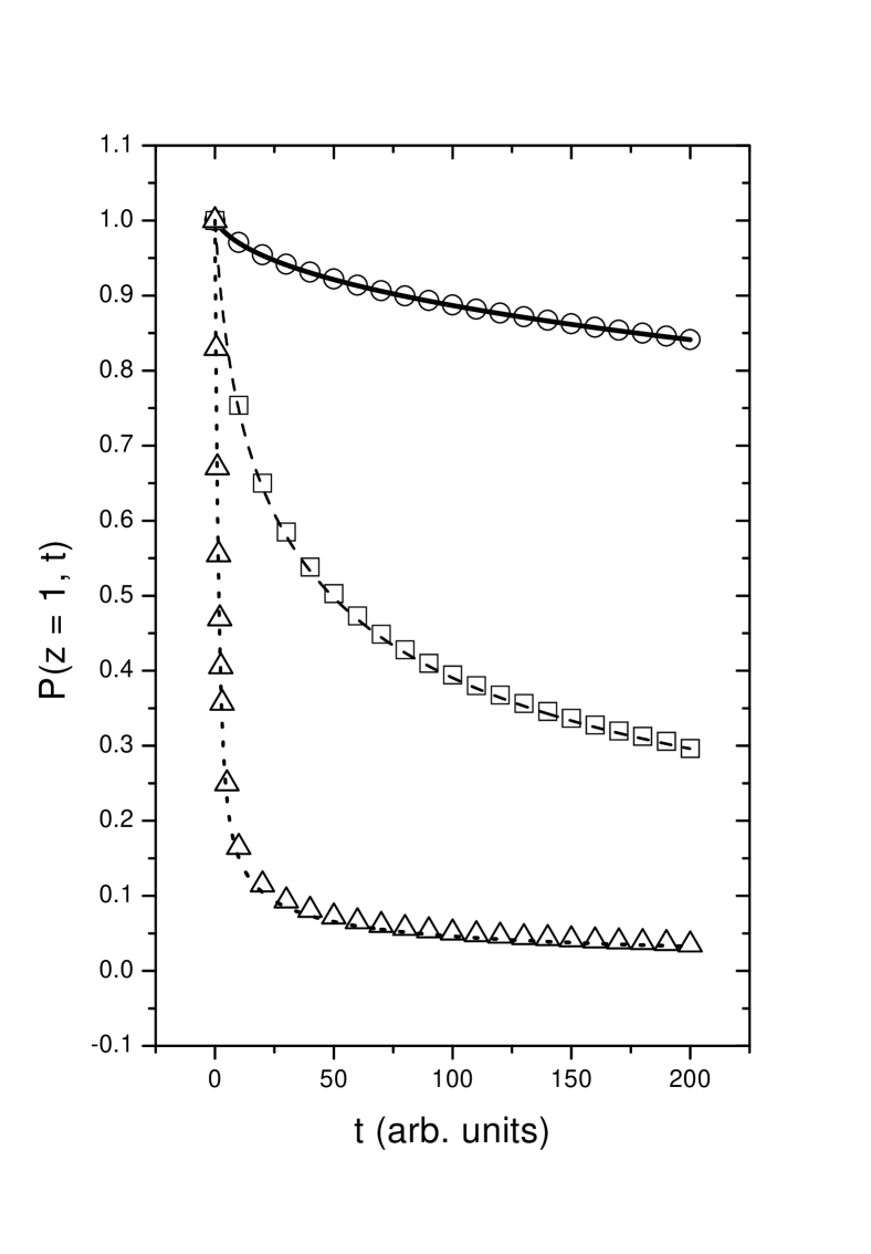
Figure 2: Probability $P(z=1;t)$ vs time, for three different values of $\delta$. Circles correspond to simulations with $\delta=0.01$, while the solid line is the theoretical curve. Squares are for simulations with $\delta=0.1$, and the dashed line is the theoretical curve. Triangles are for simulations with $\delta=1.0$, and the dotted line is the corresponding theoretical curve.

The asymptotic behavior for large $t$ of both, $<r^{2}(t)>_{plane}$ and $P_{plane}(t)$, can be obtained by means of Tauberian theorems Montroll as

$$<r^{2}(t)>_{plane}\rightarrow\frac{\sqrt{\gamma}}{\delta}\,\,\,\,\ \frac{(\alpha+\beta)}{\Gamma[3/2]}\,\,\,\,\ t^{\frac{1}{2}},$$ (22)

$$P_{plane}(t)\rightarrow\frac{\sqrt{\gamma}}{\delta}\,\,\,\,\ \frac{(\alpha+\beta)}{\Gamma[1/2]}\,\,\,\,\ t^{-\frac{1}{2}}.$$ (23)

From Eq. (22) we recognize an asymptotic sub-diffusive regime which is shown in Fig. 3.

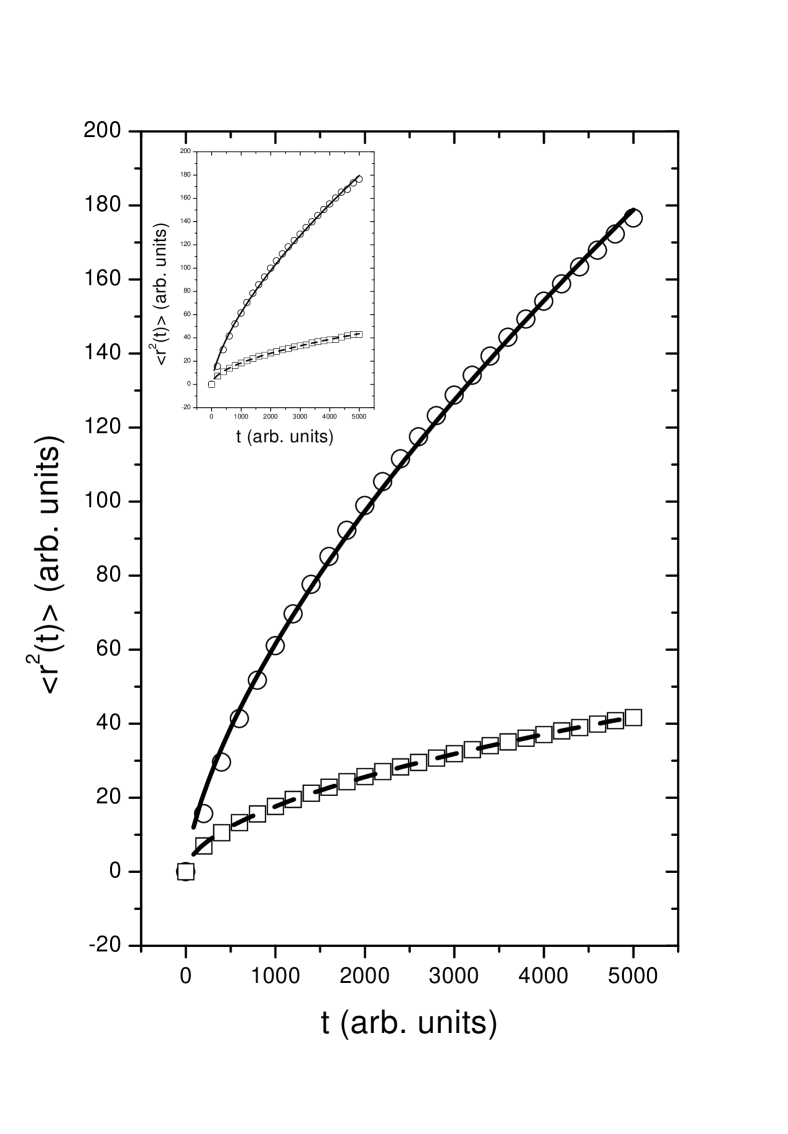
Figure 3: $<r^{2}(t)>$ vs time, for three different values of $\delta$, and compared with a fit using $y=at^{\epsilon}$. Circles correspond to theory with $\delta=0.01$, and the solid line to the fit with $a=0.63\pm 0.03$, $\epsilon=0.663\pm 0.007$. Squares are for theory with $\delta=0.1$, while the solid line is the fit with $a=0.435\pm 0.007$, $\epsilon=0.535\pm 0.005$. The insert shows the related results for simulations. Again circles correspond to $\delta=0.01$, and the solid line to the fit with $a=0.64\pm 0.04$ and $\epsilon=0.661\pm 0.008$; while squares are for $\delta=0.1$, and the solid line is the fit with $a=0.47\pm 0.01$, $\epsilon=0.531\pm 0.004$.

When we choose a different range of time in order to fit $<r^{2}(t)>_{plane}$ as $t^{\epsilon}$ we find that $\epsilon$ depends on the values of $\delta$ for fixed $\alpha,\beta$ and $\gamma$. Figure 4 shows this dependence for a wide range of values of the desorption rate $\delta$.

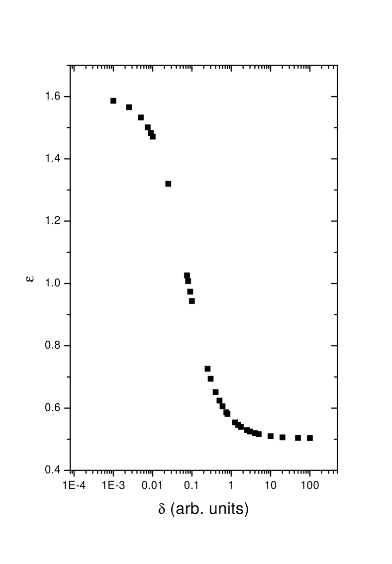
Figure 4: $\epsilon$ vs $\delta$, for time in the range $t=0$ to $t=500$. Note that for $\delta\rightarrow\infty$, $\epsilon$ approaches the value $0.5$, while for small values of $\delta$, $\epsilon$ becomes $\gg 1$.

III The CTRW Scheme

In this section we sumarize the most important results of the lattice CTRW approach. Let $\Psi(\vec{r},\vec{r^{\prime}};t)$ the waiting time density governing a single transition being defined as the probability density that a transition from $\vec{r^{\prime}}$ to $\vec{r}$ occurs at time between $t$ and $t+dt$ given the walker arrives at $\vec{r}$ at $t=0$. The transition time between different sites is assumed much shorter than the time spent at each lattice point; these ”instantaneous transitions” allow us to prove probability conservation as indicated below.

We assumed translational invariance, that is $\Psi(\vec{r},\vec{r^{\prime}};t)=\Psi(\vec{r}-\vec{r^{\prime}};t)$ for all $\vec{r}$ and $\vec{r^{\prime}}$, hence the conditional probability to find the particle at site $\vec{r}$ at time $t$ given it was at $\vec{r}=0$ at $t=0$, $P(\vec{r},t|\vec{r}=0,t=0)$ can be found in Laplace-Fourier variables $\vec{k}$ and $s$ as

$$P(\vec{k},s|\vec{r}=\vec{0};t=0)=\frac{1}{1-\tilde{\Psi}(\vec{k},s)}\,\,\frac{1-\tilde{\Psi}(s)}{s}$$ (24)

where $\tilde{\Psi}(\vec{k},s)$ is the Fourier-Laplace transform of $\Psi(\vec{r},t)$ and $\tilde{\Psi}(s)=\Psi(\vec{k}=\vec{0},s)$ is the Laplace transform of the total transition probability.

The normalization of $P(\vec{r},t|\vec{r}=\vec{0},t=0)$ for all $t$ is obtained from Eq. (24) in a direct way as

$$\sum_{\vec{r}}P(\vec{r};t|\vec{r}=\vec{0};t=0)=L^{-1}(\tilde{P}(\vec{k}=\vec{0},s|\vec{r}=\vec{0},t=0))=L^{-1}(\frac{1}{s})=1.$$ (25)

Normalization implies that the walker is somewhere in the (3D) lattice, but if we evaluate the probability that the walker is in a subspace of this lattice we will lose the normalization condition.

We now consider, as done previously Bichuk , the possibility that the successive visits of the walker to the plane $z=1$, as discussed in Section II, may be viewed as an CTRW over that plane. We must define a suitable waiting time density for single transitions, $\Psi_{plane}(\vec{r},\vec{r^{\prime}};t)$ where $\vec{r}$ and $\vec{r^{\prime}}$ are two dimensional vectors on the plane, i.e. $\vec{r}=(m,n)$ and $\vec{r^{\prime}}=(m^{\prime},n^{\prime})$. A transition between $\vec{r}$ and $\vec{r^{\prime}}$ must be done with no visit to the plane within the interval $(0,t)$, in order to be consistent with a single transition. If we remember that this waiting time density is the probability density that the walker arrives at $\vec{r}$ between $t$ and $t+dt$ having arrived at $\vec{r^{\prime}}$ at $t=0$, it is obvious that this transition is not instantaneous because the ”flying time” across the bulk cannot be neglected (see below). In order to be consistent with the CTRW theory we may consider that the particle remains at site $\vec{r^{\prime}}$ during this time and then perform a jump to the site $\vec{r}$. In this way, the probability over the plane is conserved and transitions become instantaneous.

Now we build up the waiting time density for this ”single transition” in the plane $z=1$, taking into account the above remarks. We note that if the walker has arrived at $(m^{\prime},n^{\prime},1)$ at $t=0$, the probability density to desorb from the plane per unit time around $t^{\prime}$ by a jump to $(m^{\prime},n^{\prime},2)$ is $\,\sim\delta\,\exp(-\delta t^{\prime})$. We define $q[(m,n,2),t;(m^{\prime},n^{\prime},2),t^{\prime}]$ as the probability of finding the walker at $(m,n,2)$ at time $t$ given it was in $(m^{\prime},n^{\prime},2)$ at time $t^{\prime}$ without visiting the plane $z=1$ in the interval $(t^{\prime},t)$. The probability density to reach $(m,n,1)$ for the first time between $t$ and $t+dt$ given the walker was in $(m^{\prime},n^{\prime},2)$ at time $t^{\prime}$ can be expressed as

$$f[(m,n,1),t;(m^{\prime},n^{\prime},2),t^{\prime})]=\gamma q[(m,n,2),t;(m^{\prime},n^{\prime},2),t^{\prime}].$$ (26)

Finally the density to reach $(m,n,1)$ for first time, per unit of time around $t$ given that the walker was in $(m^{\prime},n^{\prime},1)$ at $t=0$ without visiting the plane in the interval $(0,t)$ is:

$$f[(m,n,1),t;(m^{\prime},n^{\prime},1),0]=\int_{0}^{t}[\gamma q[(m,n,2),t;(m^{\prime},n^{\prime},2),t^{\prime}]]\delta\,\exp(-\delta t^{\prime})dt^{\prime}.$$ (27)

The function $f[(m,n,1),t;(m^{\prime},n^{\prime},1),t^{\prime}]$ plays the role of the waiting time density $\Psi_{Plane}(\vec{r},\vec{r^{\prime}};t)$ where $\vec{r}=(m,n)$ and $\vec{r^{\prime}}=(m^{\prime},n^{\prime})$. Since we are assuming translational invariance in the $x$ and $y$ directions, the function $q$ depends only on $(m-m^{\prime})$ and $(n-n^{\prime})$. Selecting $(0,0)$ as the starting point we obtain

$$\Psi_{plane}(m,n,t)=\int_{0}^{t}[\gamma q(m,n,2),t;(0,0,2),t^{\prime}]\delta\,\exp(-\delta t^{\prime})dt^{\prime}.$$ (28)

The function $q((m,n,2),t;(0,0,2),t^{\prime})$ is obtained by means of the method of images assuming an absorbent plane in $z=1$

$$q(m,n,2),t;(0,0,2),t^{\prime}) = [\exp(-2\alpha t)I_{m}(2\alpha t)]$$ (29)

$$[\exp(-2\beta t)I_{n}(2\beta t)]$$

$$[\exp(-2\gamma t)I_{0}(2\gamma t)-\exp(-2\gamma tI_{2}(2\gamma t)],$$

where $I_{j}$ is the modified Bessel function of order $j$. Equations (28) and (29) allow us to build the ”normalized probability” of the CTRW in the plane $z=1$

$$P^{norm}(\vec{r},t|\vec{r}=\vec{0},t=0)=L^{-1}F^{-1}\left(\frac{1}{1-\Psi_{plane}(\vec{k},s)}\right)\left(\frac{1-\Psi_{plane}(s)}{s}\right),$$ (30)

where

$$\Psi_{plane}(\vec{k},s)=\gamma(\frac{1}{2\gamma^{2}})(s+2\gamma+A(k_{x},k_{y})-\sqrt{(s+2\gamma-A(k_{x},k_{y})^{2}-(2\gamma)^{2}}))\frac{\delta}{s+\delta},$$ (31)

and $\Psi_{Plane}(s)=\Psi_{Plane}(\vec{k}=\vec{0},s)$. Here $\vec{r}=(m,n);\vec{k}=(k_{x},k_{y})$ and the function $A(k_{x},k_{y})$ is defined by Eq. (4). Eq. (31) shows a ”coupled” waiting time density with a divergent time first moment, that is $<t>\rightarrow\infty$.

Expressions for the Fourier-Laplace transform of $P^{norm}(\vec{r},t|\vec{r}=\vec{0},t=0)$ can be obtained from Eqs. (30) and (31).

$$P^{norm}(\vec{k},s|\vec{r}=\vec{0},t=0)=\frac{\frac{1}{s}(2\gamma(s+\delta)-\delta(s+2\gamma-\sqrt{s(s+4\gamma)}))}{2\gamma(s+\delta)-\delta(s+2\gamma+A(k_{x},k_{y})-\sqrt{(s+2\gamma+A(k_{x},k_{y}))^{2}-(2\gamma)^{2}})}.$$ (32)

The corresponding variance of $P^{norm}$ in Laplace space is

$$<r^{2}(s)>^{norm}=2\delta(\alpha+\beta)(\frac{2\gamma+s-\sqrt{s(s+4\gamma)}}{2\gamma s+\delta\sqrt{s(s+4\gamma)}-s}s\sqrt{s(s+4\gamma)}),$$ (33)

and the asymptotic behavior for large $t$ is

$$<r^{2}(t)>^{norm}\rightarrow(\alpha+\beta)\,t.$$ (34)

This result, i.e. normal diffusion, is due to the coupled character of the waiting time density Eq. (31), and its infinite time first moment.

As an important byproduct of the above approach, we present the evaluation of the probability of the first return to the plane $z=1$. If a walker, initially at the point $(0,0,1)$, desorbs and begins an excursion across the bulk, the probability density to return, for the first time, to the plane $z=1$ between $t$ and $t+dt$, $f_{ret}(t)$, is given by

$$f_{ret}(t)=L^{-1}[\Psi_{plane}(s)]=L^{-1}[\Psi_{plane}(\vec{k}=\vec{0},s)].$$ (35)

From the Eq. (31) we obtain the following expression the Laplace transform of the first return density

$$\Psi_{plane}(s)=(\frac{\delta}{2\gamma})(\frac{1}{s+\delta})(2\gamma+s-\sqrt{u(s+4\gamma)}).$$ (36)

We have made a numerical inverse transform of this result by using a numerical program and have compared this result with Montecarlo simulations finding an excellent agreement. See Fig. 5.

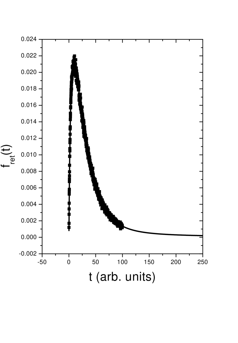
Figure 5: Distribution function for return times $f_{ret}(t)$ vs time for $\delta=0.5$. The squares correspond to simulations while the solid line is for theory.

Finally, from Eq. (36) it is possible to obtain two important results. Firstly, a walker is certain to return to the plane

$$\int_{0}^{\infty}f_{ret}(t)\,dt=\Psi_{plane}(s=0)=1.$$ (37)

Secondly, the asymptotic (long time) behavior of the first return density is

$$f_{ret}(t)\rightarrow(\frac{1}{\sqrt{\gamma}\,\,\,\ \Gamma[\frac{1}{2}]})\frac{1}{t^{\frac{3}{2}}},$$ (38)

indicating that the mean first time to return to the plane is infinite.

IV Conclusions

We presented in this paper an analytical model for the adsorption-desorption processes from a boundary plane in a semi-infinite cubic lattice. We studied the effective diffusion of molecules on this plane interface and calculated the evolution of the square width of the probability distribution. This square width can be fitted with a power law of $t$ whose exponent changes with the range of time considered and depends on the values of the adsorption and diffusion parameters. In this sense, effective anomalous super-diffusions reported by Bichuk and OShaughnessy Bichuk may be understood. However, in the asymptotic long time regime this square width always behaves as $t^{\frac{1}{2}}$. It is important to observe that the lack of probability conservation over the interface must be taken into account if a ”genuine” CTRW on the plane is considered as was pointed out in Section III. As a byproduct of our approach, we obtained the evaluation of the probability of the first return to the planar interface. We performed Montecarlo simulations of the adsorption-desorption process obtaining excellent agreement with the model predictions.

This work is part of a research project on bulk mediated diffusion on surfaces. Here we have discussed the case of infinite bulk while in nosotros1 we investigated the finite (in the direction normal to the surface) case where, among other aspects, we have found that an “optimal” number of layers exists, that produces the faster growth of $<r^{2}(t)>$. In addition, we have also investigated the case of non-Markovian desorption process nosotros2 where we have found an interesting oscillatory behavior. This research offers a more or less complete view of the theoretical description for the problem of bulk mediated diffusion on a surface.

Acknowledgments: The authors thank V. Grünfeld for a critical reading of the manuscript. HSW acknowledges the partial support from ANPCyT, Argentine, and thanks the MECyD, Spain, for an award within the Sabbatical Program for Visiting Professors, and to the Universitat de les Illes Balears for the kind hospitality extended to him.

References

- (1) J. H. Clint, Surfactant Aggregation (Chapman and Hall, New Jork, 1992).
- (2) H. E. Johnson, J. F. Douglas and S. Granick, Phys. Rev. Lett. 70 3267 (1993).
- (3) C.T. Shibata and A. M Lenhof, J. Colloid Interface Sci. 148, 469 (1992), 148, 485 (1992).
- (4) S. Kim and H. Y, J. Phys. Chem. 96, 4034 (1992).
- (5) Y. L. Chen, S. Chen, C. Frank and J. Israelachvili, J. Colloid Interface Sci. 153, 244 (1992).
- (6) A. A. Sonin, A. Bonfillon, and D. Langevin, Phys. Rev. Lett. 71, 2342 (1993).
- (7) A. L. Adams, G. C. Fishe, P. C. Munoz and L. Vroman, J. Biomed. Meter. Res. 18, 643 (1984).
- (8) O. Bichuk and B. O Shaughnessy, J. Chem. Phys., 101, 772 (1994). O. Bichuk and B. O Shaughnessy, Phys. Rev. Lett., 74, 1795 (1995). S. Stapf, R. Kimmich and R. O. Seitter, Phys. Rev. Lett., 75, 2855 (1995).
- (9) C. Tsallis, S.V.F. Levy, A.M.C. Souza and R. Maynard, Phys. Rev. Lett. 75, 3598 (1995). [Erratum: Phys. Rev. Lett. 27, 5442 (1996)].
- (10) D. Prato and C. Tsallis, Phys. Rev. E. 60, 2398 (1999).
- (11) M. A. Ré, C. E. Budde and D. P. Prato, Physica A, 323, 9 (2003).
- (12) G. M. Zaslavsky, Physica D, 76, 110 (1994).
- (13) J. Klafter, A. Blumen and M.F. Shlesinger, Phys. Rev. A 35, 3081 (1987).
- (14) A. Blumen, G. Zumofen and J. Klafter, Phys.Rev. A 40, 3964 (1989).
- (15) G. Zumofen, A. Blumen and M.F. Shlesinger, J. Stat. Phys.54, 1519 (1889).
- (16) N.G. Van Kampen, Stochastic Processes in Physics ans Chemistry, (North-Holland, Amsterdam, 1981).
- (17) E.W. Montroll and B.J. West, in Fluctuation Phenomena, E.W. Montroll and J.L. Lebowitz, eds. (North Holland, Amsterdam, 1979).
- (18) J.A. Revelli, C.E. Budde, D. Prato and H.S. Wio, Bulk Mediated Surface Diffusion: Finite System Case, to be submited.
- (19) J.A. Revelli, C.E. Budde, D. Prato and H.S. Wio, Bulk Mediated Surface Diffusion: Non Markovian Dynamics, to be submited.