Paradoxical games and Brownian thermal engines

Abstract

Two losing games, when alternated in a periodic or random fashion, can produce a winning game. This paradox occurs in a family of stochastic processes: if one combines two or more dynamics where a given quantity decreases, the result can be a dynamic system where this quantity increases. The paradox could be applied to a number of stochastic systems and has drawn the attention of researchers from different areas. In this paper we show how the phenomenon can be used to design Brownian or molecular motors, i.e., thermal engines that operate by rectifying fluctuations. We briefly review the literature on Brownian motors, pointing out that a new thermodynamics of Brownian motors will be fundamental to the understanding of most processes of energy transduction in molecular biology.

1 Paradoxical games

Suppose we have a biased coin, so that the probability that any flip will result in a head is $0.5-\epsilon$, where $\epsilon$ is a small and positive number. With this coin, call it coin 1, it is proposed that you play the following game: if the flip results in a tail you receive $1$ dollar, if not you pay the same amount. If you have unlimited capital then you should accept to play the game without hesitation: if $x(t)$ is your opponent’s capital after $t$ runs, it will not be difficult for you to show that its mean value, $\langle{x(t)}\rangle$ is a strictly a decreasing function of $t$ (while your average capital is an increasing function of $t$).

Now, it is proposed that you play a second game that uses two coins, call them coin $2$ and coin $3$ respectively. Coin $3$ is flipped whenever your opponent’s capital is a multiple of $3$, in any other case coin $2$ is flipped (note that your opponent can have negative capital; by a multiple of $3$ it is understood any integer number that can be written as $3n$, with $n$ an integer number). Let $p_{2}=0.75-\epsilon$ and $p_{3}=0.1-\epsilon$ be the probabilities that your opponent wins with coin $2$ and coin $3$ respectively, see Figure 1. The analysis of this game is not as simple as that of our previous game. However, it can be shown – see Appendix 1 and Figure 1 – that this game, too, is favourable for you in the sense that the mean value of the opponent’s capital $\langle{x(t)}\rangle$ is, once again, a strictly decreasing function of $t$. Let us call the first game we have described “game A” and the second one “game B.”

Once you are convinced that your opponent will lose in both games you are given a third proposal: alternate the games following the sequence AABBAABB… If you frown, the proposal can be modified to make it less suspicious: in each run we will randomly chose the game that is played. If you accept either of these proposals you would have trusted your intuition too much, not realizing that random systems, even as simple as the ones we have just described, may behave in an unexpected way.

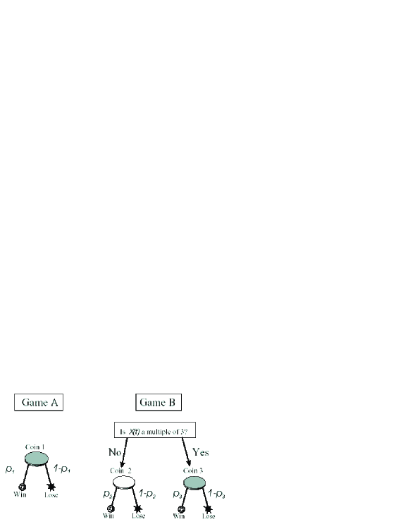
Figure 1: Rules of games A and B. The values of the probabilities are: $p_{1}=\frac{1}{2}-\epsilon$, $p_{2}=\frac{3}{4}-\epsilon$ and $p_{3}=\frac{1}{10}-\epsilon$, with $\epsilon$ small and positive, which in all cases favour the “losing” option. The lighter colour of coin $2$ indicates that with this coin the probability of winning is greater than $\frac{1}{2}$ and so it is a favourable coin.

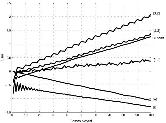
Figure 2: Average capital (over $50\,000$ players), as a function of the number of runs, for each of the games and in several combinations, including a random combination. In all cases $\epsilon=0.005$ and we have used the notation $[a,b]$ to indicate that we play $a$ runs of game A, followed by $b$ runs of game B, and so on. The random combination does not differ much from the combination $[2,2]$, that is, the combinaton AABBAA…(After [1]).

Indeed, if we alternate the games, either by following a fixed sequence AABBAABB… or chosing randomly the game we play, then your opponent’s average capital $\langle{x(t)}\rangle$ will be a strictly increasing function of $t$. Figure 2 shows your opponent’s capital in different situations: games A and B played alone, in several periodic combinations and in a random combination.

2 Detailed analysis of the games

The phenomenon we have just described is known as Parrondo’s paradox and it is receiving some attention [1, 2] because it is thought it might have application in areas such as economics and evolutionary theory. It is true that this phenomenon may arise in any situation that involves the interplay of two or more random dynamics. However, we have not yet described a real situation where the paradox takes place.

Let us see how we can analyse these paradoxical games. Game B and the random combination of games A and B may be reduced to a 3-state Markov chain [3]. These states are: the capital is multiple of $3$, multiple of $3$ plus $1$ or multiple of $3$ plus $2$. The variable that determines these states is

$$y\equiv x\hskip 8.5359pt\mathrm{mod}\,3$$ (1)

which only takes on the values $0$, $1$ and $2$. The analysis of this Markov chain can be carried out by diagonalizing a $3{\times}3$ matrix (see Appendix 1).

This analysis gives us the following intuitive explanation of the paradox. Game B uses two coins: one “bad”, coin $3$, and one “good”, coin $2$. When game B is played alone, the probability of using coin $3$ is

$$\pi_{0}=\frac{5}{13}-\frac{440}{2197}\epsilon+\ldots$$ (2)

where we have dropped the terms of order $\epsilon^{2}$ to simplify the analysis. Notice, also, that the probability $\pi_{0}$ is not equal to $\frac{1}{3}$, as one might have initially thought, but greater than $\frac{1}{3}$. Consequently, the probability of winning is

$$P_{\mathrm{win}}=\pi_{0}p_{3}+(1-\pi_{0})p_{2}=\frac{1}{2}-\frac{147}{169}\epsilon+\ldots$$ (3)

which is less than $\frac{1}{2}$ for any positive $\epsilon$. Nevertheless, when games A and B are combined randomly, the probability of using coin $3$ becomes

$$\pi^{\prime}_{0}=\frac{245}{709}-\frac{48880}{502681}\epsilon+\ldots$$ (4)

which is less than $\pi_{0}$. The probability of winning is now

$$P^{\prime}_{\mathrm{win}}=\pi^{\prime}_{0}\frac{p_{3}+p_{1}}{2}+(1-\pi^{\prime}_{0})\frac{p_{2}+p_{1}}{2}=\frac{727}{1418}-\frac{486795}{502681}\epsilon+\ldots$$ (5)

which is greater than $\frac{1}{2}$ if $\epsilon$ is small enough. What happens then is that game A, even though it consists of just one “bad” coin, redistributes the frequencies of use of the two coins of game B in such a way that the “good” coin is being used more often than its counterpart. This is the essence of the paradox: the winning tendency is already built-in into game B, but when this game is played alone, the losing tendency is dominant. The role of game A is to reverse this dominancy. Thus, game A, in spite of being a losing game, effects a reprise of the “good” coin of game B that overcomes its own losing tendency, so that the combination of games A and B becomes a winning game.

3 A simple Brownian motor

What has all this to do with physics? Even though now the paradox is part of probability theory, it was originally inspired by a physical system, namely, a Brownian motor or molecular motor [4, 5].

With a slight change in the winning and losing probabilities, the games described above could be interpreted as a Brownian particle in one-dimension subjected to certain potentials.

Let us consider the following model of a Brownian particle in one-dimension, where the particle can occupy the discrete set of positions $x=0,\pm 1\pm 2,\ldots$. The particle jumps with certain probability from one position to another at discrete times $t=0,1,2,...$ Suppose the particle is under the action of a certain periodic potential $V(x)$ of period $3$, i.e. $V(x+3)=V(x)$. This means the potential is completely defined by the three values: $V(0)$, $V(1)$ and $V(2)$, which we denote by $V_{0}$, $V_{1}$ and $V_{2}$, respectively. We will set $V_{0}=0$, $V_{1}=V$ and $V_{2}=\frac{V}{2}$, so that the potential is asymmetric (see Figure 3). In addition, suppose there is an external force $F$ acting on the particle and pointing to the left. The energy at each point is then

$$E(x)=V(x)+Fx.$$ (6)

How does this particle move at a certain temperature $T$? When a physical system is at a certain temperature $T$ and can be found in different states $i$ with energy $E_{i}$ its evolution may be described by a Markov chain [6]. The dynamics are expressed in terms of the transition probabilities $p(i\rightarrow j)$ for jumping from state $i$ to the state $j$. These probabilities must satisfy the detailed-balance condition. One of the dynamics to satisfy this requirement is the Metropolis algorithm (see Appendix 2) that is used in Monte-Carlo simulations of systems in equilibrium at a certain temperature $T$ [6].

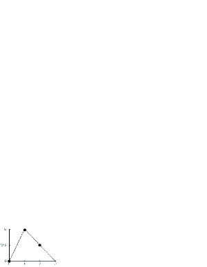
Figure 3: The potential used on the Brownian particle described in this article.

When our Brownian particle evolves following the Metropolis algorithm at a finite temperature $T$, its position $x(t)$ behaves more or less like the capital in game B. On the other hand, if we follow the Metropolis algorithm at a very high temperature, the resulting system is very much like game A. In both cases the external force plays the role of the games’ $\epsilon$ parameter. These analogies give us a strong indication how to reproduce the paradox in the behaviour of the Brownian particle. At any temperature the particle moves to the left because this is the direction of the external force $F$. Hence, the mean value of $\langle{x(t)}\rangle$ decreases with $t$. On the other hand, if we alternate two different temperatures $T_{1}$ and $T_{2}$, the particle moves to the right against the external force, that is $\langle{x(t)}\rangle$ increases with $t$. Again, two dynamics where $\langle{x(t)}\rangle$ decreases give rise, when combined, to dynamics where $\langle{x(t)}\rangle$ increases. This phenomenon is depicted in Figure 4; there we plot the position of the particle as a function of time, obtained by numerical simulation for the temperatures, $T_{1}=1$ and $T_{2}=0.3$, and the alternating sequence $T_{1}T_{1}T_{2}T_{2}T_{1}T_{1}$.

Even more interesting is to check that the particle is a thermal engine. Let us consider a periodic alternating sequence of the type $T_{1}T_{1}T_{2}T_{2}T_{1}T_{1}\ldots$, that is, we put the particle in contact with a thermal bath at temperature $T_{1}$ for two time-steps, then in contact with a thermal bath at temperature $T_{2}$ for the next two time-steps, and so on. Let us assume $T_{1}>T_{2}$. We have, thus, a system in contact with two thermal baths at different temperatures just as in the well known cycles of the classical thermal engines. So, the particle behaves exactly as a thermal engine, that is, it extracts energy from the hot source, does work against the external force and dissipates part of the extracted energy in the form of heat towards the cold source.

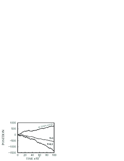
Figure 4: The position of the Brownian particle for the two temperatures, $T_{1}=1$ and $T_{2}=0.3$ and the alternating sequence $T_{1}T_{1}T_{2}T_{2}T_{1}T_{1}$. Just like in the games (Figure 2) we clearly see the inversion of [the direction of] movement when we alternate the two temperatures.

Let us see how to quantitatively study the energy exchange of this engine. In a certain step $t\rightarrow t+1$, in which the particle is in contact with, say, bath $1$, the energy transferred from the bath to the particle is

$$Q^{(1)}_{t\rightarrow t+1}=\sum^{\infty}_{x=-\infty}[\pi_{x}(t+1)-\pi_{x}(t)](V(x)+Fx)$$ (7)

where $\pi_{x}(t)$ is the probability that the particle is at the position $x$ in time $t$. The right hand side of the above equation can be decomposed into two terms

$$Q^{(1)}_{t\rightarrow t+1}=\triangle\mathcal{U}_{t\rightarrow t+1}-W_{t\rightarrow t+1}.$$ (8)

The first term is $\triangle\mathcal{U}_{t\rightarrow t+1}=\mathcal{U}_{t+1}-\mathcal{U}_{t}$, where $\mathcal{U}(t)$ is the internal energy of the system

$$\mathcal{U}(t)=\sum^{\infty}_{x=-\infty}\pi_{x}(t)V(x)=\langle V(x(t))\rangle.$$ (9)

On the other hand, the second term is the change of energy due to the external force $F$, that is, the work done by the force on the particle

$$W_{t\rightarrow t+1}=-F\langle v(t)\rangle$$ (10)

where $\langle{v}\rangle=\langle{x(t+1)}\rangle-\langle{x(t)}\rangle$ is the mean velocity of the particle. Hence Equation (10) has a simple interpretation: the work done by the force on the particle in a unit of time, or the power developed by the force, is the product of the force times the mean velocity of the particle. The minus sign arises because the direction of the force points to the left.

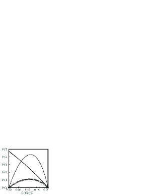
Figure 5: The efficiency $\eta$ of the thermal engine (continuous line), work $W$ done in each cycle (circles) and the current of particles (dotted line) as a function of the external force $F$ for $T_{1}=1$, $T_{2}=0.1$ and $V=1$.

The three quantities we have defined, the internal energy, heat and work are related through Equation (8), which is nothing else that the First Law of Thermodynamics (the sign convention we follow is the usual one in physics, namely, that heat and work are both positive if there is energy entering the system).

The same procedure is applied to the time-steps when the system is in contact with bath $2$. When we alternate the two baths in a cycle of four steps, $T_{1}T_{1}T_{2}T_{2}\ldots$, the system, after a certain number of cycles, reaches a regime where the internal energy and the mean velocity are periodic in time. In this regime we can compute the amount of heat extracted from each bath and the total work done by the force. The analytical treatment is analogous to the one carried out for the games and it is based on a three-state Markov chain. We shall not include here the details of the calculations but shall give some of the results that can be obtained. Applying equation (7) to the first two steps of the cycle we compute the energy $Q_{1}$ transferred from bath $1$ to the system, which is positive if $T_{1}>T_{2}$. However, when we apply the same equation to the last two steps of the cycle we obtain a negative energy $Q_{2}$, and, if $F$ is weak enough, we obtain a negative $W=-Q_{1}-Q_{2}$. These results tell us that the system extracts energy from the hot bath, dissipates part of this energy towards the cold bath and uses what remains of it to do work against the external force. The efficiency of the thermal engine is

$$\eta=-\frac{W}{Q_{1}}=1+\frac{Q_{2}}{Q_{1}}$$ (11)

which is positive and less than 1.

In Figure 5 we plot the engine efficiency as a function of the external force $F$. When the force is zero the efficiency is zero because the engine does not do any work and there is an irreversible heat transfer from the hot source to the cold one. Note that this holds even though in this case there exists a current of particles. For sufficiently strong forces the efficiency is once again zero. The reason is that the particles cannot move against strong forces. On the other hand, there exists a force for which the particle is, on the average, at rest and does not do work, while there still exists heat transfer from the hot bath to the cold one.

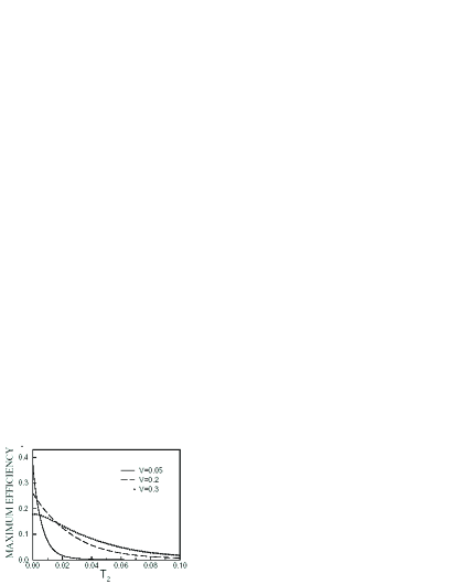
Figure 6: Efficiency of the thermal engine as a funtion of the temperature of the cold source $T_{2}$, for $T_{1}=1$ and several values of $V$. For each point, we have taken the value of the external force that maximizes the efficiency.

As it can be seen, the engine always works irreversibly, so it can never attain the efficiency of the Carnot engine. This is a common fact in the majority of Brownian motors [5, 7] (an exception are the reversible ratchets [8], whose efficiencies can be arbitrarily close to Carnot’s [7]), including the Feynman ratchet [9]. It is worth pointing out here that Feynman did not notice the intrinsic irreversibility of his thermal engine and went on to show that under a certain hypothesis that the engine could attain the Carnot efficiency. It has recently been shown that such hypotheses are incorrect [10].

In Figure 6 we show the engine’s efficiency for several temperatures $T_{2}$ keeping fixed the temperature $T_{1}$. Observe that the Carnot efficiency curve, $1-\frac{T_{2}}{T_{1}}=1-T_{2}$, is well above all the curves plotted in Figure 6.

4 Conclusions

We have shown a physical application of the paradoxical games, namely, in Brownian or molecular motors. The name “molecular motor” comes from biophysics where several forms of energy conversion within the cell are studied. For example, there are“pumps” capable of transporting ions from one side of a biological membrane to the other against the ion’s electrochemical gradient [11, 12]; molecules travelling through microtubules transporting diverse cellular material; or molecules capable of “pulling off” a filament and making up the muscular tissue [12]. Each one of these systems consists of a unique protein that changes its tri-dimensional configuration upon hydrolysis of ATP molecules. The protein is different for each system considered (kinesins in the transport through micro-channels, myosines in the muscular tissue), but all of them are motors capable of extracting the stored energy in the ATP bonds and transform it into mechanical energy. All these transformations are carried out at a scale where the thermal fluctuations are unavoidable.

For all this, we believe that in order to understand the energy-exchange processes at the cellular level a disposal of the authentic thermodynamics of Brownian motors will be essential. This thermodynamics will have to be, as we have seen, one of irreversible processes wherein the thermal fluctuations play a relevant role. It will, also, have to be different from the so-called finite-time thermodynamics, since the latter studies irreversible motors but of macroscopic character.

In recent years, the first steps have been taken towards building up the theory of molecular motors. Nevertheless, despite some work that shows general properties [7, 8, 10, 13, 14] most of the results so far refer to concrete models [4, 5] that are too simple to represent the behaviour of molecular motors.

Finally, we would like to conclude by recalling that the paradoxical games may have applications in other contexts. The paradox shows that the result of alternating two stochastic dynamics is far from being the “sum” or combination of the effects of each dynamic considered alone, and that could, in fact, be completely unexpected. This result should raise the interest in alternating dynamics in physical, biological and economics systems.

Appendix 1 – Markov Chain

A Markov chain is a set of $N$ states and we consider a particle that jumps in from one state to another in a probabilistic way and in discrete time steps. The Markov chain is defined by the matrix

$$\Pi=\{p_{i\rightarrow j}\}^{N}_{i,j=1}$$ (12)

where $p(i\rightarrow j)$ is the particle transition probability from state $i$ to the state $j$. Contrary to the usual matrix notation we shall use $i$ as the column index and $j$ as the row index. It can be readily checked that all the matrix elements are real numbers between $0$ and $1$ and that the entries of every column add up to $1$.

Let us call $\pi_{i}(t)$ the probability that the particle is in the state $i$ in time $t$. The probability to find the particle in the state $i$ at time $t+1$ is equal to the probability that the particle jumps, in the step $t\rightarrow t+1$, from any other state $j$ (including the case $i=j$), that is

$$\pi_{i}(t+1)=\sum^{N}_{j=1}\pi_{j}(t)p_{j\rightarrow i}.$$ (13)

Hence the distribution of probability $\pi(t)=(\pi_{1}(t),\ldots\pi_{N}(t))$ satisfies the following evolution equation

$$\vec{\pi}(t+1)=\Pi\vec{\pi}(t).$$ (14)

The distribution $\pi(t)$ tends, at large $t$, to a stationary distribution, $\pi^{\mathrm{st}}_{i}$, that satisfies equation (15)

$$\vec{\pi}^{\mathrm{st}}(t+1)=\Pi\vec{\pi}^{\mathrm{st}}(t)$$ (15)

that is, $\pi^{\mathrm{st}}$ is the eigenvector of the matrix $\Pi$ with eigenvalue $1$.

The stationary distribution tells us, in the limit of long times, what are the probabilities of the particle being in the different states $i=1,2,\ldots N$.

Game B consists of a Markov chain of three states, namely, $0$, $1$ and $2$. The matrix $\Pi$ is

$$\Pi=\left(\begin{array}[]{ccc}0&1-p_{2}&p_{2}\\ p_{3}&0&1-p_{2}\\ 1-p_{3}&p_{2}&0\\ \end{array}\right).$$ (16)

Notice that the elements of every column add up to $1$. The stationary probability distribution is

$$\vec{\pi}^{\mathrm{st}}=\frac{1}{Z}\left(1,\frac{p_{2}p_{3}+1-p_{2}}{1-p_{2}+p^{2}_{2}},\frac{p_{2}p_{3}+1-p_{3}}{1-p_{2}+p^{2}_{2}}\right)$$ (17)

where $Z$ is a normalization constant. Finally, a similar analysis holds for the random combination of games A and B upon substituting $p_{2}$ for $\frac{(p_{2}+p_{1})}{2}$ and $p_{3}$ for $\frac{(p_{3}+p_{1})}{2}$. From this stationary probability distribution $\pi^{\mathrm{st}}_{i}$ it is easy to compute the probability of winning in a particular run, as we have done in the main text.

Appendix 2 – The Metropolis algorithm

Let us suppose we have a physical system that can be in any of the states $i=1,2,\ldots N$ with energy $E_{i}$. What are the transition probabilities $p(i\rightarrow j)$ that govern the probabilistic evolution of the system when this is in contact with with a thermal bath at temperature $T$?

The requirement these transition probabilities have to satisfy is that they should eventually attain the Boltzmann distribution, that is, its stationary distribution should be

$$\vec{\pi}^{\mathrm{st}}=\frac{1}{Z}e^{-\beta E_{i}/kT}$$ (18)

where $Z$ is a normalized constant and $\beta=\frac{1}{kT}$, with $k$ the Boltzmann constant. Consequently, the transition matrix $\Pi$ has to be such that it has the distribution $\pi^{\mathrm{st}}$, given by (18), as its eigenvector with eigenvalue $1$.

A particular case is when the transition probabilities satisfy the condition of detailed balance

$$\pi^{\mathrm{st}}_{i}p_{i\rightarrow j}=\pi^{\mathrm{st}}_{j}p_{j\rightarrow i}.$$ (19)

An even more particular case is the Metropolis algorithm wherein the transition probabilities are given by the following rule, for $i\neq j$: or $i$ and $j$ are not connected, in which case $p(i\rightarrow j)=p(j\rightarrow i)=0$, or they are connected, so that

$$p_{i\rightarrow j}=\left\{\begin{array}[]{cc}\frac{1}{C_{i}}&\mathrm{if}\hskip 4.26773ptE_{j}\leq E_{i},\\ \frac{1}{C_{i}}e^{-(E_{j}-E_{i})\beta}&\mathrm{if}\hskip 4.26773ptE_{j}\geq E_{i},\end{array}\right.$$ (20)

where $C_{i}$ is chosen so that all the transition probabilities are between $0$ and $1$ (it often is the coordination number, i.e. the number of states connected to the state $i$) Finally, the transition probability from $i$ to itself is

$$p_{i\rightarrow i}=1-\sum_{j\neq i}p_{i\rightarrow j}$$ (21)

where the sum is carried over all the states $j$ connected to $i$. It can readily be checked that the transition probabilities so defined satisfy the condition of detailed balance.

We shall use the Metropolis algorithm in this article to model a particle in contact with a thermal bath. Notice also that in Equation (20) there is a non-zero probability that the particle increases its energy. These transitions are the result of thermal fluctuations where the thermal bath gives energy to the particle.

References

- [1] Harmer G.P. and Abbott D., “Parrondo’s paradox,” Statistical Science 14, 206-213 (1999); Harmer G.P. and Abbott D., “Losing strategies can win by Parrondo’s paradox,” Nature, 402, p. 864 (1999).
- [2] Harmer G.P., Abbott D., Taylor P.G. and Parrondo J.M.R., “Parrondo’s paradoxical games and the discrete Brownian ratchet,” In Proceedings of the 2nd International Conference on Unsolved Problems of Noise and Fluctuations, Eds. Abbott D. and Kiss L.B., 511, 189–200. American Institute of Physics (2000).
- [3] Karlin S. and Taylor H.M., A First Course in Stochastic Processes (Academic Press, New York, 1975).
- [4] Astumian R.D. and Bier M., “Fluctuation driven ratchets: molecular motors,” Phys. Rev. Lett., 72, 1766-1769 (1994).
- [5] Sokolov I.M. and Blumen A., “Non-equilibrium directed diffusion and inherently irreversible heat engines,” J. Phys. A, 30, 3021-3027 (1997).
- [6] Koonin S.E., Computational Physics (Benjamin/Cumings Publishing Inc., Menlo Park, California, 1975) Section 8.3.
- [7] Parrondo J.M.R., Blanco J.M., Cao F. and Brito R., “Efficiency of Brownian motors,” Europhys. Lett., 43, 248-254 (1998).
- [8] Parrondo J.M.R., “Reversible ratchets as Brownian particles in an adiabatically changing periodic potential,” Phys. Rev. E, 57, 7297-7300 (1998).
- [9] Feynman R.P., Leighton R.B. and Sands M., The Feynman Lectures on Physics (Addison- Wesley, Reading, Masachussetts, 1963), Vol. 1, pp. 46.1-46.9.
- [10] Parrondo J.M.R. and Español P., “Criticism of Feynman’s analysis of the ratchet as an engine,” Am. J. Phys., 64, 1125-1130 (1996).
- [11] Alberts B., Bray D., Lewis J., Raff M., Roberts K. and Watson J.D., Molecular Biology of The Cell (Garland Publishing Inc., New York, 1994) Chapters 11 and 14.
- [12] Cooper G.M., The Cell: A Molecular Approach, (Sinauer, Sunderland, Massachussets, 1997), Chapter 11.
- [13] Leibler S. and Huse D.A., “Porters versus rowers: a unified stochastic model of motor proteins,” J. of Cell Biol., 121, 1357-1368 (1993).
- [14] Magnasco M.O., “Molecular combustion motors,” Phys. Rev. Lett., 72, 2656 (1994).