The Origin of Magnetic Interactions in Ca₃Co₂O₆

Abstract

We investigate the microscopic origin of the ferromagnetic and antiferromagnetic spin exchange couplings in the quasi one-dimensional cobalt compound Ca₃Co₂O₆. In particular, we establish a local model which stabilizes a ferromagnetic alignment of the $S=2$ spins on the cobalt sites with trigonal prismatic symmetry, for a sufficiently strong Hund’s rule coupling on the cobalt ions. The exchange is mediated through a $S=0$ cobalt ion at the octahedral sites of the chain structure. We present a strong coupling evaluation of the Heisenberg coupling between the $S=2$ Co spins on a separate chain. The chains are coupled antiferromagnetically through super-superexchange via short O-O bonds.

Recently there has been renewed interest in systems exhibiting magnetization steps. In classical systems such as CsCoBr₃ one single plateau is typically observed in the magnetization versus field curve at one third of the magnetization at saturation.Hida94 This phenomenon attracted considerable attention, and Oshikawa, Yamanaka and Affleck demonstrated that Heisenberg antiferromagnetic chains exhibit such magnetization plateaus when embedded in a magnetic field.Oshikawa97 These steps are expected when $N_{c}(S-m)$ is an integer, where $N_{c}$ is the number of sites in the magnetic unit cell, $S$ the spin quantum number, and $m$ the average magnetization per spin, which we shall refer to as the OYA criterion. The steps can be stable when chains are coupled, for instance in a ladder geometry. In that case the magnetic frustration is an important ingredient to their stability.Mila98 Plateaus according to the OYA criterion are also anticipated for general configurations, provided gapless excitations do not destabilize them.Oshikawa00 Indeed several systems exhibiting magnetization steps are now known;Shiramura98 ; Narumi98 they all obey the OYA criterion, they are usually far from exhausting all the possible $m$ values, they all are frustrated systems, and they all can be described by an antiferromagnetic Heisenberg model. Related behavior has been recently found in other systems. For example, up to five plateaus in the magnetization vs. field curve have been observed in Ca₃Co₂O₆ at low temperatureAasland97 ; Kageyama97 ; Maignan00 . However there is to date no microscopic explanation to this phenomenon, even though the location of the plateaus is in agreement with the OYA criterion.

Ca₃Co₂O₆ belongs to the wide family of compounds A’₃ABO₆, and its structure belongs to the space group R3̄c. It consists of infinite chains formed by alternating face sharing AO₆ trigonal prisms and BO₆ octahedra — where Co atoms occupy both A and B sites. Each chain is surrounded by six chains separated by Ca atoms. As a result a Co ion has two neighboring Co ions on the same chain, at a distance of $2.59$ Å, and twelve Co neighbors on the neighboring chains at distances $7.53$ Å  (cf. Fig. 3).Fjellvag96 Concerning the magnetic structure, the experiment points toward a ferromagnetic ordering of the magnetic Co ions along the chains, together with antiferromagnetic correlations in the buckling a-b plane.Aasland97 The transition into the ordered state is reflected by a cusp-like singularity in the specific heat at 25 K,Hardy03 — at the temperature where a strong increase of the magnetic susceptibility is observed. Here we note that it is particularly intriguing to find magnetization steps in a system where the dominant interaction is ferromagnetic.

In order to determine the effective magnetic Hamiltonian of a particular compound one typically uses the Kanamori-Goodenough-Anderson (KGA) rulesGoodenough . Knowledge of the ionic configuration of each ion allows to estimate the various magnetic couplings. When applying this program to Ca₃Co₂O₆ one faces a series of difficulties specifically when one tries to reconcile the neutron scattering measurements that each second Co ion is non-magnetic. Even the assumption that every other Co ion is in a high spin state does not settle the intricacies related to the magnetic properties; one still has to challenge issues such as: i) what are the ionization degrees of the Co ions? ii) how is an electron transfered from one cobalt ion to a second? iii) which of the magnetic Co ions are magnetically coupled? iv) which mechanism generates a ferromagnetic coupling along the chains?

These questions are only partially resolved by ab initio calculations. In particular, one obtains that both Co ions are in 3+ configurations.Whangbo03 Moreover both Co-O and direct Co-Co hybridizations are unusually large, and low spin and high spin configurations for the Co ions along the chains alternate.Eyert03

Our publication addresses the magnetic couplings, and in particular the microscopic origin of the ferromagnetic coupling of two Co ions through a non-magnetic Co ion. In view of the plethoric variety of iso-structural compounds,Stitzer01 the presented mechanism is expected to apply to many of these systems. We now derive the magnetic inter-Co coupling for Ca₃Co₂O₆ from microscopic considerations. The high-spin low-spin scenario confronts us with the question of how a ferromagnetic coupling can establish itself, taking into account that the high spin Co ions are separated by over 5 Å, linked via a non-magnetic Co and several oxygens.

Let us first focus on the Co-atoms in a single Co-O chain of Ca₃Co₂O₆. As mentioned above the surrounding oxygens form two different environments in an alternating pattern. We denote the Co ion in the center of the oxygen-octahedron Co1, and the Co ion in the trigonal prisms Co2. The variation in the oxygen-environment leads to three important effects. First, there is a difference in the strength of the crystal field splitting, being larger in the octahedral environment. As a result Co1 is in the low spin state and Co2 in the high spin state. Second, the local energy levels are in a different sequence. For the octahedral environment we find the familiar $t_{2g}$–$e_{g}$ splitting, provided the axes of the local reference frame point towards the surrounding oxygens. The trigonal prismatic environment accounts for a different set of energy levels. For this local symmetry one expects a level scheme with $d_{3z^{2}-r^{2}}$ as lowest level, followed by two twofold degenerate pairs $d_{xy}$, $d_{x^{2}-y^{2}}$ and $d_{xz}$, $d_{yz}$. However, our LDA calculationsEyert03 show that the $d_{3z^{2}-r^{2}}$ level is actually slightly above the first pair of levels. Having clarified the sequence of the energy levels, we now turn to the microscopic processes which link the Co ions. Two mechanisms may be competing: either the coupling involves the intermediate oxygens, or direct Co-Co overlap is more important. Relying on electronic structure calculations, we may safely assume that the direct Co-Co overlap dominates.Eyert03 The identification of the contributing orbitals is more involved. Following Slater and KosterSlater54 one finds that only the $3z^{2}$-$r^{2}$ orbitals along the chains have significant overlap. However, we still have to relate the Koster-Slater coefficients and the coefficients for the rotated frame since the natural reference frames for Co1 and Co2 differ. On the Co2 atoms with the triangular prismatic environment the $z$-axis is clearly defined along the chain direction, and we choose the $x$ direction to point toward one oxygen. This defines a reference frame $S$. The $x$ and $y$ directions are arbitrary and irrelevant to our considerations. The octahedral environment surrounding the Co1 atoms defines the natural coordinate system, which we call $S^{\prime}$. By rotating $S^{\prime}$ onto $S$ one obtains the $3z^{2}$-$r^{2}$ orbital in the reference frame $S$ as an equally weighted sum of $x^{\prime}y^{\prime}$, $x^{\prime}z^{\prime}$, $y^{\prime}z^{\prime}$ orbitals in $S^{\prime}$. The above observation that the only significant overlap is due to the $3z^{2}$-$r^{2}$ orbitals on both Co ions now translates into an overlap of the $3z^{2}$-$r^{2}$ orbital on high spin cobalt with all $t_{2g}$ orbitals on low spin cobalt.

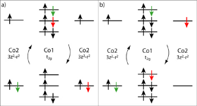
Figure 1: Typical hopping paths for a) ferromagnetic and b) antiferromagnetic ordering. The displayed ferromagnetic path is the only one for ferromagnetic ordering and has the highest multiplicity of all, ferromagnetic and antiferromagnetic. There are similar paths for antiferromagnetic ordering but with a Hund’s rule penalty and lower multiplicity. The path in (b) is unique for the antiferromagnetic case and has low energy but also low multiplicity.

We proceed with a strong coupling expansion to identify the magnetic coupling along the chain. This amounts to determine the difference in energy, between the ferromagnetic and antiferromagnetic configurations, to fourth order in the hopping, since this is the leading order to the magnetic interaction between the high spin Co ions. As explained above we only have to take into account the $3z^{2}$-$r^{2}$ level on Co2 and the $t_{2g}$ levels on Co1. In an ionic picture all $t_{2g}$ levels on Co1 are filled while the $d_{3z^{2}-r^{2}}$ level on Co2 is half-filled and we therefore consider hopping processes from the former to the latter. In the ferromagnetic configuration we include processes where two down spin electrons hop from Co1 to both neighboring Co2 and back again as displayed in Fig. 1a. There are in total $3\times 2\times 2\times 2\times 2=48$ such processes. The intermediate spin state for Co1 is in agreement with Hund’s rule. The energy gain per path is given by:

$${E_{f}=\frac{t^{4}}{E_{0}^{2}}\;\left(3U-5J_{\rm{H}}+4E_{\rm loc}(\Delta_{\rm{cf}},J_{\rm{H}},-1)\right)^{-1}}$$ (1)

with

$${E_{0}=U-J_{\rm{H}}+2E_{\rm loc}(\Delta_{\rm{cf}},J_{\rm{H}},-2)}$$ (2)

$$\Delta_{\rm{cf}}=\Delta_{\rm{Co1}}+\frac{4}{10}\Delta_{\rm{Co2}}$$ (3)

and

$${E_{\rm loc}(\Delta_{\rm{cf}},J_{\rm{H}},l)}={\frac{\Delta_{\rm{cf}}J_{\rm{H}}^{2}}{(\Delta_{\rm{cf}}-\frac{1}{2}lJ_{\rm{H}})(2\Delta_{\rm{cf}}+3J_{\rm{H}})}}$$ (4)

where $\Delta_{\rm{Co1}}$ and $\Delta_{\rm{Co2}}$ denote the crystal field splittings on Co1 and Co2, respectively. The Hund’s coupling is $J_{\rm{H}}$, assumed to be identical on both, Co1 and Co2, and $U$ denotes the local Coulomb repulsion. There are no further paths in this configuration, besides the one which twice iterates second order processes. In the antiferromagnetic case the situation is slightly more involved. Here three different classes of paths have to be distinguished. The first class, denoted $a1$ in the following, consists of hopping events of one up spin and one down spin electron from the same Co1 level. (There are $3\times 2\times 2=12$ such paths). The second class ($a2$) consists of hopping events of one down spin and one up spin electron from different Co1 levels (There are $3\times 2\times 2\times 2=24$ such paths). The third class ($a3$), shown in Fig. 1b, consists of hopping processes where one electron is hopping from Co1 to Co2 and then another electron is hopping from the other Co2 to the same Co1 and back again (There are $3\times 2=6$ such paths). In total this sums up to 42 paths in the antiferromagnetic configuration. Consequently, we have more ferromagnetic than antiferromagnetic exchange paths. However the energy gain depends on the path. For the classes $a1$ and $a2$, the intermediate Co1 state violates the Hund’s rule, and we identify an energy gain per path given by:

$$E_{a1} = \frac{t^{4}}{E_{0}^{2}}\left(3U-5J_{\rm{H}}+(4-\frac{6J_{\rm{H}}}{\Delta_{\rm{cf}}})E_{\rm loc}(\Delta_{\rm{cf}},J_{\rm{H}},1)\right)^{-1}$$

$$E_{a2} = \frac{t^{4}}{E_{0}^{2}}\left(3U-2J_{\rm{H}}-\rm{F}(\Delta_{\rm{cf}},J_{\rm{H}})\right)^{-1}$$ (5)

Here F is a positive function which is smaller than $J_{\rm{H}}$. The expression $3U-2J_{\rm{H}}-F$ is the lowest eigenvalue of $\langle i|H_{\rm Co}|j\rangle$ where the states $i$ and $j$ are all possible states on Co1 consistent with two of the $d$-orbitals filled and three empty. For the class $a3$ one observes that one does not need to invoke a Co1 ion with four electrons as an intermediate state, in contrast to all other processes we considered so far. We find the energy gain as:

$$E_{a3}=\frac{t^{4}}{E_{0}^{2}\left(U+2J_{\rm H}\right)}\\$$ (6)

Altogether we obtain the difference in energy gain between the ferromagnetic and the antiferromagnetic configurations as:

$$E^{\rm F}-E^{\rm AF}=48E_{f}-24E_{a1}-12E_{a2}-6E_{a3}$$ (7)

The dependence of $E^{\rm F}-E^{\rm AF}$ on $J_{\rm H}$ for different values of the local interaction $U$ is shown in Fig. 2. Using $J_{\rm H}=0.6~{}\rm{eV}$,Laschinger03 $U=5.3~{}\rm{eV}$,Sawatzky91 $t=1.5~{}\rm{eV}$,Eyert03 $\Delta_{\rm{Co1}}=2.5~{}\rm{eV}$ and $\Delta_{\rm{Co2}}=1.5~{}\rm{eV}$,Eyert03 we obtain an estimate for the Heisenberg exchange coupling (for the Co2 spin $S=2$):

$$J^{\rm F}=(E^{\rm F}-E^{\rm AF})/2S^{2}\approx 2\rm{meV}$$ (8)

which is in reasonable agreement with the experimental transition temperature of 25 K.

In this context one should realize that a one-dimensional chain does not support a true phase transition into the magnetic state. However, as the length $L$ of the chains is finite, a crossover into the ferromagnetic state may be observed when the correlation length is approximately $L$.chain

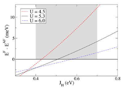
Figure 2: Energy gain $E^{\rm F}-E^{\rm AF}$ of a nearest neighbor Co2 ferromagnetic alignment with respect to an antiferromagnetic orientation as a function of the Hund’s coupling $J_{\rm H}$, for a typical parameter set of Hubbard $U$. The grey shaded area indicates the interval of $J_{\rm H}$ for which a Co2-high-spin Co1-low-spin configuration can be stabilized for the considered crystal field splittings.Laschinger03

To emphasize the importance of the chain geometry we now briefly discuss the hypothetical case where the $z$-axis of the octahedra corresponds to that of the prism. In this geometry there is only one orbital on each Co ion which contributes to the hopping processes. In this situation the process favoring ferromagnetism shown in Fig. 1a does not exist, in contrast to the process $a3$ shown in Fig. 1b, and the resulting coupling is therefore antiferromagnetic.

In the large class of known isostructural compoundsStitzer01 the non-magnetic ion is not necessarily a Co ion. If the non-magnetic ion is in a $3d^{2}$ (or $4d^{2}$) configuration, the above argument applies, and the coupling is antiferromagnetic. If the configuration is $3d^{4}$, all the discussed electronic processes contribute, however with different multiplicities. Moreover, additional paths have to be considered for the antiferromagnetic case. They represent exchange processes through an empty orbital on the non-magnetic ion. As a result, the ferromagnetic scenario has fewer paths than the antiferromagnetic, and the coupling becomes antiferromagnetic. Correspondingly, a ferromagnetic interaction can only occur when all three orbitals on the nonmagnetic ion participate in the exchange process. Obviously the situation we consider differs from the standard 180 degree superexchange mechanism in many respects.

With the investigation of the interchain magnetic interaction one first notices that each magnetic Co ion has twelve neighboring Co ions on different chains. However, as displayed in Fig. 3, there is an oxygen bridge to only six neighbors, one per chain. Here the coupling $J^{\rm AF}$ results from the super-superexchange mechanism (with exchange via two oxygen sites), and it is antiferromagnetic. Since the Co-O hybridization is unusally large in this system, we expect the interchain magnetic coupling to be sufficiently strong to account for the observed antiferromagnetic correlations.

From our previous considerations we introduce the minimal magnetic Hamiltonian:

$$H = \sum_{i,j}\left(J^{\rm F}_{i,j}{\vec{S}}_{i}\cdot{\vec{S}}_{j}+J^{\rm AF}_{i,j}{\vec{S}}_{i}\cdot{\vec{S}}_{j}\right)-D\sum_{i}S_{z,i}^{2}$$ (9)

$${\rm with} J^{\rm F}_{i,j}=\left\{\begin{array}[]{ll}J^{\rm F}&\mbox{if ${\vec{j}}-\vec{i}=\pm 2{\vec{d}}$}\\ 0&\mbox{otherwise}\end{array}\right.$$ (12)

$${\rm and}$$

$$J^{\rm AF}_{i,j}\! = \!\!\left\{\begin{array}[]{ll}J^{\rm AF}&\mbox{if ${\vec{j}}-\vec{i}=\pm({\vec{a}}+{\vec{d}}),\pm({\vec{b}}+{\vec{d}}),\pm({\vec{c}}+{\vec{d}})$}\\ 0&\mbox{otherwise.}\end{array}\right.$$ (14)

Here we use the site vectors ${\vec{a}}=a(-1/2,\sqrt{3}/2,c/(12a))$, ${\vec{b}}=a(-1/2,-\sqrt{3}/2,c/(12a))$, ${\vec{c}}=a(1,0,c/(12a))$, and ${\vec{d}}={\vec{a}}+{\vec{b}}+{\vec{c}}$ where $a=9.06$ Å and $c=10.37$ Å are the lattice constants of the hexagonal unit cell. The Hamiltonian, Eq. (9), also includes a phenomenological contribution $DS_{z}^{2}$ which accounts for the anisotropy observed, for example, in the magnetic susceptibility.Kageyama97a ; Maignan00

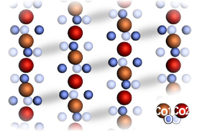
Figure 3: Projection of Ca₃Co₂O₆ in the (100) plane, with those oxygen atoms which are closest to the plane. Shadows indicate the shortest O-O bonds, along which super-superexchange processes take place. Yellow (red) large spheres denote Co1 (Co2) atoms, dark (light) small blue spheres oxygen atoms located above (below) the Co plane.

The stability of the magnetization steps results from the magnetic frustration which is introduced through the antiferromagnetic interchain coupling. Indeed, the lattice structure suggests that this magnetic system is highly frustrated, since the chains are arranged on a triangular lattice. However investigating the Hamiltonian (9) reveals that the microscopic mechanism leading to frustration is more complex. It is visualized when we consider a closed path $TLRT^{\prime}T$ — where the sites $T$ and $T^{\prime}$ are next nearest-neighbor Co2 sites on the same chain and the sequence of sites $TLR$ is located on a triangle of nearest neighbor chains. One advances from $T$ to $L$ to $R$ to $T^{\prime}$ on a helical pathcomment formed by the oxygen bridges from Fig. 3. Since the structure imposes $T$ and $T^{\prime}$ to be next nearest-neighbors, the frustration occurs independently of the sign of the intrachain coupling.

In summary we established the magnetic interactions in an effective magnetic Hamiltonian for Ca₃Co₂O₆. It is a spin-2 Hamiltonian, with antiferromagnetic interchain coupling, and ferromagnetic intrachain interactions. The latter is obtained from the evaluation of all spin exchange paths between two high-spin Co2 sites through an intermediary low-spin Co1 site. This mechanism is particular to the geometry of the system as is the microscopic mechanism which leads to magnetic frustration. We expect that the discussed microscopic mechanisms also apply to other isostructural compounds, such as Ca₃CoRhO₆ and Ca₃CoIrO₆.

- (1) F. Hida, J. Phys. Soc. Jpn. 63, 2359 (1994).
- (2) M. Oshikawa et al., Phys. Rev. Lett. 78, 1984 (1997).
- (3) F. Mila, Eur. Phys. J. B 6, 201 (1998).
- (4) M. Oshikawa, Phys. Rev. Lett. 84, 1535 (2000).
- (5) Y. Narumi et al., Physica B 246-247, 509 (1998).
- (6) W. Shiramura et al., J. Phys. Soc. Jpn. 67, 1548 (1998).
- (7) S. Aasland et al., Solid State Commun. 101, 187 (1997).
- (8) H. Kageyama et al., J. Phys. Soc. Jpn. 66, 1607 (1997).
- (9) A. Maignan et al., Eur. Phys. J. B 15, 657 (2000).
- (10) H. Fjellvåg et al., J. Sol. State Chem. 124, 190 (1996).
- (11) V. Hardy et al., Phys. Rev. B 68, 014424 (2003).
- (12) J. B. Goodenough, Magnetism and the Chemical Bond (Interscience Publishers, John Wiley & and sons, New York, 1963)
- (13) M. H. Whangbo et al., Solid State Commun. 125, 413 (2003).
- (14) V. Eyert et al., Preprint, unpublished (2003).
- (15) K. E. Stitzer et al., Opin. Solid State Mater. Sci. 5, 535 (2001).
- (16) J. C. Slater and G. F. Koster, Phys. Rev. 94, 1498 (1954).
- (17) C. Laschinger et al., J. Magn. and Magnetic Materials, (in press, 2004).
- (18) J. van Elp et al., Phys. Rev. B 44, 6090 (1991).
- (19) Given the strong magnetic anisotropy of Ca3Co2O6,Maignan00 which is phenomenologically included in Eq. (9), we expect that one can capture some physics of the system in the Ising limit. In that case, for a typical chain length of the order of one hundred sites, the correlation length extends to the system size for which is to be interpreted as the crossover temperature to the ferromagnetic state. Correspondingly, the spin susceptibility peaks at about which we verified in exact diagonalization. Even with chain lengths of 10,000 Co sites, the crossover temperature is still in the given range.
- (20) H. Kageyama et al., J. Phys. Soc. Jpn. 66, 3996 (1997).
- (21) The positions of the considered sites are: is an arbitrary Co2 site on any chain, , and .