Resonance Kondo Tunneling through a Double Quantum Dot at Finite Bias

Abstract

It is shown that the resonance Kondo tunneling through a double quantum dot (DQD) with even occupation and singlet ground state may arise at a strong bias, which compensates the energy of singlet/triplet excitation. Using the renormalization group technique we derive scaling equations and calculate the differential conductance as a function of an auxiliary dc-bias for parallel DQD described by $SO(4)$ symmetry. We analyze the decoherence effects associated with the triplet/singlet relaxation in DQD and discuss the shape of differential conductance line as a function of dc-bias and temperature.

I Introduction

Many fascinating collective effects, which exist in strongly correlated electron systems (metallic compounds containing transition and rare-earth elements) may be observed also in artificial nanosize devices (quantum wells, quantum dots, etc). Moreover, fabricated nanoobjects provide unique possibility to create such conditions for observation of many-particle phenomena, which by no means may be reached in ”natural” conditions. Kondo effect (KE) is one of such phenomena. It was found theoretically Glazr88b ; Ng88 and observed experimentally Gogo99 ; Cron98 ; Simmel99 that the charge-spin separation in low-energy excitation spectrum of quantum dots under strong Coulomb blockade manifests itself as a resonance Kondo-type tunneling through a dot with odd electron occupation ${\cal N}$ (one unpaired spin $S=1/2$). This resonance tunneling through a quantum dot connecting two metallic reservoirs (leads) is an analog of resonance spin scattering in metals with magnetic impurities. A Kondo-type tunneling arises under conditions which do not exist in conventional metallic compounds. The KE emerges as a dynamical phenomenon in strong time dependent electric field Goldin -Lopez01 , it may arise at finite frequency under light illumination Kex ; Shab00 ; Fujii01 . Even the net zero spin of isolated quantum dot (even ${\cal N}$) is not an obstacle for the resonance Kondo tunneling. In this case it may be observed in double quantum dots (DQD) arranged in parallel geometry KA02 , in T-shaped DQD KA01 ; KA02 ; Taka , in two-level single dots Izum ; Hoft or induced by strong magnetic field Magn ; Eto00 ; Giul01 ; Pust00 whereas in conventional metals magnetic field only suppresses the Kondo scattering. The latter effect was also discovered experimentally Sasa ; Nyg00 ; Wiel02 .

One of the most challenging options in Kondo physics of quantum dots is the possibility of controlling the Kondo effect by creating the non-equilibrium reservoir of fermionic excitations by means of strong bias $eV\gg T_{K}$ applied between the leads Meir ($T_{K}$ is the equilibrium Kondo temperature which determines the energy scale of low-energy spin excitations in a quantum dot). However, in this case the decoherence effects may prevent the formation of a full scale Kondo resonance (see, e.g. discussion in Refs. RKW, ; neq, ; Col, ). It was argued in recent disputes that the processes, associated with the finite current through a dot with odd ${\cal N}$ may destroy the coherence on an energy scale $\Gamma\gg T_{K}$ and thus prevent formation of a ground state Kondo singlet, so that only the weak coupling Kondo regime is possible in strongly non-equilibrium conditions.

In the present paper we discuss Kondo tunneling through DQD with even ${\cal N}$, whose ground state is a spin singlet $|S\rangle$. It will be shown that the Kondo tunneling through excited triplet state $|T\rangle$ arises at finite $eV$. In this case the ground state is stable against any kind of spin-flip processes induced by external current, the decoherence effects develop only in the intermediate (virtual) triplet state, and the estimates of decoherence rate should be revisited.

As was noticed in Ref. KA01, , quantum dots with even ${\cal N}$ possess the dynamical symmetry $SO(4)$ of spin rotator in the Kondo tunneling regime, provided the low-energy part of excitation spectrum is formed by a singlet-triplet (ST) pair, and all other excitations are separated from the ST manifold by a gap noticeably exceeding the tunneling rate $\gamma$. A DQD with even ${\cal N}$ in a side-bound (T-shape) configuration where two wells are coupled by the tunneling $v$ and only one of them (say, $l$) is coupled to metallic leads $(L,R)$ is a simplest system satisfying this condition KA01 . Such system was realized experimentally in Ref.mol95, . Novel features introduced by the dynamical symmetry in Kondo tunneling are connected with the fact that unlike the case of conventional $SU(2)$ symmetry of spin vector ${\bf S}$, the $SO(4)$ group possesses two generators ${\bf S}$ and ${\bf P}$. The latter vector describes transitions between singlet and triplet states of spin manifold (this vector is an analog of Runge-Lenz vector describing the hidden symmetry of hydrogen atom). As was shown in Ref. KA02, , this vector alone is responsible for Kondo tunneling through quantum dot with even ${\cal N}$ induced by external magnetic field.

Another manifestation of dynamical symmetry peculiar to DQDs with even ${\cal N}$ is revealed in this paper. It is shown that in the case when the ground state is singlet $|S\rangle$ and the S/T gap $\delta\gg T_{K}$, a Kondo resonance channel arises under a strong bias $eV$ comparable with $\delta.$ The channel opens at $|eV-\delta|<T_{K}$, and the tunneling is determined by the non-diagonal component $J_{ST}=\langle T|J|S\rangle$ of effective exchange induced by the electron tunneling through DQD (see Fig. 1 (right panel)).

II Cotunneling Hamiltonian of T-shaped DQD

The basic properties of symmetric DQD occupied by even number of electrons ${\cal N}=2n$ under strong Coulomb blockade in each well are manifested already in the simplest case $n=1$, which is considered below. Such DQD is an artificial analog of a hydrogen molecule ${\rm H_{2}}$. If the inter-well Coulomb blockade $Q$ is strong enough, one has ${\cal N}=n_{l}+n_{r},$ $n_{l}=n_{r}=1,$ the lowest states of DQD are singlet and triplet and the next levels are separated from ST pair by a charge transfer gap $\sim Q$. We assume that both wells are neutral at $n_{l,r}=1$. Then the effective inter-well exchange $I$ responsible for the singlet-triplet splitting arises because of tunneling $v$ between two wells, $I=v^{2}/Q=\delta$. It is convenient to write the effective spin Hamiltonian of isolated DQD in the form

$$H_{d}=E_{S}|S\rangle\langle S|+\sum_{\eta}E_{T}|T\eta\rangle\langle T\eta|\equiv\sum_{\Lambda=S,T\eta}E_{\Lambda}X^{\Lambda\Lambda}$$ (1)

where $X^{\Lambda\Lambda^{\prime}}=|\Lambda\rangle\langle\Lambda^{\prime}|$ is a Hubbard configuration change operator (see, e.g., Hewson ), $E_{T}=E_{S}+\delta$, $\eta=\pm,0$ are three projections of $S=1$ vector. Two other terms completing the Anderson Hamiltonian, which describes the system shown in Fig.1 (left panel), are

$$H_{b}+H_{t}=$$

$$\sum_{k\alpha\sigma}\epsilon_{k\alpha}c^{\dagger}_{k\alpha\sigma}c_{k\alpha\sigma}+\sum_{\Lambda\lambda}\sum_{k\alpha\sigma}\left(W^{\Lambda\lambda}_{\sigma}c_{k\alpha\sigma}^{\dagger}X^{\lambda\Lambda}+H.c.\right).$$ (2)

The first term describes metallic electrons in the leads and the second one stands for tunneling between the leads and the DQD. Here $\alpha=L,R$ marks electrons in the left and right lead, respectively, the bias $eV$ is applied to the left lead, so that the chemical potentials are $\mu_{FL}=\mu_{FR}+eV$,  $W^{\Lambda\lambda}_{\sigma}$ is the tunneling amplitude for the well $l$ (left), $|\lambda\rangle$ are one-electron states of DQD, which arises after escape of an electron with spin projection $\sigma$ from DQD in a state $|\Lambda\rangle$.

Figure 1: Left panel: Double quantum dot in a side-bound configuration. Right panel: cotunneling processes in biased DQD responsible for the resonance Kondo tunneling.

We solve the problem in a Schrieffer-Wolff (SW) limit Hewson , when the activation energies $|E_{\Lambda}-E_{\lambda}-\mu_{F\alpha}|$ and Coulomb blockade energy $Q$ are essentially larger then the tunneling rate $\gamma$, and charge fluctuations are completely suppressed both in the ground and excited state of DQD. In this limit one may start with the SW transformation, which projects out charge excitations. We confine ourselves with the bias $eV\lesssim\delta\ll D$, where $D$ is the width of the electrons in the leads, so the leads are considered in the SW transformation as two independent quasi equilibrium reservoirs (cf. Goldin ; Kam00 ). As is shown in Ref. KA01 , the SW transformation being applied to a spin rotator results in the following effective spin Hamiltonian

$$H_{int}=\sum_{\alpha\alpha^{\prime}}[(J^{TT}_{\alpha\alpha^{\prime}}{\bf S}+J^{ST}_{\alpha\alpha^{\prime}}{\bf P})\cdot{\bf s}_{\alpha\alpha^{\prime}}+J^{SS}_{\alpha\alpha^{\prime}}X^{SS}n_{\alpha\alpha^{\prime}}]$$ (3)

Here ${\bf s}_{\alpha\alpha^{\prime}}$$=$$\sum_{kk^{\prime}}c^{\dagger}_{k\alpha\sigma}\hat{\tau}c_{k^{\prime}\alpha^{\prime}\sigma^{\prime}}$,  $n_{\alpha\alpha^{\prime}}$$=$$\sum_{kk^{\prime}}c^{\dagger}_{k\alpha\sigma}\hat{1}c_{k^{\prime}\alpha^{\prime}\sigma}$, $\hat{\tau}$,  $\hat{1}$ are the Pauli matrices and unity matrix respectively. The effective exchange constants are

$$J^{\Lambda\Lambda^{\prime}}_{\alpha\alpha^{\prime}}\approx\frac{W^{\Lambda\lambda}_{\sigma}W^{*\lambda\Lambda^{\prime}}_{\sigma}}{2}\left(\frac{1}{\epsilon_{F\alpha}-E_{S}/2}+\frac{1}{\epsilon_{F\alpha^{\prime}}-E_{S}/2}\right).$$

In this approximation the small differences between singlet and triplet states are neglected. Besides, $J_{\alpha\alpha^{\prime}}^{\Lambda\Lambda^{\prime}}\sim I$ in real DQD.

Two vectors ${\bf S}$ and ${\bf P}$ with spherical components

$$S^{+}=\sqrt{2}\left(X^{10}+X^{0-1}\right),~{}S^{-}=\sqrt{2}\left(X^{01}+X^{-10}\right),$$

$$S_{z}=X^{11}-X^{-1-1},\,\;\;\;P_{z}=-\left(X^{0S}+X^{S0}\right),$$

$$P^{+}=\sqrt{2}\left(X^{1S}-X^{S-1}\right),P^{-}=\sqrt{2}\left(X^{S1}-X^{-1S}\right).$$ (4)

obey the commutation relations of $o_{4}$ algebra

$$[S_{j},S_{k}]=ie_{jkl}S_{l},~{}[P_{j},P_{k}]=ie_{jkl}S_{l},~{}[P_{j},S_{k}]=ie_{jkl}P_{l}$$

($j,k,l$ are Cartesian coordinates, $e_{jkl}$ is a Levi-Civita tensor). These vectors are orthogonal, ${\bf S\cdot P}=0,$ and the Casimir operator is ${\bf S}^{2}+{\bf P}^{2}=3.$ Thus, the singlet state is involved in spin scattering via the components of the vector ${\bf P}$.

We use $SU(2)$-like semi-fermionic representation for $S$ operators popov ; kis00

$$S^{+}=\sqrt{2}(f_{0}^{\dagger}f_{-1}+f^{\dagger}_{1}f_{0}),\;\;\;S^{-}=\sqrt{2}(f^{\dagger}_{-1}f_{0}+f_{0}^{\dagger}f_{1}),$$

$$S_{z}=f^{\dagger}_{1}f_{1}-f^{\dagger}_{-1}f_{-1},$$ (5)

where $f^{\dagger}_{\pm 1}$ are creation operators for fermions with spin “up” and “down” respectively, whereas $f_{0}$ stands for spinless fermion popov ; kis00 . This representation can be generalized for $SO(4)$ group by introducing another spinless fermion $f_{s}$ to take into consideration the singlet state. As a result, the $P$-operators are given by the following equations:

$$P^{+}=\sqrt{2}(f^{\dagger}_{1}f_{s}-f_{s}^{\dagger}f_{-1}),\;\;\;P^{-}=\sqrt{2}(f_{s}^{\dagger}f_{1}-f^{\dagger}_{-1}f_{s}),$$

$$P^{z}=-(f_{0}^{\dagger}f_{s}+f_{s}^{\dagger}f_{0}).$$ (6)

The Casimir operator ${\bf S}^{2}+{\bf P}^{2}=3$ transforms to the local constraint

$$\sum_{\Lambda=\pm,0,s}f^{\dagger}_{\Lambda}f_{\Lambda}=1.$$

The final form of the spin cotunneling Hamiltonian is

$$H_{int}=\sum_{kk^{\prime},\alpha\alpha^{\prime}=L,R}J^{S}_{\alpha\alpha^{\prime}}f_{s}^{\dagger}f_{s}c^{\dagger}_{k\alpha\sigma}c_{k^{\prime}\alpha^{\prime}\sigma}$$ (7)

$$+\sum_{kk^{\prime},\alpha\alpha^{\prime}\Lambda\Lambda^{\prime}}\left(J^{T}_{\alpha\alpha^{\prime}}\hat{S}^{d}_{\Lambda\Lambda^{\prime}}+J^{ST}_{\alpha\alpha^{\prime}}\hat{P}^{d}_{\Lambda\Lambda^{\prime}}\right)\tau^{d}_{\sigma\sigma^{\prime}}c^{\dagger}_{k\alpha\sigma}c_{k^{\prime}\alpha^{\prime}\sigma^{\prime}}f_{\Lambda}^{\dagger}f_{\Lambda^{\prime}}$$

where $\hat{S}^{d}$ and $\hat{P}^{d}$ ($d$$=$$x$,$y$,$z$) are $4\times 4$ matrices defined by relations (4) - (6) and $J^{S}=J^{SS}$, $J^{T}=J^{TT}$ and $J^{ST}$ are singlet, triplet and singlet-triplet coupling SW constants, respectively.

The cotunneling in the ground singlet state is described by the first term of the Hamiltonian (7), and no spin flip processes accompanying the electron transfer between the leads emerge in this state. However, the last term in (7) links the singlet ground state with the excited triplet and opens a Kondo channel. In equilibrium this channel is ineffective, because the incident electron should have the energy $\delta$ to be able to initiate spin-flip processes. We will show in the next section that the situation changes radically, when strong enough external bias is applied.

III Kondo singularity in tunneling through DQD at finite bias

We deal with the case, which was not met in the previous studies of non-equilibrium Kondo tunneling. The ground state of the system is singlet, and the Kondo tunneling in equilibrium is quenched at $T\sim\delta$. Thus, the elastic Kondo tunneling arises only provided $T_{K}\gg\delta$ in accordance with the theory of two-impurity Kondo effect KA01 ; Varma . However, the energy necessary for spin flip may be donated by external electric field $eV$ applied to the left lead, and in the opposite limit $T_{K}\ll\delta$ the elastic channel emerges at $eV\approx\delta$. The processes responsible for resonance Kondo cotunneling at finite bias are shown in Fig. 1 (left panel).

In conventional spin $S=1/2$ quantum dots the Kondo regime out of equilibrium is affected by spin relaxation and decoherence processes, which emerge at $eV\gg T_{K}$ (see, e.g., Kam00 ; RKW ; neq ; Col ). These processes appear in the same order as Kondo co-tunneling itself, and one should use the non-equilibrium perturbation theory (e.g., Keldysh technique) to take them into account in a proper way. In our case these effects are expected to be weaker, because the nonzero spin state is involved in Kondo tunneling only as an intermediate virtual state arising due to S/T transitions induced by the second term in the Hamiltonian (3), which contains vector ${\bf P}$. The non-equilibrium repopulation effects in DQD are weak as well (see next section, where the nonequilibrium effects are discussed in more details).

Having this in mind, we describe Kondo tunneling through DQD at finite $eV\lesssim\delta$ within the quasi-equilibrium perturbation theory in a weak coupling regime (cf. the quasi-equilibrium approach to description of decoherence rate at large $eV$ in Ref. RKW, ). To develop the perturbative approach for $T>T_{K}$ we introduce the temperature Green’s functions (GF) for electrons in a dot, ${\cal G}_{\Lambda}(\tau)=-\langle T_{\tau}f_{\Lambda}(\tau)f^{\dagger}_{\Lambda}(0)\rangle,$ and GF for the electrons in the left (L) and right (R) lead, $G_{L,R}(k,\tau)=-\langle T_{\tau}c_{L,R\sigma}(k,\tau)c^{\dagger}_{L,R\sigma}(k,0)\rangle$. Performing a Fourier transformation in imaginary time for bare GF’s, we come to following expressions:

$$G^{0}_{k\alpha}(\epsilon_{n})=(i\epsilon_{n}-\epsilon_{k\alpha}+\mu_{L,R})^{-1},$$

$${\cal G}^{0}_{\eta}(\omega_{m})=(i\omega_{m}-E_{T})^{-1},\;\;\;\eta=-1,0,1$$

$${\cal G}^{0}_{s}(\epsilon_{n})=(i\epsilon_{n}-E_{S})^{-1},$$ (8)

with $\epsilon_{n}=2\pi T(n+1/2)$ and $\omega_{m}=2\pi T(m+1/3)$ popov ; kis00 . The first leading and next to leading parquet diagrams are shown on Fig.2.

Figure 2: Leading (b,d) and next to leading (c,e) parquet diagrams determining renormalization of $J^{S}(a)$. Solid lines denote electrons in the leads. Dashed lines stand for electrons in the dot.

Corrections to the singlet vertex $\Gamma(\omega,0;\omega^{\prime},0)$ are calculated using an analytical continuation of GF’s to the real axis $\omega$ and taking into account the shift of the chemical potential in the left lead. Since the electron from the left lead tunnels into the empty state in the right lead separated by the energy $eV$, we have to put $\omega=eV$, $\omega^{\prime}=0$ in the final expression for $\Gamma(\omega,0;\omega^{\prime},0)$. Thus, unlike conventional Kondo effect we deal with the vertex at finite frequency $\omega$ similarly to the problem considered in Ref. RKW, . We assume that the leads remain in equilibrium under applied bias and neglect the relaxation processes in the leads (“hot” leads). In a weak coupling regime $T>T_{K}$ the leading non-Born contributions to the tunnel current are determined by the diagrams of Fig. 2 b-e.

The effective vertex shown in Fig. 2b is given by the following equation

$$\Gamma_{LR}^{(2b)}(\omega)=J_{LL}^{ST}J_{LR}^{TS}\sum_{\bf k}\frac{1-f(\epsilon_{kL}-eV)}{\omega-\epsilon_{kL}+\mu_{L}-\delta}$$ (9)

Changing the variable $\epsilon_{kL}$ for $\epsilon_{kL}-eV$ one finds that

$$\Gamma_{LR}^{(2b)}(\omega=eV)\sim J_{LL}^{ST}J_{LR}^{TS}\nu\ln(D/{\rm max}\{(eV-\delta),T\}).$$

Here $D\sim\varepsilon_{F}$ is a cutoff energy determining effective bandwidth, $\nu$ is a density of states on a Fermi level and $f(\varepsilon)$ is the Fermi function. Therefore, under condition $|eV-\delta|\ll\max[eV,\delta]$ this correction does not depend on $eV$ and becomes quasielastic.

Unlike the diagram Fig. 2b, its ”parquet counterpart” term Fig. 2c contains $eV+\delta$ in the argument of the Kondo logarithm:

$$\Gamma_{LR}^{(2c)}(\omega)=J_{LL}^{ST}J_{LR}^{TS}\sum_{\bf k}\frac{f(\epsilon_{kL}-eV)}{\omega-\epsilon_{kL}+\mu_{L}+\delta}$$ (10)

At $eV\sim\delta\gg T$ this contribution is estimated as

$$\Gamma_{LR}^{(2c)}(eV)\sim J_{LL}^{ST}J_{LR}^{TS}\nu\ln~{}(D/(eV+\delta))\ll\Gamma_{LR}^{(2b)}(eV).$$

Similar estimates for diagrams Fig.2d and 2e give

$$\Gamma_{LR}^{(2d)}(\omega)\sim J_{LL}^{ST}J_{LL}^{T}J_{LR}^{TS}\nu^{2}\ln^{2}~{}(D/{\rm max}\{\omega,(eV-\delta),T\})$$

$$\Gamma_{LR}^{(2e)}(\omega)\sim J_{LL}^{ST}J_{LL}^{T}J_{LR}^{TS}\nu^{2}\ln~{}(D/{\rm max}\{\omega,(eV-\delta),T\})\times$$

$$\times\ln~{}(D/{\rm max}\{\omega,eV,T\}.$$ (11)

Then $\Gamma_{LR}^{(2e)}(\omega)\ll\Gamma_{LR}^{(2d)}(\omega)$ at $eV\to\delta$.

Thus, the Kondo singularity is restored in non-equilibrium conditions where the electrons in the left lead acquire additional energy in external electric field, which compensates the energy loss $\delta$ in a singlet-triplet excitation. The leading sequence of most divergent diagrams degenerates in this case from a parquet to a ladder series.

Following the poor man’s scaling approach, we derive the system of coupled renormalization group (RG) equations for (7). The equations for LL co-tunneling are:

$$\frac{dJ^{T}_{LL}}{d\ln D}=-\nu(J_{LL}^{T})^{2},\;\;\;\frac{dJ^{ST}_{LL}}{d\ln D}=-\nu J_{LL}^{ST}J_{LL}^{T},$$ (12)

The scaling equations for $J_{LR}^{\Lambda}$ are as follows:

$$\frac{dJ^{T}_{LR}}{d\ln D}=-\nu J_{LL}^{T}J_{LR}^{T},\;\;\;\frac{dJ^{ST}_{LR}}{d\ln D}=-\nu J_{LL}^{ST}J_{LR}^{T},$$

$$\frac{dJ^{S}_{LR}}{d\ln D}=\frac{1}{2}\nu\left(J_{LL,+}^{ST}J_{LR,-}^{TS}+\frac{1}{2}J_{LL,z}^{ST}J_{LR,z}^{TS}\right).$$ (13)

One-loop diagrams corresponding to the poor man’s scaling procedure are shown in Fig. 3. To derive these equations we collected only terms $\sim(J^{T})^{n}\ln^{n+1}(D/T)$ neglecting contributions containing $\ln[D/(eV)]$. The analysis of RG equations beyond the one loop approximation will be published elsewhere.

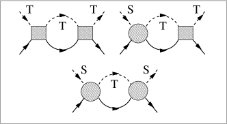
Figure 3: Irreducible diagrams contributing to RG equations. Hatched boxes and circles stand for triplet-triplet and singlet-triplet vertices respectively. Notations for lines are the same as in Fig.2

The solution of the system (13) reads as follows:

$$J^{T}_{\alpha,\alpha^{\prime}}=\frac{J^{T}_{0}}{1-\nu J^{T}_{0}\ln(D/T)},\;\;\;J^{ST}_{\alpha,\alpha^{\prime}}=\frac{J^{ST}_{0}}{1-\nu J^{T}_{0}\ln(D/T)},$$

$$J^{S}_{LR}=J^{S}_{0}-\frac{3}{4}\nu(J^{ST}_{0})^{2}\frac{\ln(D/T)}{1-\nu J^{T}_{0}\ln(D/T)}.$$ (14)

Here $\alpha=L$, $\alpha^{\prime}=L,R$. One should note that the Kondo temperature is determined by triplet-triplet processes only in spite of the fact that the ground state is singlet. One finds from (14) that $T_{K}=D\exp[-1/(\nu J^{T}_{0})]$. This temperature is noticeably smaller than the ”equilibrium” Kondo temperature $T_{K0}$, which emerges in tunneling through triplet channel in the ground state, namely $T_{K}\approx T_{K0}^{2}/D$. The reason for this difference is the reduction of usual parquet equations for $T_{K}$ to a simple ladder series. In this respect our case differs also from conventional Kondo effect at strong bias RKW , where the non-equilibrium Kondo temperature $T^{*}\approx T_{K0}^{2}/eV$ arises. In our model the finite bias does not enter $T_{K}$ because of the compensation $eV\approx\delta$ in spite of the fact that we take the argument $\omega=eV$ in the vertex (9).

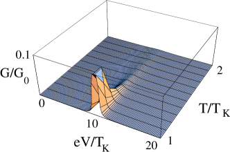
Figure 4: The Kondo conductance as a function of dc-bias $eV/T_{K}$ and $T/T_{K}$. The singlet-triplet splitting $\delta/T_{K}=10$.

The differential conductance $G(eV,T)/G_{0}\sim|J^{ST}_{LR}|^{2}$ (cf. Ref. KNG, ) is the universal function of two parameters $T/T_{K}$ and $eV/T_{K}$,  $G_{0}=e^{2}/\pi\hbar$:

$$G/G_{0}\sim\ln^{-2}\left(\max[(eV-\delta),T]/T_{K}\right)$$ (15)

Its behavior as a function of bias and temperature is shown in Fig. 4. It is seen from this picture that the resonance tunneling ”flashes” at $eV\sim\delta$ and dies away out of this resonance. In this picture the decoherence effects are not taken into account, and it stability against various non-equilibrium corrections should be checked.

IV Decoherence effects

We analyze now the decoherence rate $\hbar/\tau_{d}$ associated with T/S transition relaxation induced by cotunneling. The calculations are performed in the same order of the perturbation theory as it has been done for the vertex renormalization (see Figs. 2 and 3). The details of the calculation scheme are presented in Appendix.

To estimate the decoherence effects, one should calculate the decay of the triplet state or in other terms to find the imaginary part of the retarded self energy of triplet semi-fermion propagators at actual frequency [see discussion before Eq. (9)], $\hbar/\tau_{d}=-2{\rm Im}\Sigma^{R}_{T}(\omega)$. The 2nd and 3rd order diagrams determining $\hbar/\tau_{d}$ are shown in Fig.5(a-d). Two leading terms given by the diagrams of Fig.5(a,b) describe the damping of triplet excitation due to its inelastic relaxation to the ground singlet state. These terms are calculated in Appendix (see Eqs. (A.8), (A.10)). One finds from these equations that the relaxation rate associated with ST transition is

$$1/\tau_{d}^{ST}\sim\left(J^{ST}/D\right)^{2}{\rm max}[eV,\omega,T_{K}].$$ (16)

It should be noted that for corrections associated with LL (RR) diagrams (Fig.5a), describing co-tunneling processes on a left (right) lead, the use of quasi-equilibrium technique is fully justified when the leads themselves are in thermal equilibrium. We are interested in the zero frequency damping at resonance $eV\approx\delta$. Neglecting the small difference between $J^{T}$ and $J^{ST}$ (see KA01 ), we also take $J^{T}\approx J^{ST}=J$. Thus the $T\to S$ spin relaxation effect (16) does not contain logarithmic enhancement factor in the lowest order. It is estimated as

$$1/\tau_{d}^{ST}\sim(eV)\cdot(J/D)^{2}\approx J^{3}/D^{2}~{}.$$ (17)

The repolulation of triplet state as a function of external bias is controlled by the occupation number for triplet state modified by the bias $eV$. The latter, in turn, depends on the modified exchange splitting $\delta^{*}$ given by solution of the equation

$$\delta^{*}-\delta=Re\Sigma^{R}(\delta^{*},eV,T).$$ (18)

The $Re\Sigma^{R}$ (Fig.5(a,b)) is given by

$$Re\Sigma^{R(2)}_{TST}(\omega,eV,T)=-a_{2}\left(\frac{J}{D}\right)^{2}\omega\ln\left(\frac{D}{{\rm max}[\omega,eV,T]}\right)$$ (19)

where $a_{2}\sim 1$ is a numerical coefficient. As it is seen, the perturbative equation for $Re\Sigma^{R}$ is beyond the scope of leading-log approximation. As a result, $\delta^{*}(eV)-\delta\ll\delta$ and repopulation of the triplet state is exponentially small. The corresponding factor in the occupation number is

$$P_{t}(eV)=\exp\left(-\delta^{*}(eV)/T\right)$$ (20)

The effects of repopulation become important only at $eV\gg\delta$ when $|\delta^{*}-\delta|\sim\delta$. In that case the quasi equilibrium approach is not applicable and one should start with the Keldysh formalism RKW ; neq . This regime is definitely not realized in conditions considered above.

Next 2nd order contribution is the damping of triplet state itself given by Eqs. (A.12), (A.14). It is seen from these equations that this damping is of threshold character:

$$1/\tau_{d}^{TT}\sim(J/D)^{2}(\omega-\delta)\theta(\omega-\delta)~{},$$ (21)

where $\theta(\omega)$ is a Heaviside step function. These processes emerge only at $\omega>\delta$, so unlike the conventional case RKW they are not dangerous.

Corresponding contribution to $Re\Sigma^{R}$ casts the form

$$Re\Sigma^{R(2)}_{TTT}=-b_{2}\left(\frac{J}{D}\right)^{2}(\delta-\omega)\ln\left|\frac{D}{{\rm max}[(\delta-\omega),T]}\right|,$$ (22)

where $b_{2}\sim 1$.

Figure 5: Leading diagrams (a-d) for $\hbar/\tau_{d}$ (see text). Dashed line in the self-energy part stands for the singlet state of a two-electron configuration in the dot.

Next, one have to check whether the higher order logarithmic corrections modify the estimate (17). These corrections start with the 3-rd order terms shown in Fig. 5(c,d). Straightforward calculations lead to $eV(J/D)^{3}\ln(D/eV)$ correction (see the first term Eq. A.23). This leading term like the 2-nd order term originates from $T\to S$ spin relaxation processes. All other contributions are either of threshold character, or vanish at $\omega\to 0$. As a result, the estimate

$$\hbar/\tau_{d}\sim eV(J^{ST}_{0}/D)^{2}[1+O(\nu J\ln(D/(eV))]$$

holds. The topological structure (sequence of intermediate singlet and triplet states and cotunneling processes in the left and right lead) in perturbative corrections for the triplet self energy part is different from those for the singlet-singlet vertex (see Appendix). Namely, the leading (ladder) diagrams for the vertex contain maximal possible number of intermediate triplet states, whereas the higher order non-threshold log-diagrams for the self energy part must contain at least one intermediate singlet state. As it is seen from the Appendix (Eq.(A.18)-(A.23)), the higher order contributions to $Im\Sigma_{T}(\omega)$ are not universal and the coefficients in front of log have sophisticated frequency dependence. As a result, the perturbative series for triplet self-energy part can not be collected in parquet structures and remain beyond the leading-log approximation discussed in the Section III. There is no strong enhancement of the 2nd order term in $SO(4)$ spin rotator model in contrast to $SU(2)$ case discussed in RKW . As was pointed out above, the main reason for differences in estimates of coherence rate is that in case of QD with odd ${\cal N}$, the Kondo singlet develops in the ground state of the dot, and decoherence frustrate this ground state. In DQD with even ${\cal N}$ the triplet spin state arises only as a virtual state in cotunneling processes, and our calculations demonstrate explicitely that decoherence effects in this case are essentially weaker.

The 3-rd order correction to $Re\Sigma$ is given by

$$Re\Sigma^{R(3)}(\omega)\sim\left(\frac{J}{D}\right)^{3}\omega\ln^{2}\left(\frac{D}{\omega}\right)$$ (23)

(see Appendix). This correction also remains beyond the leading-log approximation.

Thus we conclude that the decoherence effects are not destructive for Kondo tunneling through T-shaped DQD, i.e. the $T_{K}\gg\hbar/\tau_{d}$ is valid provided

$$\delta(\delta/D)^{2}\ll T_{K}\ll\delta.$$ (24)

This interval is wide enough because $\delta/D\ll 1$ in the Anderson model.

The same calculation procedure may be repeated in Keldysh technique. It is seen immediately that in the leading-log approximation the off-diagonal terms in Keldysh matrix are not changed in comparison with equilibrium distribution functions because of the same threshold character of repopulation processes, so in the leading approximation the key diagram Fig. 5b (determining L-R current through the dot) calculated in Keldysh technique remains the same as (A.8)-(A.10).

In fact, repopulation effects result in asymmetry of the Kondo-peak similar to that in Ref. neq, due to the threshold character of ${\rm Im}\Sigma_{TTT}$ (see Appendix). This asymmetry becomes noticeable at $eV\gg\delta$, where our quasi equilibrium approach fails, but this region is beyond our interest, because the bias-induced Kondo tunneling is negligible at large biases (see Fig. 4).

V Concluding remarks

We have shown in this paper that the tunneling through DQD with even ${\cal N}$ with singlet ground state and triplet excitation divided by the energy gap $\delta\gg T_{K}$ from the singlet state exhibits a peak in differential conductance at $eV\approx\delta$ (Fig. 4). This result is in striking contrast with the zero bias anomaly (ZBA) at $eV\approx 0$ which arises in the opposite limit, $\delta<T_{K}$. In the latter case the Kondo screening is quenched at energies less than $\delta$, so the ZBA has a form of a dip in the Kondo peak (see Hoft for detailed explanation of this effect).

In this case strong external bias initiates the Kondo effect in DQD, whereas in a conventional situation (QD with odd ${\cal N}$ spin 1/2 in the ground state) strong enough bias is destructive for Kondo tunneling. We have shown that the principal features of Kondo effect in this specific situation may be captured within a quasi equilibrium approach. The scaling equations (13), (14) can also be derived in Schwinger-Keldysh formalism (see Refs. kis00, ; neq, ) by applying the “poor man’s scaling” approach directly to the dot conductance Goldin .

Of course, our RG approach is valid only in the weak coupling regime. Although in our case the limitations imposed by decoherence effects are more liberal than those existing in conventional QD, they apparently prevent the full formation of the Kondo resonance. To clarify this point one has to use a genuine non-equilibrium approach, and we hope to do it in forthcoming publications.

One should mention yet another possible experimental realization of resonance Kondo tunneling driven by external electric field. Applying the alternate field $V=V_{ac}\cos(\omega t)$ to the parallel DQD, one takes into consideration two effects, namely (i) enhancement of Kondo conductance by tuning the amplitude of ac-voltage to satisfy the condition $|eV_{ac}-\delta|\ll T_{K}$ and (ii) spin decoherence effects due to finite decoherence rate Goldin . One can expect that if the decoherence rate $\hbar/\tau\gg T_{K},$

$$G_{peak}/G_{0}\sim\ln^{-2}\left(\hbar/\tau T_{K}\right)$$ (25)

whereas in the opposite limit $\hbar/\tau\ll T_{K}$,

$$G_{peak}=\overline{G(V_{ac}\cos[\omega t])}$$ (26)

is averaged over a period of variation of ac bias. In this case the estimate (15) is also valid.

In conclusion, we have provided the first example of Kondo effect, which exists only in non-equilibrium conditions. It is driven by external electric field in tunneling through a quantum dot with even number of electrons, when the low-lying states are those of spin rotator. This is not too exotic situation because as a rule, a singlet ground state implies a triplet excitation. If the ST pair is separated by a gap from other excitons, then tuning the dc-bias in such a way that applied voltage compensates the energy of triplet excitation, one reaches the regime of Kondo peak in conductance. This theoretically predicted effect can be observed in dc- and ac-biased double quantum dots in parallel geometry.

References

- (1) L.I.Glazman and M.E.Raikh, JETP Lett.47, 452, (1988).
- (2) T.K.Ng and P.A.Lee, Phys.Rev.Lett.61, 1768 (1988).
- (3) D. Goldhaber-Gordon, J. Göres, M. A. Kastner, H. Shtrikman, D. Mahalu, and U. Meirav, Phys.Rev.Lett. 81, 5225 (1998).
- (4) S.M. Cronenwett, T.H. Oosterkamp, and L.P. Kouwenhoven, Science, 281, 540 (1998).
- (5) F. Simmel, R. H. Blick, J. P. Kotthaus, W. Wegscheider, and M. Bichler, Phys. Rev. Lett. 83, 804 (1999).
- (6) T.K. Ng, Phys. Rev. Lett. 76, 487 (1996).
- (7) M. H. Hettler, J. Kroha, and S. Hershfield, Phys. Rev. B58, 5649 (1998).
- (8) Y. Goldin and Y. Avishai, Phys. Rev. Lett. 81, 5394 (1998), Phys. Rev. B61, 16750 (2000).
- (9) A. Kaminski, Yu. V. Nazarov, and L. I. Glazman, Phys. Rev. B62, 8154 (2000);
- (10) R. López, R. Aguado, G. Platero, and C. Tejedor, Phys. Rev. B 64, 075319 (2001).
- (11) K. Kikoin and Y. Avishai, Phys. Rev. B62, 4647 (2000);
- (12) T. V. Shahbazyan, I. E. Perakis, and M. E. Raikh, Phys. Rev. Lett., 84, 5896 (2000).
- (13) T. Fujii and N. Kawakami, Phys. Rev. B63, 064414 (2001).
- (14) K.Kikoin and Y.Avishai, Phys. Rev. B65, 115329 (2002).
- (15) K.Kikoin and Y.Avishai, Phys. Rev. Lett. 86, 2090 (2001).
- (16) Y. Takazawa, Y. Imai and N. Kawakami, J. Phys. Soc. Jpn, 71, 2234 (2002).
- (17) W. Izumida, O. Sakai and Y. Shimizu, J. Phys. Soc. Jpn, 67 2444 (1998);
- (18) W.Hofstetter and H.Schoeller, Phys.Rev.Lett 88, 016803 (2002).
- (19) M. Pustilnik, Y. Avishai, and K. Kikoin, Phys. Rev. Lett. 84, 1756 (2000).
- (20) M. Eto and Yu. Nazarov, Phys. Rev. Lett. 85, 1306 (2000), Phys. Rev. B64, 085322 (2001).
- (21) D. Giuliano, B. Jouault, and A. Tagliacozzo, Phys. Rev. B63, 125318 (2001).
- (22) M. Pustilnik and L.I. Glazman, Phys. Rev. Lett. 85, 2993 (2000), Phys. Rev. B64, 045328 (2001).
- (23) S. Sasaki, S. De Franceschi, J. M. Elzerman, W. G. van der Wiel, M. Eto, S. Tarucha, L. P. Kouwenhoven, Nature 405, 764 (2000).
- (24) J. Nygård, D.H. Cobden, P.E. Lindelof, Nature 408, 342 (2000).
- (25) W. G. van der Wiel, S. De Franceschi, J. M. Elzerman, S. Tarucha, L. P. Kouwenhoven, J. Motohisa, F. Nakajima, and T. Fukui, Phys. Rev. Lett. 126803 (2002).
- (26) Y. Meir and N. S. Wingreen, Phys.Rev.Lett. 68, 2512 (1992), Phys.Rev. B49,11040 (1994).
- (27) A. Rosch, J. Kroha, and P. Wölfle, Phys. Rev. Lett., 87, 156802 (2001).
- (28) A.Rosch, J.Paaske, J.Kroha, and P.Wölfle, Phys. Rev. Lett. 90, 076804 (2003).
- (29) O.Parcollet and C.Hooley, Phys.Rev. B66, 085315 (2002), P.Coleman and W.Mao, cond-mat/0203001, cond-mat/0205004.
- (30) L. W. Molenkamp, K. Flensberg, and M. Kemerink, Phys. Rev. Lett. 75, 4282 (1995).
- (31) A.C. Hewson, The Kondo Problem to Heavy Fermions (Cambridge University Press, Cambridge, 1993).
- (32) V.N.Popov and S.A.Fedotov, Sov.Phys.JETP 67, 535 (1988).
- (33) M.N.Kiselev and R.Oppermann, Phys. Rev. Lett 85, 5631 (2000).
- (34) M.N.Kiselev, H.Feldmann, and R.Oppermann, Eur. Phys. J B22, 53 (2001).
- (35) B.A.Jones and C.M.Varma, Phys.Rev. B40, 324 (1989).
- (36) Possibility of additional Kondo peaks at in strong magnetic field was noticed also in papers of Ref. [18], [21].
- (37) A. Kaminski, Yu. V. Nazarov, and L. I. Glazman, Phys.Rev.Lett 83, 384 (1999).
- (38) A.Abrikosov, Physics 2, 21 (1965).
- (39) A.A.Abrikosov and A.A.Migdal, J.Low Temp. Phys. 5, 519 (1970).
- (40) M.Abramowitz and I.Stegun, Handbook of mathematical functiuons. (Dover Publications, New York, 1965).