Abstract

We introduce a population dynamics model, where individual ge- nomes are represented by bit-strings. Selection is described by death probabilities which depend on these genomes, and new individuals continuously replace the ones that die, keeping the population constant. An offspring has the same genome as its (randomly chosen) parent, except for a small amount of (also random) mutations. Chance may thus generate a newborn with a genome that is better than that of its parent, and the newborn will have a smaller death probability. When this happens, this individual is a would-be founder of a new lineage. A new lineage is considered created if its alive descendence grows above a certain previously defined threshold. The time evolution of populations evolving under these rules is followed by computer simulations and the probability densities of lineage duration and size, among others, are computed. These densities show a scale-free behaviour, in accordance with some conjectures in paleoevolution, and suggesting a simple mechanism as explanation for the ubiquity of these power-laws.

Keywords: Evolution, lineage branching, Monte Carlo simulations

1 Introduction

Biological evolution of species presents some universal behaviour due to its time-and-size scaleless character (see, for instance, [1]). A parallel between this feature and critical phenomena studied within statistical physics is straightforward, and indeed many techniques traditionally used by physicists in this field were recently adopted also to study evolution through simple computer models (see, for instance, [2]). Two of the most important lessons physicists have learnt from critical phenomena are listed below.

Lesson 1: One cannot take only a small piece (or a small time interval) of the system under study, including later the rest of the system as a perturbation. Critical, scale-free systems resist to this approach, because they are non-linear, the whole is not simply the sum of the parts. All scales of size (and time) are equally important for the behaviour of the whole system. A would-be upper bound for size (or lifetime), above which one can neglect the corresponding effects, does not exist.

Lesson 2: The specific microscopic (or short term) details of the system are not definitive to determine the behaviour of the whole system under a macroscopic (or long term) point of view. In other words, systems which are completely different in their microscopic constituents (or short term evolution rules) can present the same critical, macroscopic behaviour. In particular, some universal critical exponents determine a mathematical behaviour that is shared by completely distinct systems. Thus, one can indirectly study some aspects of a complicated real system by observing the evolution of an artificially invented toy model simulated on the computer.

There are many evidences for this scale-free behaviour within biological evolution. Among others, a famous example is the classification of extinct genera according to their lifetime, a long term study of fossil data performed by paleontologists John Sepkoski and David Raup [3, 4, 5]. The frequency distribution they found is compatible with a power-law decay with exponent 2. The same exponent was confirmed by at least two distinct theoretical computer models [6, 7].

Branching processes in general also show scale-free behaviour. In this case, an important class, with exponents multiple of $1/4$, is ubiquitous. This interesting issue was studied by G.B. West and collaborators, a recent overview can be found in [8]. In particular, by studying blood transport networks, they proposed a model based on three basic ingredients: a hierarchical branching pattern, where a vessel bifurcates into smaller vessels and so on; a minimum cut-off size for the smallest branches, which makes the branching mechanism a finite process; and a free-energy minimisation constraint. From these three basic hypotheses, they were able to show the emergence of the exponents $1/4,1/2,3/4$, etc [9, 10, 11]. Of course, not only blood vessel systems follow this general framework, and the same class of exponents multiple of $1/4$ were indeed measured within many other contexts.

A particularly intriguing example is the so-called Kleiber’s empirical law, discovered in 1932. It relates the metabolic energetic power $P$ of an animal (mammal) with its mass $M$ as $P\sim M^{3/4}$. The validity of this relation goes down to single isolated mammalian cells and even its isolated mitochondrian, covering 26 orders of magnitude [9]. Also, lifespan increases with $M^{1/4}$ for many organisms, while heart-rate decreases with $M^{-1/4}$. Thus, the number of heart-beats during the whole life is invariant for all mammals. Similar scaling relations and invariant quantities appear at the molecular level as well [9].

Here, we raise the idea that biological speciation could fit very well into the general branching process framework described by West. Why would the idea of universality apply to evolutionary systems is an interesting and important conceptual question. Some hints towards a possible answer can be seen in [12, 13, 14, 15].

In the present work, in order to test this possible link between biological speciation and West’s framework, we address such a complicated problem, namely lineage branching, following the quoted toy model approach. Our hope is that some of the quantities we can measure could have a parallel in the real world, in particular the critical exponents. Besides the computer simulations from which we measure these quantities and their related critical exponents, we were also able to relate them with each other. This further analytical treatment yields some scaling relations which are completely fullfilled by our simulational results. Furthermore, these relations allow us to predict the unknown values of some exponents from the knowledge of others, an approach which could be very useful since only one such exponent was directly measured by fossil data, namely from the Sepkoski and Raup work. First, we present the model, then the results of our computer simulations and analytical approaches. Conclusions are at the end.

2 The model

Our population is kept constant, with $P$ (typically $10^{5}$ or $10^{6}$) individuals representing a sample of a much larger set. Each individual is characterised only by its genome, represented here by an array of $g$ bits (typicaly 32, 64, 128 $\dots$ 2048). Each bit can either be set (1-bit) or not (0-bit). At the beginning, all bits are zeroed, and all individuals belong to a single lineage.

We count the total number $N_{i}$ of bits set along the genome of individual $i$: it will survive with probability $x^{N_{i}+1}$, which decreases exponentially for increasing values of $N_{i}$, i.e. the larger the number of 1-bits along the genome, the larger is the death probability of this particular individual. This is the selection ingredient of our model. At each time step, a certain fraction $b$ (typically 1% or 2%) of individuals die, each one according to its own death probability, as the outcome of intralineage competition.

At each time step, the simulation obtains the value of $x$ first, before the death cycle, by solving the polynomial equation

$$\sum_{i}\,x^{N_{i}+1}=P(1-b)\,\,\,\,\,\,\,\,,$$ (1)

where the sum runs over all living individuals. This requirement keeps the population constant. Equivalently, one can solve

$$\sum_{N}\,H(N)\,\,x^{N+1}=P(1-b)\,\,\,\,\,\,\,\,,$$ (2)

where now the sum runs over $N$ (0, 1, 2 $\dots$), and $H(N)$ counts the current number of individuals with precisely $N$ bits set along the genome. After computing the value of $x$, we scan the whole population ($i$ = 1, 2 $\dots P$), tossing a real random number between 0 and 1 for each individual $i$, in order to compare it with its survival probability: if the random number is larger than $x^{N_{i}+1}$, individual $i$ dies.

Figure 1: Number of living lineages, normalised by the population, as a function of time, for different genome lengths.

After each death, we choose another individual at random to be the parent of a newborn. Its genome is copied, and some random mutations are included at a fixed rate per bit (typically 1/32) which does not depend on the genome length. Each mutation flips the current bit state (from 0 to 1 or vice-versa) at a position tossed along the genome. After all mutations are performed, the newborn is included into the population.

Figure 2: Number of living lineages, normalised by the population, averaged over the final $10^{5}$ time steps of the simulation, as a function of the genome length.

If the newborn presents fewer 1-bits than its parent, it receives the label of potential founder of a new lineage. During the time steps that follow, all its descendents will be monitored: if, at some future time, the number of those descendents still alive reaches a minimum threshold $s_{0}$ (typically 10), then all descendents of the now confirmed founder, including itself, are considered to belong to a new lineage.

On the other hand, extinction occurs when the last individual of a given lineage dies. Although a rare event, a lineage can also become extinct if all its individuals descend from the same potential founder, being altogether transferred to another, new, lineage, by reaching the threshold $s_{0}$.

A similar model, but without the lineage branching step, was already used by some of us [16].

3 Results

We have run our program with some different sets of parameters $\{P$, $s_{0}$, $b\}$. The results are qualitatively the same in all cases, thus we will present only results for populations with $P=10^{5}$ individuals, $b=2\%$ of which die every year (immediately replaced by newborns), requiring a minimum threshold of $s_{0}=10$ living descendents of the same potential founder in order to have a new lineage. The genome lengths vary from $g=32$ up to $g=2048$. We have also studied an alternate version of the model in which, instead of being strictly constant, the population is allowed to fluctuate: first, all individuals have the chance to generate offspring, according to the rate $b$, increasing the population; after that, the death roulette kills individuals according to the probability $1-x^{N_{i}+1}$. No change is observed in what concerns the quantities we measured below. Also, similar branching criteria were introduced into the Penna model for biological ageing [17, 2], for smaller genome lengths $g=8$, 16, 32 and 64: the general behaviour did not change.

Figure 1 shows the number of living lineages as a function of time $t$. Each time step corresponds to a scan of the whole population performing deaths and births. We divided the number of living lineages by the constant number of individuals, in order to show that one lineage indeed corresponds to a considerable number of individuals (varying from approximately ten thousand, on average, for the largest genome length of 2048 bits, down to fifty individuals for the smallest genome length of 32 bits). One can also observe that the total number of generations we tested, after one million time steps, is large enough to get a stable, self-organised situation which is, indeed, very different from the starting point, with a single lineage and completely clean genomes.

Figure 3: Probability density distributions for $N/g$, where $N$ counts the number of 1-bits along a genome of length $g$.

Figure 4: Number of lineages which become extinct per “year” (one time step), averaged over intervals of $10^{3}$ time steps, as a function of time.

Figure 5: Total number of extinct lineages as a function of the genome length.

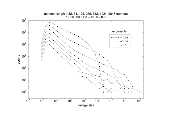
Figure 6: Distribution of extinct lineages according to size $s$ (total number of individuals which belonged to that lineage) for different genome lengths.

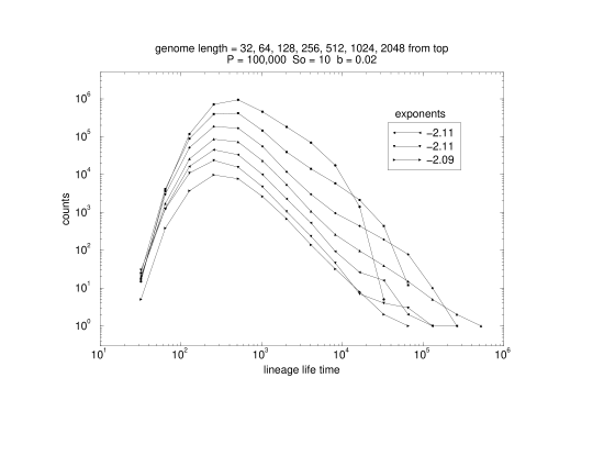
Figure 7: Distribution of extinct lineages according to lifetime $\ell$, for different genome lengths.

Over the last one hundred thousand time steps, after stabilisation, we have performed the average of the number of living lineages for each genome length. The results are displayed in figure 2. The exponent that figures in the plot was obtained from a fit to the simulation data. For other runs, with different sets of parameters, it remained the same. The relation between these two quantities (number $L$ of living lineages and genome length $g$) follows a power-law of the kind

$$L\,\propto\,g^{-\beta}\,\,\,\,,\,\,\,\,\,\,\,\,\beta\approx 5/4\,\,\,\,\,\,\,\,.$$ (3)

Here, we propose that the numerically determined value $\beta=1.24$ (error bar within the last digit) is in fact $\beta=5/4$, falling into the same family of simple multiples of 1/4, ubiquitous among biological measurements of various kinds (see [8, 9, 10, 11, 14, 18] and references therein). As already quoted, G. West and collaborators demonstrated the emergence of exponents multiple of $1/4$ based only on three fundamental ingredients. Our lineage model shares the same ingredients, namely:

1) a multiple hierarchical branching — in our case, lineages born from others;

2) a size invariant limit for the final branch — in our case, we require a fixed minimum population $s_{0}$ in order to have branching;

3) a free-energy minimisation process — in our case, the growing-entropy tendency provided by the random mutations (in the direction of randomising the bits along the genome as time goes by) is balanced by the selection mechanism (which gives preference to individuals with the smallest possible number of 1-bits).

Figure 3 illustrates this last ingredient. By counting the number of 1-bits along each genome, the results are distributed far below half of the whole length $g$ (which would be the maximum-entropy situation), showing the efficiency of the selection process. On the other hand, the non-vanishing width observed in the same distributions shows a high degree of genetic diversity preserved within the survivors, even when the genome length is varied. Note that, with the exception of the three smallest genome lengths (symbols), all other curves (small black dots) collapse into a single, genome-length-independent one, within the figure scale.

Figure 4 shows the number of lineages which become extinct each year, as a function of time. Extinction becomes more difficult for larger genome lengths. Figure 5 shows the total number $N$ of extinct lineages, during the whole one-million-time-step history, as a function of the genome length. Again, we observe a power-law behaviour according to the general trend

$$N\,\propto\,g^{-\gamma}\,\,\,\,,\,\,\,\,\,\,\,\,\gamma\approx 1\,\,\,\,\,\,\,\,.$$ (4)

Figure 6 shows the distributions of extinct lineages as a function of their sizes. One observes again a power-law behaviour with exponent very close to 1 (even for parameters other than the ones used for this particular plot). The exponents obtained from a fit to the data corresponding to the largest genome lengths are shown. The position of the peak does not change when the genome length is increased, in agreement with our criterion for branching, namely a fixed minimum number $s_{0}$ of living individuals. Thus, in the limit of large populations and large genome lengths, the probability distribution of lineages size $P(s)$ is expected to be

$$P(s) = C\,s^{-\lambda}\,\,\,\,\,\,\,\,{\rm if}\,\,\,\,s\geq s_{0},\,\,\,\,{\rm where}\,\,\,\,\lambda\approx 1$$

$$= 0\,\,\,\,\,\,\,\,{\rm otherwise}\,\,\,\,\,\,\,\,.$$

The value of $\lambda$ can be exactly 1 or slightly larger than 1, and the constant $C$ does not depend on the genome length.

The distribution of lineage lifetime, figure 7, is different. Its peak position does depend on the genome length $g$. At the same limit of large populations and large genome lengths, its probability ${\cal P}(\ell)$ reads

$${\cal P}(\ell) = (\alpha-1)\,\,[\ell_{0}(g)]^{\alpha-1}\,\,\ell^{-\alpha}\,\,\,\,\,\,\,\,{\rm if}\,\,\,\,\ell\geq\ell_{0}(g),\,\,\,\,\,{\rm where}\,\,\,\,\alpha\approx 2$$

$$= 0\,\,\,\,\,\,\,\,{\rm otherwise}\,\,\,\,\,\,\,\,.$$

Again, $\alpha$ can be exactly 2 or slightly larger than 2. This value is in complete agreement with the real exponent found by paleontologists John Sepkoski and David Raup from fossil data. The multiplicative constant in front of $\ell^{-\alpha}$ can be easily obtained by integrating equation (6) and equating the result to unity: for $\alpha=2$, it coincides with the minimum cutoff lifetime $\ell_{0}(g)$ itself.

The dependence of $\ell_{0}$ on $g$ also follows a power-law behaviour

$$\ell_{0}\,\propto\,g^{-\delta}\,\,\,\,,\,\,\,\,\,\,\,\,\delta\approx 1/4\,\,\,\,\,\,\,\,,$$ (7)

as can be seen, for instance, by plotting the peak positions on figure 7 against $g$. Alternatively, and with better accuracy, one can plot the average lifetime against $g$. The exponent we get from this plot (not shown) is 0.26, for our simulational data. Indeed, a simple reasoning can link the number $L(g)$ of living lineages at a given time, equation (3), with the number $N(g)$ of extinct lineages during the whole history, equation (4). The former can be counted by adding the probability of each lineage $j$ to be alive at a given time, i.e. its lifetime $\ell_{j}$ divided by the whole historical time $T$,

$$L(g)=\sum_{j=1}^{N(g)}{\ell_{j}\over T}={N(g)\over T}\int_{\ell_{0}}^{T}d\ell\,\,\ell\,\,{\cal P}(\ell)\,\,\,\,\,\,\,\,.$$ (8)

Considering $\ell_{0}<<T$, we get

$$L(g)\,\,\propto\,\,N(g)\,\,\ell_{0}(g)\,\,\,\,\,\,\,\,,$$ (9)

and the consequent scaling relation

$$\beta=\gamma+\delta$$ (10)

which holds in general (apart from small logarithmic corrections, if $\alpha=2$). This relation is very well verified by our numerical data.

The ratio 2:1 we found between the exponents $\alpha$ and $\lambda$ governing the two probability distributions for lineages (according to their lifetime or size) has an interesting interpretation. The growth of the number of lineages is not restricted by the finite size of the whole population. Each lineage grows by itself, reaches its maximum number of individuals, and then shrinks up to extinction due to its own genetic meltdown. If the maximum number of living individuals belonging to a lineage was somehow limited by an external source, then this maximum would be kept for a long time, waiting for the unavoidable genetic meltdown which eventually leads to extinction: in this case, the relation between lineage size $s$ and lifetime $\ell$ would be linear. On the contrary, we obtain a relation

$$s\,=\,A(g)\,\ell^{\omega}\,\,\,\,,\,\,\,\,\,\,\,\,\omega\approx 2\,\,\,\,,$$ (11)

in agreement with the ratio $\alpha/\lambda\approx 2$ we got previously from the lifetime and size distribution probabilities, separately. We have measured $\omega$ independently, by accumulating a $[\ell,s]$ histogram of all lineages, an example of which is shown in the table, for a genome length of 64. Lineages live in a narrow stripe of the space $[\ell,s]$, near the line defined by equation (11). For all genome lengths, $\omega$ is always very close to 2, according to our simulational data.

Table 1: Probability distribution of species as a function of lifetime $\ell$ and size $s$. Fractions smaller than 0.0001 are not shown.

1048576	.	.	.	.	.	.	.	.	.	.0001
524288	.	.	.	.	.	.	.	.	.0001	.0001
262144	.	.	.	.	.	.	.	.	.0006	.
131072	.	.	.	.	.	.	.	.0005	.0007	.
65536	.	.	.	.	.	.	.	.0018	.0002	.
32768	.	.	.	.	.	.	.0010	.0020	.	.
16384	.	.	.	.	.	.	.0035	.0007	.	.
8192	.	.	.	.	.	.0014	.0050	.	.	.
4096	.	.	.	.	.	.0066	.0026	.	.	.
2048	.	.	.	.	.0010	.0120	.0003	.	.	.
1024	.	.	.	.	.0090	.0102	.	.	.	.
512	.	.	.	.0003	.0253	.0039	.	.	.	.
256	.	.	.	.0109	.0425	.0008	.	.	.	.
128	.	.	.0005	.0692	.0372	.	.	.	.	.
64	.	.	.0323	.1705	.0140	.	.	.	.	.
32	.	.0105	.2210	.1190	.0008	.	.	.	.	.
16	.0021	.0644	.1007	.0050	.	.	.	.	.	.
8	.0015	.0047	.0007	.	.	.	.	.	.	.
$s/\ell$	64	128	256	512	1024	2048	4096	8192	$2^{14}$	$2^{15}$

By using the identity $P(s)ds={\cal P}(\ell)d\ell$, one can also show the further relation

$$s_{0}\sim A(g)\,\,[\ell_{0}(g)]^{\omega}\,\,\,\,,\,\,\,\,\,\,\,\,{\rm or}\,\,\,\,\,\,\,\,\ell_{0}(g)\,\,\propto\,\,[A(g)]^{-1/\omega}\,\,\,\,\,\,\,\,,$$ (12)

from which one can again (and independently) extract the exponent $\delta$ relating $\beta$ and $\gamma$, through the proportionality constants $A(g)$, equation (11), provided by the $[\ell,s]$-histograms.

4 Conclusions

We study a simple population dynamics model where the genome of each individual is represented by a bit-string. The survival probability decreases with the number of 1-bits along the individual’s genome. At each time step, a certain fraction of individuals die according to these probabilities, and are replaced by survival’s offspring. The genome of each offspring is a copy of the parent’s, with a few random mutations. Lineage branching occurs when an offspring happens to have a genome better than its parent, provided its own descendence succeeds in growing up to surpass a threshold of living individuals.

By simulating this simple model on a computer, we find some general power-law relations which seem to be independent of the particular parameters adopted in the simulations, and also of modifications of the dynamic rules themselves. One of these power-laws, namely equation (6) describing the distribution of extinct lineages per lifetime, agrees with real paleontological data [3, 4, 5], for which the exponent $\alpha\approx 2$ also agrees with our numerically determined value. No real data is available in order to compare the other exponents we measured (equations 3, 4, 5, 7 and 11). Nevertheless, we were also able to obtain some analytical scaling relations between these various exponents, all of them in agreement with our numerical data. Moreover, within our narrow error bars, all these exponents are multiple of $1/4$, in complete agreement with the general framework theoretically studied by West et al [9, 10, 11] in a different context. These authors show the emergence of exponents multiple of $1/4$, which are ubiquitous within biological systems, based only on three very general assumptions also shared by our model. Thus, we propose these exponents could be universal, valid for other evolutionary systems more complicated than our toy model.

References

- [1] S.A. Kauffman, Origins of Order: Self-Organization and Selection in Evolution, Oxford University Press, Oxford (1993).
- [2] S. Moss de Oliveira, P.M.C. de Oliveira and D. Stauffer, Evolution, Money, War and Computers: Non-Traditional Applications of Computational Statistical Physics, Teubner, Stuttgart/Leipzig (1999).
- [3] J.J. Sepkoski Jr., Paleobiology 19, 43 (1993).
- [4] D.M. Raup, Science 231, 1528 (1986).
- [5] D.M. Raup, Extinction: Bad Genes or Bad Luck, Norton, New York (1991).
- [6] M.E.J. Newman and B.W. Roberts, Proc. Royal Soc. B260, 31 (1995).
- [7] R.V. Solé and S.C. Manrubia, Phys. Rev. E54, R42 (1996)
- [8] V.M. Savage, J.F. Gillooly, W.H. Woodruff, G.B. West, A.P. Allen, B.J. Enquist and J.H. Brown, Functional Ecology 18, 257 (2004).
- [9] G.B. West, Physica A263, 104 (1999).
- [10] B.J. Enquist, J.H. Brown and G.B. West, Nature 395, 163 (1998).
- [11] G.B. West, J.H. Brown and B.J. Enquist, Science 276, 122 (1997).
- [12] M. Doebeli and G.D. Ruxton, Evolution 51, 1730 (1997).
- [13] S.A.H. Geritz, E. Kisdi, G. Meszéna and J.A. Mertz, Evo. Ecol. 12, 35 (1998).
- [14] G. Parisi, Physica A263, 557 (1999).
- [15] P.M.C. de Oliveira, COND-MAT 0101170, short version published in Theory in Biosciences 120, 1 (2001).
- [16] S. Moss de Oliveira, P.M.C. de Oliveira and D. Stauffer, Physica A322, 521 (2003) (COND-MAT 0208439).
- [17] T.J.P. Penna, J. Stat. Phys. 78, 1629 (1995).
- [18] L. Demetrius, Quantum Statistics, Allometric Relations in Biology and Evolutionary Dynamics, préprint (2003).