Two-Dimensional Diffusion in the Presence of Topological Disorder

Abstract

How topological defects affect the dynamics of particles hopping between lattice sites of a distorted, two-dimensional crystal is addressed. Perturbation theory and numerical simulations show that weak, short-ranged topological disorder leads to a finite reduction of the diffusion coefficient. Renormalization group theory and numerical simulations suggest that longer-ranged disorder, such as that from randomly placed dislocations or random disclinations with no net disclinicity, leads to subdiffusion at long times.

I Introduction

Diffusion in random media is a well-studied problem Bouchaud and Georges (1990). The mean-square displacement of a tracer particle behaves at long times in a way that depends on the character of the random forces induced on the tracer by the disorder. Forces that arise from random potentials lead to a reduction of the transport, with subdiffusion possible for diffusion of an ion in a medium with quenched charges obeying bulk charge neutrality Bouchaud and Georges (1990). Interestingly, the same subdiffusion results from diffusion of an ion in a medium with randomly-placed, quenched dipoles Nelson (1983); Rubinstein et al. (1983); Cha and Fertig (1995); Park and Deem (1998a). Forces that arise from entrainment along fluid streamlines lead to an increase in the transport, with the well-known result of turbulent super-diffusion possible for random streamlines with statistics characteristic of fluid turbulence Bouchaud and Georges (1990).

Distortion of the underlying lattice upon which the diffusion occurs is a very different type of disorder. In particular, topological defects such as dislocations or disclinations should affect the transport properties of a diffusing tracer particle. These topological defects cause a global rearrangement of the connectivity of the lattice upon which the diffusion occurs. Moreover, there is an elastic response of the lattice to such defects, and so there is also local expansion or compression of the crystal unit cells. Study of how such topological defects affect the transport is, therefore, an interesting and challenging problem. Among other results, it might be expected that randomly-placed dislocations and random disclinations with no bulk disclinicity will lead to similar dynamics, given the results regarding dynamics in random potentials and the analogy between linear elasticity theory and electrostatics.

Previous work has begun to address the question of how topological disorder affects the transport. Random disclinations, with no net disclinicity, were predicted to lead to subdiffusion Bausch et al. (1994). A single dislocation, on the other hand, was predicted to increase the local diffusivity Krukowski and Turski (1993). These studies, however, were approximate Kleinert and Shabanov (1998). In particular, rotational symmetry was assumed in the dislocation problem, and no effects of lattice expansion or contraction were allowed in the disclination problem.

Transport in a two-dimensional crystal with topological defects, then, remains an interesting and unsolved problem. Our model of surface diffusion, and the Fokker-Planck equation that results, is introduced in Sec. II. How the topological defects affect the transport, and a field theoretic description used to analyze the dynamics, is described in Sec. III. Perturbation theory and computer simulation are used to examine the effect of non-singular topological disorder on the diffusion coefficient in Sec. IV. The possibility of anomalous diffusion in singular topological disorder is examined by renormalization group theory and computer simulation in Sec. V. A discussion of the results, and their relation to the previous literature, is given in Sec. VI. A discussion of the effects of torsion, which exists solely within the cores of defects, is given in Sec. VII. We conclude in Sec. VIII.

II The Surface Diffusion Model

We consider a particle hopping on the surface of a crystal. The particle hops only between nearest-neighbor lattice sites, and the rate of hopping is constant. In particular, since surface diffusion is usually an activated process, the rate to hop between neighboring sites is assumed to be independent of the distance between sites. Disorder in the spatial arrangement of the surface lattice sites indirectly affects the diffusion dynamics through modification of the hopping events.

We derive the Fokker-Planck, or diffusion, equation for the surface species by two independent methods. In the first method, the hopping dynamics is derived from a physically-motivated consideration of the master equation for the process. In the second method, the result is derived in an efficient fashion by considering a change of variables in the field theory for the dynamics.

The particle is considered to hop on an irregular grid of lattice sites. The probability for particles to be on a given site, $P({\bf r})$, decreases with time due to hopping of particles off the site and increases with time due to hopping of neighboring particles onto the site (see Figure 1):

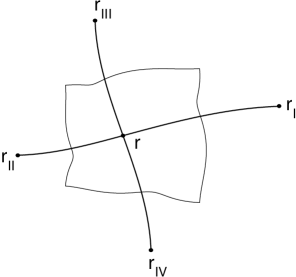
Figure 1: A lattice site, ${\bf r}$, on the distorted crystal and the four nearest neighbors are shown schematically. Also shown is the distorted unit cell of the central lattice site.

$${d[V({\bf r})P({\bf r},t})] = \frac{D_{0}\Delta t}{h^{2}}\bigg{[}V({\bf r}_{I})P({\bf r}_{I})+V({\bf r}_{II})P({\bf r}_{II})+$$ (1)

$$+V({\bf r}_{III})P({\bf r}_{III})+V({\bf r}_{IV})P({\bf r}_{IV})$$

$$-4V({\bf r})P({\bf r},t)\bigg{]}\ ,$$

where $h$ is the lattice spacing, $\Delta t$ is the small time increment, and $D_{0}$ is the diffusion coefficient. The volume of each, possibly distorted, unit cell is given by $V({\bf r})$. Equation (1) is exact and leads in the continuum limit to the general expression for diffusion in curved space Ikeda and Watanabe (1989). Although the crystal may be distorted, a regular crystal lattice can always be defined locally in terms of lattice coordinates $\sigma$. In the $\sigma$ space, the particle hops either up, down, left, or right. The correspondence is given by ${\bf r}_{I}\leftrightarrow{\mbox{\boldmath$\sigma$}}=(h,0)$, ${\bf r}_{II}\leftrightarrow{\mbox{\boldmath$\sigma$}}=(-h,0)$, ${\bf r}_{III}\leftrightarrow{\mbox{\boldmath$\sigma$}}=(0,h)$, and ${\bf r}_{IV}\leftrightarrow{\mbox{\boldmath$\sigma$}}=(0,-h)$. The positions of the neighboring sites are defined such that a hop in the appropriate direction leads to ${\bf r}$. For example,

$${\bf r}={\bf r}_{I}-h\left.\frac{\partial{\bf r}}{\partial\sigma_{1}}\right|_{{\bf r}_{I}}+\left.\frac{h^{2}}{2}\frac{\partial^{2}{\bf r}}{\partial\sigma_{1}^{2}}\right|_{{\bf r}_{I}}+O(h^{3})\ .$$ (2)

Note that the $\bf r$ coordinates are considered to be a fixed function of the $\sigma$ coordinates: ${\bf r}={\bf r}(\mbox{\boldmath$\sigma$})$. This mapping is independent of time, as the defects that generate the non-trivial mapping will be quenched in the two-dimensional crystal. Inverting eq. (2) for ${\bf r}_{I}$ gives

$${\bf r}_{I}={\bf r}+h\left.\frac{\partial{\bf r}}{\partial\sigma_{1}}\right|_{{\bf r}}+\left.\frac{h^{2}}{2}\frac{\partial^{2}{\bf r}}{\partial\sigma_{1}^{2}}\right|_{{\bf r}}+O(h^{3})\ .$$ (3)

With these expressions for the four neighboring sites, eq. (1) to $O(h)$ becomes

$$\frac{d[V({\bf r})P({\bf r},t)]}{dt} = \frac{D_{0}}{h^{2}}\bigg{[}h^{2}\frac{\partial^{2}r_{i}}{\partial\sigma_{\alpha}^{2}}\frac{\partial(VP)}{\partial r_{i}}$$ (4)

$$+h^{2}\frac{\partial r_{i}}{\partial\sigma_{\alpha}}\frac{\partial r_{j}}{\partial\sigma_{\alpha}}\frac{\partial^{2}(VP)}{\partial r_{i}\partial r_{j}}\bigg{]}\ ,$$

where the summation convention has been used. Equation (4) is exact and leads in the continuum limit to the general expression for diffusion in curved space Ikeda and Watanabe (1989). The notation

$$g^{ij}=\frac{\partial r_{i}}{\partial\sigma_{\alpha}}\frac{\partial r_{j}}{\partial\sigma_{\alpha}}$$ (5)

will be used. The shorthand $\partial_{i}=\partial/\partial r_{i}$ will also used. Equation (4) is a relation for the probability distribution in $\bf r$ space. The relation for the probability distribution in $\sigma$ space requires a Jacobian:

$$P({\bf r},t)=G(\mbox{\boldmath$\sigma$},t)|\det\partial\sigma_{\alpha}/\partial r_{i}|\ .$$ (6)

The Jacobian is given by

$$|\det\partial\sigma_{\alpha}/\partial r_{i}|=\sqrt{g}({\bf r})=\left|\frac{\partial\sigma_{x}}{\partial r_{x}}\frac{\partial\sigma_{y}}{\partial r_{y}}-\frac{\partial\sigma_{x}}{\partial r_{y}}\frac{\partial\sigma_{y}}{\partial r_{x}}\right|\ .$$ (7)

As noted, the Jacobian is $\sqrt{g}=(\det g_{ij})^{1/2}=1/(\det g^{ij})^{1/2}$, where the inverse of the matrix $g^{ij}$ is given by

$$g_{ij}=\frac{\partial\sigma_{\alpha}}{\partial r_{i}}\frac{\partial\sigma_{\alpha}}{\partial r_{j}}\ .$$ (8)

The volume of each unit cell is given by $V({\bf r})=h^{2}/\sqrt{g}({\bf r})$. By detailed balance, since the rates to hop forward and back between any two sites on the crystal are the same, the long-time average number of particles per site must be equal at all sites: $\lim_{t\to\infty}G(\mbox{\boldmath$\sigma$},t)={\rm const}$. This implies $\lim_{t\to\infty}P({\bf r},t)\propto\sqrt{g}({\bf r})$.

Since

$$\partial_{i}g^{ij} = \frac{\partial}{\partial r_{i}}\left(\frac{\partial r_{i}}{\partial\sigma_{\alpha}}\frac{\partial r_{j}}{\partial\sigma_{\alpha}}\right)$$ (9)

$$= \frac{\partial r_{j}}{\partial\sigma_{\alpha}}\frac{\partial}{\partial r_{i}}\frac{\partial r_{i}}{\partial\sigma_{\alpha}}+\frac{\partial r_{i}}{\partial\sigma_{\alpha}}\frac{\partial}{\partial r_{i}}\frac{\partial r_{j}}{\partial\sigma_{\alpha}}$$

$$= \frac{\partial r_{j}}{\partial\sigma_{\alpha}}\frac{\partial}{\partial r_{i}}\frac{\partial r_{i}}{\partial\sigma_{\alpha}}+\frac{\partial^{2}r_{j}}{\partial\sigma_{\alpha}^{2}}\ ,$$

eq. (4) becomes

$$\frac{\partial G}{\partial t}=D_{0}\left(\partial_{i}g^{ij}-\frac{\partial r_{j}}{\partial\sigma_{\alpha}}\frac{\partial}{\partial r_{i}}\frac{\partial r_{i}}{\partial\sigma_{\alpha}}\right)\partial_{j}G+D_{0}g^{ij}\partial_{i}\partial_{j}G\ .$$ (10)

Finally, given that

$$\frac{1}{\sqrt{g}}g^{ij}\partial_{i}\sqrt{g} = -\frac{1}{2}g^{ij}\partial_{i}\ln\det g^{-1}$$

$$= -\frac{1}{2}\frac{\partial r_{j}}{\partial\sigma_{\alpha}}\frac{\partial r_{i}}{\partial\sigma_{\alpha}}\frac{\partial\ln\det g^{-1}}{\partial r_{i}}$$

$$= -\frac{1}{2}\frac{\partial r_{j}}{\partial\sigma_{\alpha}}\frac{\partial\ln\det g^{-1}}{\partial\sigma_{\alpha}}\ ,$$

and

$$\frac{1}{2}\frac{\partial\ln\det g^{-1}}{\partial\sigma_{\alpha}} = \frac{1}{2}g_{ji}\frac{\partial g^{ij}}{\partial\sigma_{\alpha}}$$ (12)

$$= \frac{1}{2}\frac{\partial\sigma_{\beta}}{\partial r_{i}}\frac{\partial\sigma_{\beta}}{\partial r_{j}}\frac{\partial}{\partial\sigma_{\alpha}}\left(\frac{\partial r_{i}}{\partial\sigma_{\gamma}}\frac{\partial r_{j}}{\partial\sigma_{\gamma}}\right)$$

$$= \frac{\partial\sigma_{\beta}}{\partial r_{i}}\frac{\partial\sigma_{\beta}}{\partial r_{j}}\frac{\partial r_{j}}{\partial\sigma_{\gamma}}\frac{\partial}{\partial\sigma_{\alpha}}\frac{\partial r_{i}}{\partial\sigma_{\gamma}}$$

$$= \frac{\partial\sigma_{\beta}}{\partial r_{i}}\frac{\partial}{\partial\sigma_{\alpha}}\frac{\partial r_{i}}{\partial\sigma_{\beta}}$$

$$= \frac{\partial\sigma_{\beta}}{\partial r_{i}}\frac{\partial}{\partial\sigma_{\beta}}\frac{\partial r_{i}}{\partial\sigma_{\alpha}}~{}~{}~{}~{}~{}({\rm see~{}below})$$

$$= \frac{\partial}{\partial r_{i}}\frac{\partial r_{i}}{\partial\sigma_{\alpha}}\ ,$$

the final expression of the diffusion equation becomes

$$\frac{\partial G}{\partial t}=\frac{1}{\sqrt{g}}\partial_{i}(\sqrt{g}D_{0}g^{ij}\partial_{j}G)\ .$$ (13)

This equation applies everywhere except within the cores of topological defects, because it has been assumed in the second to last line of eq. (12) that the differentiations commute Seung and Nelson (1988). Equation (13) is nothing more than the usual diffusion equation in curved space, with the familiar Laplace-Beltrami operator Kreyszig (1991) replacing the Laplacian of flat space. The mean-square-displacement is given by

$$\left\langle r^{2}(t)\right\rangle = \int d{\bf r}|{\bf r}|^{2}P({\bf r},t)$$ (14)

$$= \int d{\bf r}\sqrt{g}({\bf r})|{\bf r}|^{2}G({\bf r},t)\ .$$ (15)

Equation (13) differs from the most general expression for diffusion in curved space by a term related to the torsion Ikeda and Watanabe (1989). We reevaluate the term $\partial\ln\det g/\partial r_{i}$:

$$\frac{1}{2}\frac{\partial\ln\det g}{\partial r_{i}} = \frac{1}{2}g^{kj}\frac{\partial}{\partial r_{i}}g_{jk}$$ (16)

$$= \frac{1}{2}\frac{\partial r_{k}}{\partial\sigma_{\alpha}}\frac{\partial r_{j}}{\partial\sigma_{\alpha}}\frac{\partial}{\partial r_{i}}\left(\frac{\partial\sigma_{\beta}}{\partial r_{j}}\frac{\partial\sigma_{\beta}}{\partial r_{k}}\right)$$

$$= \frac{\partial r_{k}}{\partial\sigma_{\alpha}}\frac{\partial r_{j}}{\partial\sigma_{\alpha}}\frac{\partial\sigma_{\beta}}{\partial r_{j}}\frac{\partial}{\partial r_{i}}\frac{\partial\sigma_{\beta}}{\partial r_{k}}$$

$$= \frac{\partial r_{k}}{\partial\sigma_{\alpha}}\frac{\partial}{\partial r_{i}}\frac{\partial}{\partial r_{k}}\sigma_{\alpha}$$

$$= \frac{\partial}{\partial\sigma_{\alpha}}\frac{\partial\sigma_{\alpha}}{\partial r_{i}}$$

$$+\frac{\partial r_{k}}{\partial\sigma_{\alpha}}\left(\frac{\partial}{\partial r_{i}}\frac{\partial}{\partial r_{k}}-\frac{\partial}{\partial r_{k}}\frac{\partial}{\partial r_{i}}\right)\sigma_{\alpha}$$

Defining the torsion as $2T_{ik}^{k}=(\partial r_{k}/\partial\sigma_{\alpha})(\partial^{2}/\partial r_{i}\partial r_{k}-\partial^{2}/\partial r_{k}\partial r_{i})\sigma_{\alpha}$, note that

$$g^{ij}\frac{1}{2}\frac{\partial\ln\det g}{\partial r_{i}} = \frac{\partial r_{i}}{\partial\sigma_{\alpha}}\frac{\partial r_{j}}{\partial\sigma_{\alpha}}\frac{\partial}{\partial\sigma_{\beta}}\frac{\partial\sigma_{\beta}}{\partial r_{i}}+2g^{ij}T_{ik}^{k}$$ (17)

$$= \frac{\partial r_{j}}{\partial\sigma_{\alpha}}\frac{\partial r_{i}}{\partial\sigma_{\alpha}}\frac{\partial}{\partial\sigma_{\beta}}\frac{\partial\sigma_{\beta}}{\partial r_{i}}+2g^{ij}T_{ik}^{k}$$

$$= -\frac{\partial r_{j}}{\partial\sigma_{\alpha}}\frac{\partial\sigma_{\beta}}{\partial r_{i}}\frac{\partial}{\partial\sigma_{\beta}}\frac{\partial r_{i}}{\partial\sigma_{\alpha}}+2g^{ij}T_{ik}^{k}$$

$$= -\frac{\partial r_{j}}{\partial\sigma_{\alpha}}\frac{\partial}{\partial r_{i}}\frac{\partial r_{i}}{\partial\sigma_{\alpha}}+2g^{ij}T_{ik}^{k}$$

Combining eqs. (10), (LABEL:5aa), and (17), we find that the exact expression for the diffusion equation is

$$\frac{\partial G}{\partial t}=\frac{1}{\sqrt{g}}\partial_{i}(\sqrt{g}D_{0}g^{ij}\partial_{j}G)-2D_{0}g^{ij}T_{ik}^{k}\partial_{j}G\ .$$ (18)

Equation (18) is equal to the general expression for diffusion in curved space Ikeda and Watanabe (1989). The difference between the exact answer, eq. (18), and that assuming that the order of differentiation commutes, eq. (13), is given by the torsion term. The torsion is an explicit measure of the non-commutativity of differentiation and is, therefore, a measure of the defect density Seung and Nelson (1988). The diffusion equation does not apply within the cores of defects, where the metric tensor is undefined, and the only place where the torsion is non-zero. The effects of the torsion should probably be studied with a detailed model rather than with the long-wavelength, continuum theory of the diffusion equation. For this reason, we exclude this torsion term (although see section VII below). The long range, external to defect core, effects of the topological defects are, of course, included in eq. (13) through the metric tensor $g^{ij}$ and $\sqrt{g}$. Refs. Bausch et al. (1994); Krukowski and Turski (1993) included the torsion term explicitly, and a series of approximations allowed the generation of non-physical dynamics.

Equation (13) can, alternatively, be derived by consideration of the field-theoretic representation of the diffusion operator Lee (1994); Lee and Cardy (1995). In this representation, the Green function is given by an average over a field:

$$G({\bf r},t)=\left\langle a({\bf r},t)\right\rangle\ ,$$ (19)

where the average is taken with respect to the weight $\exp(-S)$. The particle hopping occurs in $\sigma$ space without regard to the distortion of the crystal, as the rate of hopping is independent of the distance between lattice sites. The action for such normal diffusion is given by

$$``S = \int_{0}^{\infty}dt\int d\mbox{\boldmath$\sigma$}\left\{\bar{a}[\partial_{t}+\delta(t)]a-D_{0}\bar{a}\frac{\partial^{2}a}{\partial\sigma_{\alpha}^{2}}\right\}$$ (20)

$$+\int d\mbox{\boldmath$\sigma$}n_{0}(\mbox{\boldmath$\sigma$})\bar{a}({\bf r},0)\ ,^{\prime\prime}$$

where $n_{0}$ is the initial density profile, and details of the replica indices used to accommodate averaging over disorder have been suppressed Kravtsov et al. (1985); Park and Deem (1998b). This action is enclosed in quotations since the $\sigma$ space is not well-defined in the presence of topological defects. That the diffusion is normal in $\sigma$ space, however, does make it clear that the limiting distribution should be $\lim_{t\to\infty}G(\mbox{\boldmath$\sigma$},t)=({\rm const})$. From eq. (6), then, the limiting distribution in ${\bf r}$ space is given by $\lim_{t\to\infty}P({\bf r},t)=({\rm const})\sqrt{g}({\bf r})=\sqrt{g}({\bf r})/\int d{\bf r}^{\prime}\sqrt{g}({\bf r}^{\prime})$. While this result may be surprising, note that the defects which distort the geometry must affect the limiting distribution, unlike the typical case in differential geometry where the observables are described by a theory independent of the coordinate system. This explicit result for the limiting distribution agrees with the prediction from the simple detailed balance argument given above. Note that $\int d{\bf r}\sqrt{g}({\bf r})$ is a constant for a given realization of the quenched disorder. The long-time normalization factor for the probability is fixed to be the inverse of this integral by the initial condition $P({\bf r},0)=\delta({\bf r})$. Equation (13) for the dynamics conserves $\int d{\bf r}\sqrt{g}({\bf r})G({\bf r},t)$, hence, the probability distribution, $P({\bf r},t)=\sqrt{g}({\bf r})G({\bf r},t)$, remains normalized to unity for all times $t\geq 0$. After change of variables from $\sigma$ to ${\bf r}$, again making the assumption of being outside defect cores so that differentiation commutes, the action becomes

$$S = \int_{0}^{\infty}dt\int d{\bf r}\left\{\sqrt{g}\bar{a}[\partial_{t}+\delta(t)]a-\bar{a}\partial_{i}[\sqrt{g}D_{0}g^{ij}\partial_{j}a]\right\}$$ (21)

$$+\int d{\bf r}\sqrt{g}n_{0}({\bf r})\bar{a}({\bf r},0)\ .$$

Finally, integrating out the $\bar{a}$ field, using eq. (19), and noting that for the Green function $n_{0}(\mbox{\boldmath$\sigma$})=\delta(\mbox{\boldmath$\sigma$})$, the Fokker-Planck equation is

$$\frac{\partial G}{\partial t}=\frac{1}{\sqrt{g}}\partial_{i}(\sqrt{g}D_{0}g^{ij}\partial_{j}G)\ ,$$ (22)

with $G({\bf r},0)=\delta({\bf r})/\sqrt{g}({\bf r})$. The field-theoretic result, eq. (22), is the same as that derived by more physically-motivated means, eq. (13).

III The Model of Topological Disorder

The topological defects modify the diffusive motion of the particle by affecting the $g^{ij}$ in the Fokker-Planck equation. Once $g^{ij}$ is determined, eqs. (13) and (15) provide the means to calculate the transport properties. It is conventional in continuum elasticity theory to relate the spatial coordinates to the lattice coordinates by

$${\bf r}(\mbox{\boldmath$\sigma$})=\mbox{\boldmath$\sigma$}+{\bf u}({\bf r})\ ,$$ (23)

where the displacement field ${\bf u}$ is written in terms of the ${\bf r}$ variables that remain well-defined even in the presence of topological defects. The $\sigma$ space, on the other hand, does not remain well-defined, since the effect of disclinations is to add or remove wedges of lattice sites from $\sigma$ space, and the effect of dislocations is to add or remove half-lines of lattice sites from $\sigma$ space. For a dislocation at the origin with Burgers vector b, the displacement fields are given by Nabarro (1987)

$$2\pi u_{i}^{\rm disloc} = -\frac{(\mu+\lambda)}{(2\mu+\lambda)}\frac{\epsilon_{kl}b_{l}r_{i}r_{k}}{r^{2}}+b_{i}\tan^{-1}\frac{r_{y}}{r_{x}}$$ (24)

$$-\frac{\mu}{2\mu+\lambda}\epsilon_{li}b_{l}\ln{\frac{r}{h}}\ ,$$

where $\mu$ and $\lambda$ are the two-dimensional Lamé coefficients, $\epsilon_{11}=\epsilon_{22}=0$, and $\epsilon_{12}=-\epsilon_{21}=1$. Similarly, for a disclination of strength $s$ at the origin, the displacement fields are given by

$$2\pi u^{\rm disclin}_{i} = -\frac{(\mu+\lambda)}{2(2\mu+\lambda)}sr_{i}-s\epsilon_{ik}r_{k}\tan^{-1}{\frac{r_{y}}{r_{x}}}$$ (25)

$$+\frac{\mu}{2\mu+\lambda}sr_{i}\ln(r/h)\ .$$

Equation (25) differs from the simplified distortion field used in Bausch et al. (1994) by the inclusion of the strain field representing the local lattice contraction and expansion. These are the terms in eq. (25) that depend on the Lamé coefficients. Since linear elasticity theory is used, the dislocation field is given by the dipole limit of two superimposed disclination fields:

$$u^{\rm disloc}_{i}=(b_{l}/s)\epsilon_{jl}\partial_{j}u^{\rm disclin}_{i}+{\rm const}\ .$$ (26)

The derivatives of the displacement fields are required to evaluate $g^{ij}$ from eq. (5). The dislocation fields are preferable for this calculation, as they lead to well-defined Fourier transforms:

$$\hat{\partial_{x}u_{x}}{}^{\rm disloc} = i\left[\frac{\mu+\lambda}{2\mu+\lambda}\frac{2k_{x}^{2}k_{y}}{k^{4}}-\frac{k_{y}}{k^{2}}\right]\hat{b}_{x}({\bf k})$$

$$+i\left[\frac{\mu+\lambda}{2\mu+\lambda}\frac{k_{x}(-k_{x}^{2}+k_{y}^{2})}{k^{4}}+\frac{\mu}{2\mu+\lambda}\frac{k_{x}}{k^{2}}\right]\hat{b}_{y}({\bf k})$$

$$\hat{\partial_{y}u_{x}}{}^{\rm disloc} = i\left[\frac{\mu+\lambda}{2\mu+\lambda}\frac{2k_{x}k_{y}^{2}}{k^{4}}+\frac{k_{x}}{k^{2}}\right]\hat{b}_{x}({\bf k})$$

$$+i\left[\frac{\mu+\lambda}{2\mu+\lambda}\frac{k_{y}(-k_{x}^{2}+k_{y}^{2})}{k^{4}}+\frac{\mu}{2\mu+\lambda}\frac{k_{y}}{k^{2}}\right]\hat{b}_{y}({\bf k})$$

$$\hat{\partial_{x}u_{y}}{}^{\rm disloc} = i\left[\frac{\mu+\lambda}{2\mu+\lambda}\frac{k_{x}(-k_{x}^{2}+k_{y}^{2})}{k^{4}}-\frac{\mu}{2\mu+\lambda}\frac{k_{x}}{k^{2}}\right]\hat{b}_{x}({\bf k})$$

$$+i\left[-\frac{\mu+\lambda}{2\mu+\lambda}\frac{2k_{x}^{2}k_{y}}{k^{4}}-\frac{k_{y}}{k^{2}}\right]\hat{b}_{y}({\bf k})$$

$$\hat{\partial_{y}u_{y}}{}^{\rm disloc} = i\left[\frac{\mu+\lambda}{2\mu+\lambda}\frac{k_{y}(-k_{x}^{2}+k_{y}^{2})}{k^{4}}-\frac{\mu}{2\mu+\lambda}\frac{k_{y}}{k^{2}}\right]\hat{b}_{x}({\bf k})$$ (27)

$$+i\left[-\frac{\mu+\lambda}{2\mu+\lambda}\frac{2k_{x}k_{y}^{2}}{k^{4}}+\frac{k_{x}}{k^{2}}\right]\hat{b}_{y}({\bf k})\ .$$

Note that the $x$ and $y$ derivatives of the strain fields are not simply related by the ratio $k_{x}/k_{y}$, due to the presence of the defects. The linearity of elasticity theory has been used to accommodate a density field of defects with Burgers vectors given by ${\bf b}({\bf r})$.

The dislocations are assumed to be distributed randomly in the material with correlation function

$$\left\langle\hat{b}_{i}({\bf k}_{1})\hat{b}_{j}({\bf k}_{2})\right\rangle=\delta_{ij}(2\pi)^{2}\delta({\bf k}_{1}+{\bf k}_{2})\hat{\chi}({\bf k}_{1}+{\bf k}_{2})\ ,$$ (28)

where

$$\hat{\chi}({\bf k})=\gamma k^{n}\exp(-\beta k^{2})\ .$$ (29)

Physically, we expect this model of dislocations should generate identical dynamics to one in which disclinations are randomly distributed with correlation function

$$\left\langle\hat{s}({\bf k}_{1})\hat{s}({\bf k}_{2})\right\rangle=(2\pi)^{2}\delta({\bf k}_{1}+{\bf k}_{2})|{\bf k}_{1}+{\bf k}_{2}|^{2}\hat{\chi}({\bf k}_{1}+{\bf k}_{2})\ .$$ (30)

This physical expectation is a mathematical consequence of eq. (26).

With these results in hand, we are now in a position to calculate the action for the field theoretic description of the Green function. The terms in eq. (21) are expressed to linear and quadratic order in $u^{\rm disloc}$, and then an average over the random distribution of dislocations is taken. In fact, since eq. (14) is preferable to eq. (15), the theory is written in terms of the fields $\bar{a},c$, where $c=\sqrt{g}a$, and $P=\langle c\rangle$. The action is

$$S = \int_{0}^{\infty}dt\int d{\bf r}\bar{a}[\partial_{t}-(D_{0}+\delta D_{II})\nabla^{2}+\delta(t)]c$$ (31)

$$+\int d{\bf r}\delta({\bf r})\bar{a}({\bf r},0)+S_{I}\ ,$$

where

$$S_{I} = -2D^{2}\int dt_{1}dt_{2}\int_{{\bf k}_{1}{\bf k}_{2}{\bf k}_{3}{\bf k}_{4}}$$ (32)

$$\times(2\pi)^{2}\delta({\bf k}_{1}+{\bf k}_{2}+{\bf k}_{3}+{\bf k}_{4})$$

$$\times\hat{\bar{a}}({\bf k}_{1},t_{1})\hat{c}({\bf k}_{2},t_{1})\hat{\bar{a}}({\bf k}_{3},t_{2})\hat{c}({\bf k}_{4},t_{2})$$

$$\times\bigg{[}\frac{\mu}{2\mu+\lambda}k_{1}^{2}+\frac{\mu+\lambda}{2\mu+\lambda}\frac{{\bf k}_{1}\cdot{\bf k}_{2}(k_{1}^{2}+k_{2}^{2})+2k_{1}^{2}k_{2}^{2}}{|{\bf k}_{1}+{\bf k}_{2}|^{2}}\bigg{]}$$

$$\times\bigg{[}\frac{\mu}{2\mu+\lambda}k_{3}^{2}+\frac{\mu+\lambda}{2\mu+\lambda}\frac{{\bf k}_{3}\cdot{\bf k}_{4}(k_{3}^{2}+k_{4}^{2})+2k_{3}^{2}k_{4}^{2}}{|{\bf k}_{3}+{\bf k}_{4}|^{2}}\bigg{]}$$

$$\times\frac{\hat{\chi}({\bf k}_{1}+{\bf k}_{2})}{|{\bf k}_{1}+{\bf k}_{2}|^{2}}\ ,$$

where the notation $\int_{\bf k}$ stands for $\int d^{2}{\bf k}/(2\pi)^{2}$. The term resulting from a non-zero average of $(u^{\rm disloc})^{2}$ is

$$\delta D_{II} = \frac{\gamma D_{0}}{2\pi}\left[\frac{13\lambda^{2}+16\mu\lambda+25\mu^{2}}{9(2\mu+\lambda)^{2}}\right]$$

$$\times\int_{0}^{\infty}dk~{}k^{n-1}\exp(-\beta k^{2})$$

$$= \frac{\gamma D_{0}}{2\pi}\frac{\Gamma(n/2)}{2\beta^{n/2}}\left[\frac{13\lambda^{2}+16\mu\lambda+25\mu^{2}}{9(2\mu+\lambda)^{2}}\right]\ .$$

Exactly the same theory is generated if the correlation function eq. (30) is used with the disclination displacements given by eq. (25).

IV Topological Disorder Reduces the Diffusion Constant

For the model with $n>0$, the topological disorder reduces the diffusion coefficient by a finite amount. The finite contribution of $\delta D_{II}$ is explicit in eq. (LABEL:21). Moreover, standard power counting arguments Zinn-Justin (1996) show that non-perturbative, renormalization effects can be expected from eq. (32) only for $n\leq 0$. From perturbation theory on eq. (32) for $n>0$, the contribution to the diffusion coefficient is found to be

$$\delta D_{I}=-\frac{\gamma D_{0}}{2\pi}\frac{\Gamma(n/2)}{2\beta^{n/2}}\left[\frac{4\mu^{2}+2(\mu+\lambda)^{2}}{(2\mu+\lambda)^{2}}\right]\ .$$ (34)

The total contribution to the diffusion coefficient is, therefore,

$$\delta D=-\frac{\gamma D_{0}}{2\pi}\frac{\Gamma(n/2)}{2\beta^{n/2}}\left[\frac{29\mu^{2}+20\mu\lambda+5\lambda^{2}}{9(2\mu+\lambda)^{2}}\right]\ .$$ (35)

To demonstrate the behavior of this model, we perform numerical simulations. The dislocation density fields are constructed with correlation function eq. (28) for $n=2$ using the method of ref. Pham and Deem (1998). Equation (27) and an inverse fast Fourier transform are used to calculate the displacement fields in real space. The matrix $g^{ij}$ is calculated as the inverse of the matrix $g_{ij}$ given by eq. (8), and the relation $\mbox{\boldmath$\sigma$}={\bf r}-{\bf u}({\bf r})$ is used.

The Fokker-Planck equation, eq. (13), can be considered to result from many small hops, the net effect of which is Gaussian, diffusive motion. So that a hopping process on a lattice reproduces this differential equation, the average and mean-square displacements must be correct at each lattice site. Interestingly, this differential equation can be evaluated by Monte Carlo methods on a perfect, square lattice, even though the differential equation itself describes the motion of a particle in a distorted geometry. To first order in the time step, the mean displacement is given by

$$\left\langle r_{i}(\Delta t)\right\rangle = \int d{\bf r}\sqrt{g}~{}r_{i}G({\bf r},\Delta t)$$ (36)

$$= \int_{0}^{\Delta t}dt\int d{\bf r}\sqrt{g}~{}r_{i}\partial_{t}G({\bf r},t)$$

$$+\int d{\bf r}\sqrt{g}~{}r_{i}G({\bf r},0)$$

$$= \frac{D_{0}\Delta t}{\sqrt{g}}\partial_{j}(\sqrt{g}g^{ij})\ ,$$

where eq. (13) and integration by parts twice has been used in the last step. Similarly, to first order, the mean-square displacement is given by

$$\left\langle r_{i}(\Delta t)r_{j}(\Delta t)\right\rangle = \int d{\bf r}\sqrt{g}~{}r_{i}r_{j}G({\bf r},\Delta t)$$ (37)

$$= \int_{0}^{\Delta t}dt\int d{\bf r}\sqrt{g}~{}r_{i}r_{j}\partial_{t}G({\bf r},t)$$

$$+\int d{\bf r}\sqrt{g}~{}r_{i}r_{j}G({\bf r},0)$$

$$= 2D_{0}\Delta tg^{ij}\ ,$$

where eq. (13) and integration by parts twice has again been used in the last step.

Eight hopping rates are defined, consistent with the specifications of eqs. (36–37). So that the non-diagonal terms of $g^{ij}$ are properly reproduced, both nearest- and next-nearest-neighbor hops are required. The rate for each hopping event is

$$T_{i}({\bf r}\to{\bf r}+\Delta{\bf r})=\frac{D_{0}}{h^{2}}\left[\frac{g({\bf r}+\Delta{\bf r})}{g({\bf r})}\right]^{1/4}$$

$$\times\frac{1}{2}\left[f({\bf r})+f({\bf r}+\Delta{\bf r})\right]\ .$$ (38)

The function $f$ is given by

$$f = g^{11}-\epsilon,{\rm~{}for~{}}\Delta{\bf r}=(\pm h,0)$$

$$f = g^{22}-\epsilon,{\rm~{}for~{}}\Delta{\bf r}=(0,\pm h)$$

$$f = (g^{12}+\epsilon)/2,{\rm~{}for~{}}\Delta{\bf r}=(\pm h,\pm h)$$

$$f = (-g^{12}+\epsilon)/2,{\rm~{}for~{}}\Delta{\bf r}=(\pm h,\mp h)\ ,$$ (39)

with $\epsilon=|g^{12}|$. The transition rates in eq. (38) explicitly satisfy detailed balance for the equilibrium distribution $\lim_{t\to\infty}P({\bf r},t)=(\rm const)\sqrt{g}({\bf r})$. These rates give the correct average and mean-square displacements to $O(h)$, eqs. (36–37), when $\Delta t=1/(\sum_{i}T_{i})$. These results imply that the Monte Carlo procedure evaluates the differential eq. (4), and so eq. (14) can be used to calculate the mean-square-displacements. The procedure of ref. Pham and Deem (1998) is used to perform the simulation of this random process, where the particle is moved to one of the neighboring eight sites with probability $\Delta tT_{i}$, and time is incremented by $dt=-\Delta t\ln(x)$, where $x$ is a uniform random number, $0<x\leq 1$.

The results of the numerical simulations are shown in Fig. 2. The calculations were performed for the case $\mu=\lambda$, $n=2$, $h=1$, and $\beta=4$. The simulations were done on $4096\times 4096$ lattices for a total of 500000 steps and averaged over 100000 particles. The strength of the disorder was varied between $0<\gamma<1.25$. For larger values of $\gamma$, the transition rates specified by eqs. (38–39) became negative at some of the lattice sites. Also shown is a fit to the functional form $\delta D/D_{0}=1-ax$. The fit to the simulation data of $a=0.01285\pm 0.0051$ is in excellent agreement with the theoretical of result $a=0.01326$ from eq.  (35).

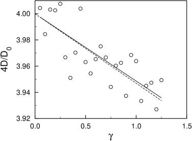
Figure 2: Shown are simulation results for the reduction in the diffusion coefficient for the case $n=2$, $\mu=\lambda$, and $\beta=4$. The error bars are roughly $\pm 0.01$. The best linear fit to the simulation data is shown (solid line). The simulation data are compared to perturbation theory (dashed line), eq. 35, $\delta D/D_{0}=-\gamma/(6\pi\beta)$.

V Possible Anomalous Diffusion

The case $n=0$ is interesting, as perturbation theory for the diffusion coefficient formally diverges. While this theory has the same upper critical dimension, $d_{c}=2$, as the problem of diffusion of an ion in the electrostatic field of random, quenched charges Bouchaud and Georges (1990), the interaction term, eq. (32), is quite different. In comparison to the analogous term for diffusion in the random potential (e.g. term $S_{3}$ of ref. Park and Deem (1998b) with $\hat{\chi}_{vv}(k)=\hat{\chi}(k)/k^{2}$), the term proportional to $\mu$ is new, as are the factors $-k_{1}^{2}+2[k_{1}^{2}k_{2}^{2}-({\bf k}_{1}\cdot{\bf k}_{2})^{2}]/|{\bf k}_{1}+{\bf k}_{2}|^{2}$ in the term proportional to $\mu+\lambda$. Indeed, as we will see, the present interaction term is more difficult to analyze than is the analogous one from diffusion in a random potential. Formally, the case of $n\leq 0$ leads to large distortions of the lattice for arbitrarily small $\gamma$, which implies that the assumption of linear elasticity used to calculate the strain fields breaks down. We can, however, treat the dynamical behavior implied by eqs. (31–32) as an interesting mathematical question. A technical detail is that we supplement the correlation function eq. (29) with the condition $\hat{\chi}({\bf 0})\equiv 0$ so that the displacement fields of eq. (27) are well-defined for $k=0$. This suppresses macroscopic size fluctuations of the sample.

Before applying renormalization group theory, the terms in the field theory must be known. The quartic interaction term, eq. (32), is known. The contribution to the propagator, eq. (LABEL:21), while explicit, leads to a formal divergence of the short-time diffusion coefficient. Numerical simulations show that the local diffusivity tensor, $D_{0}g^{ij}$, can be large but is never vanishingly small. The locations of large local diffusivity, moreover, are isolated. The apparent divergence of $\delta D_{II}$ is, thus, simply the result of particles rapidly hopping away from a few isolated locations. These physical considerations suggest that the divergence of $\delta D_{II}$ is washed out by spatial averaging and is not important for the long-time dynamics. We can, therefore, assume a finite local diffusivity. Numerical simulations of the dynamics, to be described below, bear out this assumption of a finite short-time diffusivity. Indeed, a finite short-time diffusivity is assured for finite lattice sizes by the elimination of the $\hat{\chi}({\bf 0})$ mode. The anomalous dynamics, then, is observed on finite lattices for time scales that are less than the characteristic time it takes to travel across the lattice.

We apply renormalization group theory to the action (31–32) to take into account the effects of nonzero $\gamma$. To one-loop order, self-energy and vertex diagrams are summarized in Figs. 3 and 4.

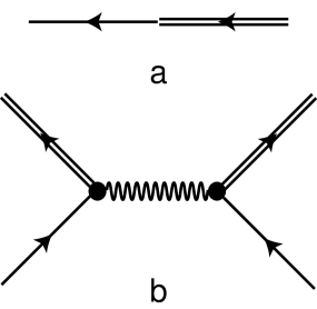
Figure 3: a) Diagram representing the propagator. The arrow points in the direction of increasing time, and double lines represent the bar fields. b) Disorder vertex $\gamma$.

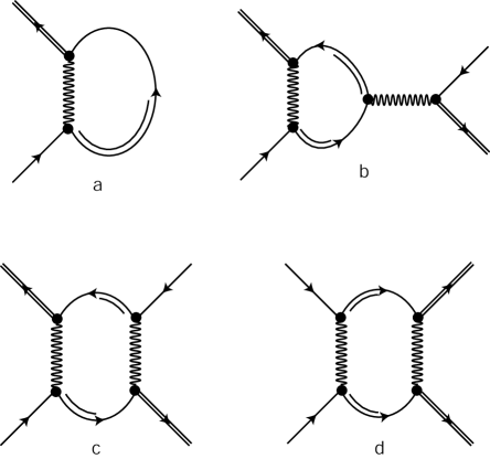
Figure 4: One-loop diagrams: a) self-energy diagrams contributing to $D$. b,c,d) vertex diagrams contributing to $\gamma$. Diagrams (c) and (d) cancel.

The flow equations are integrated to a time small enough so that perturbation theory applies. In this regime, matching theory is used to determine the constants of integration for the flow equations. Momenta in the range $\Lambda/b<k<\Lambda$ are integrated over, and the fields are rescaled by $\hat{\bar{a}}^{\prime}(b{\bf k},b^{-z}t)=\hat{\bar{a}}({\bf k},t)/\bar{\alpha}$ and $\hat{c}^{\prime}(b{\bf k},b^{-z}t)=\hat{c}({\bf k},t)/\alpha$. The relations $\alpha=1,\bar{\alpha}=b^{2}$ are used to achieve a fixed point and to keep the time derivative in $S$ constant. The flow parameter is defined by $l=\ln b$. We determine the dynamical exponent, $z$, by requiring that the diffusion coefficient remain unchanged. Defining $\gamma_{1}^{2}=\gamma\mu^{2}/(2\mu+\lambda)^{2}$, $\gamma_{2}^{2}=\gamma\mu(\mu+\lambda)/[2(2\mu+\lambda)^{2}]$, and $\gamma_{3}^{2}=\gamma(\mu+\lambda)^{2}/[4(2\mu+\lambda)^{2}]$, the contributions to the parameters from the one-loop diagrams of fig. 4 are

$$\frac{d\ln D}{dl} = z-2-\frac{2}{\pi}(\gamma_{1}^{2}+2\gamma_{3}^{2})$$

$$\frac{d\ln\gamma_{1}^{2}}{dl} = 2(z-2)-\frac{4}{\pi}(\gamma_{1}^{2}+2\gamma_{3}^{2})$$

$$\frac{d\ln\gamma_{2}^{2}}{dl} = 2(z-2)-\frac{2}{\pi}(\gamma_{1}^{2}+3\gamma_{3}^{2}-2\gamma_{1}\gamma_{3})$$

$$\frac{d\ln\gamma_{3}^{2}}{dl} = 2(z-2)-\frac{4}{\pi}(\gamma_{3}^{2}-2\gamma_{1}\gamma_{3})\ .$$ (40)

From the requirement that the diffusion coefficient remain fixed, the dynamical exponent is

$$z=2+\frac{2}{\pi}(\gamma_{1}^{2}+2\gamma_{3}^{2})\ .$$ (41)

Using eq. (41) in eq. (40), the flow equations become

$$\frac{d\ln\gamma_{1}^{2}}{dl} = 0$$

$$\frac{d\ln\gamma_{2}^{2}}{dl} = \frac{2}{\pi}(\gamma_{1}+\gamma_{3})^{2}$$

$$\frac{d\ln\gamma_{3}^{2}}{dl} = \frac{4}{\pi}(\gamma_{1}+\gamma_{3})^{2}\ .$$ (42)

As expected, the flow equations show that there are only two independent parameters, $\gamma_{1}$ and $\gamma_{3}$, resulting from renormalization of the two Lamé coefficients. In other words, the relation $\gamma_{2}^{2}(l)=\gamma_{1}(l)\gamma_{3}(l)$ is maintained under the renormalization.

Unexpectedly, however, the flow equations show that the $\gamma_{2}(l)$ and $\gamma_{3}(l)$ are growing. Indeed, these one-loop flow equations predict $\gamma_{3}(l)$ flows to infinity at a finite time corresponding to $l=[\pi/(2\gamma_{1}^{0})^{2}]\{\ln[(\gamma_{1}^{0}+\gamma_{3}^{0})/\gamma_{3}^{0}]-\gamma_{1}^{0}/(\gamma_{1}^{0}+\gamma_{3}^{0})\}$. The divergence of this parameter implies that higher order terms must be kept in the flow equation to derive a controlled result. It may also be the case that terms higher order in $u^{\rm disloc}$ must be kept in the expansion of the action (21).

If the renormalization of the parameters is assumed to be controlled by higher-loop corrections and small, the dynamical exponent can be used to determine the scaling exponent for the mean-square displacement at long times:

$$\left\langle r^{2}(t)\right\rangle\sim({\rm const})t^{1-\delta}\ .$$ (43)

The renormalized time flows as

$$t(l^{*})=te^{-\int_{0}^{l^{*}}z(l)dl}=t_{0}\ ,$$ (44)

where the flow equations are stopped at $l^{*}$ so that $t_{0}\approx h^{2}/(4D_{0})$. The renormalized mean-square displacement flows as

$$\left\langle r^{2}(t)\right\rangle=e^{2l}\left\langle r^{2}[t(l),l]\right\rangle\ .$$ (45)

Finally, at the matching

$$\left\langle r^{2}[t(l^{*}),l^{*}]\right\rangle=4Dt(l^{*})\ ,$$ (46)

since the time is short enough so that the disorder does not significantly affect the motion of the particle. In other words, it is assumed that at short times the diffusion coefficient remains finite, despite the formal appearance of $\delta D_{II}$ in eq. (LABEL:21). Putting these matching results together with the dynamical exponent, the mean-square displacement is found to scale at long times as

$$\left\langle r^{2}(t)\right\rangle\sim({\rm const})t^{1/[1+(\gamma_{1}^{2}+2\gamma_{3}^{2})/\pi]}\ .$$ (47)

To test whether anomalous scaling occurs in the full non-linear model, we perform numerical simulations. The transition rates from eqs. (38–39) cannot be used, as they are negative even for small values of $\gamma$. We, therefore, develop a new strategy based upon the idea that diffusion locally follows a Gaussian probability distribution with mean and variance specified by eqs. (36–37). The time increment $\Delta t$ is chosen so that $\max(|\langle\delta r_{i}\rangle|,|\langle\delta r_{i}\delta r_{j}\rangle|)$ is on the order of unity. This is done by choosing $1/\Delta t$ to be the maximum of the absolute values of the two average displacements in eq. (36) and the two eigenvalues of the matrix $D_{0}g^{ij}$. Defining the matrix $w=(2D_{0}\Delta tg^{ij})^{1/2}$, the random displacements of the diffusing particle are given by the relations

$$\Delta x = \frac{D_{0}\Delta t}{\sqrt{g}}\partial_{j}(\sqrt{g}g^{1j})+w^{11}z_{1}+w^{12}z_{2}$$

$$\Delta y = \frac{D_{0}\Delta t}{\sqrt{g}}\partial_{j}(\sqrt{g}g^{2j})+w^{21}z_{1}+w^{22}z_{2}\ ,$$ (48)

where $z_{1}$ and $z_{2}$ are independent, Gaussian random variables with zero mean and unit variance. This approach reproduces the Fokker-Planck equation (4) in the limit of a small lattice spacing and time increment. For a finite lattice spacing, the diffusion coefficient, and possibly the scaling exponent $\delta$, contain discretization errors.

The results of numerical simulations with this scheme are shown in Fig. 5. The calculations were performed for the case $\mu=\lambda$, $n=0$, $h=1$, and $\beta=4$. The simulations were done on $4096\times 4096$ lattices for a total of 1000000 steps and averaged over 100000 particles. Also shown is a fit to the functional form of eq. (43). The simulation results are approximately fit by $(z-2)/\gamma=1.02\pm 0.28$. If it is assumed that none of the parameters flow, the scaling exponent is given by $(z-2)/\gamma=2/(3\pi)\approx 0.2122$. By comparison, the simulation results suggest that there is substantial positive renormalization of the parameters, as is suggested by eq. (42).

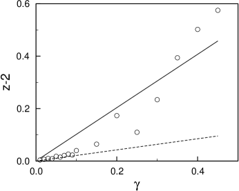
Figure 5: Shown are simulation results for the scaling exponent for the case $n=0$, $\mu=\lambda$, and $\beta=4$. The error bars are given roughly by the scatter in the data. The best linear fit to the simulation data is shown (solid line). Also shown (dashed line) is the prediction assuming that the other parameters do not flow, $z=2+2\gamma/(3\pi)$.

VI Discussion

A Fokker-Planck equation for diffusion on the surface of a crystal with topological defects, eq. (13), has been derived by two independent methods. As expected, the usual diffusion equation in curved space is derived. An additional assumption of $\sqrt{g}=1$ of previous, approximate treatments Bausch et al. (1994) has also been removed in the present calculation through the use of the exact strain field eq. (25). The theory of random dislocations is shown to be equivalent to a theory of random disclinations, where a simple factor of $k^{2}$ relates the correlation functions of the two models of disorder, eqs. (28) and (30).

The field theory for disorder, eqs. (31–32), is explicitly shown to be distinct from that for diffusion of an ion in a random electrostatic potential field. One consequence of this difference is that the renormalization group flow equations are more involved to analyze, with one-loop results unable to render a controlled prediction.

Topological disorder slows down a diffusing particle, as shown by eq. (35). This reduced transport should be observable on the surfaces of crystals with quenched disclination or dislocation defects. While the effect is subtle, it would be an interesting one to observe experimentally. The present computer simulation results suggest such observations should be feasible.

For singular disorder, $n\leq 0$ in two dimensions, the model of topological disorder leads to subdiffusive motion of the particle. Of course, for such singular disorder, the assumption of linear elasticity breaks down. Moreover, the energy of a distribution of topological defects with net dipole moment becomes super-extensive due to large strain fields at the edges of the two-dimensional crystal Seung and Nelson (1988). Nonetheless, the suggestion that subdiffusion is the mathematical result of motion in the, possibly approximate, random displacement fields of linear elasticity theory is interesting. Renormalization group arguments are suggestive of such subdiffusion, although one-loop results are unable to capture the exponents quantitatively.

Numerical simulations accurate to all orders in the displacement fields suggest that the motion is, indeed, subdiffusive. These numerical simulations suggest that there is significant renormalization of the disorder strength parameter, in contrast to the case of diffusion in random potential fields Bouchaud and Georges (1990). Interestingly, the renormalization of $z$ appears less significant for smaller values of $\gamma$, although this may be because the crossover time for renormalization is large for small $\gamma$ and longer than the observed simulation time. These simulations suggest a power law behavior of the mean square displacement, although localization at exceptionally long times cannot be ruled out, in principle.

VII What if Torsion is Included?

We here comment on the impact of the torsion term within the continuum theory of the diffusion equation. The torsion term is evaluated as

$$2T_{ik}^{k}\equiv T_{i} = \left(\frac{\partial r_{k}}{\partial\sigma_{\alpha}}\right)\left(\frac{\partial^{2}}{\partial r_{i}\partial r_{k}}-\frac{\partial^{2}}{\partial r_{k}\partial r_{i}}\right)\sigma_{\alpha}$$ (49)

$$= -\epsilon_{ij}\frac{\partial r_{j}}{\partial\sigma_{\alpha}}b_{\alpha}\ .$$

Expanding eq. (18) to linear order in $u^{\rm disloc}$, we find that the interaction term, previously eq. (32), becomes

$$S_{I} = \frac{D^{2}}{2}\int dt_{1}dt_{2}\int_{{\bf k}_{1}{\bf k}_{2}{\bf k}_{3}{\bf k}_{4}}$$ (50)

$$\times(2\pi)^{2}\delta({\bf k}_{1}+{\bf k}_{2}+{\bf k}_{3}+{\bf k}_{4})$$

$$\times\hat{\bar{a}}({\bf k}_{1},t_{1})\hat{c}({\bf k}_{2},t_{1})\hat{\bar{a}}({\bf k}_{3},t_{2})\hat{c}({\bf k}_{4},t_{2})$$

$$\times\bigg{[}\left(2\gamma_{1}\frac{k_{1}^{2}}{|{\bf k}_{1}+{\bf k}_{2}|^{2}}+4\gamma_{3}\frac{{\bf k}_{1}\cdot{\bf k}_{2}(k_{1}^{2}+k_{2}^{2})+2k_{1}^{2}k_{2}^{2}}{|{\bf k}_{1}+{\bf k}_{2}|^{4}}\right)$$

$$\times({\bf k}_{1}+{\bf k}_{2})+\sqrt{\gamma}{\bf k}_{2}\bigg{]}$$

$$\cdot\bigg{[}\left(2\gamma_{1}\frac{k_{3}^{2}}{|{\bf k}_{3}+{\bf k}_{4}|^{2}}+4\gamma_{3}\frac{{\bf k}_{3}\cdot{\bf k}_{4}(k_{3}^{2}+k_{4}^{2})+2k_{3}^{2}k_{4}^{2}}{|{\bf k}_{3}+{\bf k}_{4}|^{4}}\right)$$

$$\times({\bf k}_{3}+{\bf k}_{4})+\sqrt{\gamma}{\bf k}_{4}\bigg{]}$$

$$\times\hat{\chi}({\bf k}_{1}+{\bf k}_{2})\ .$$

Exactly the same theory is generated if the correlation function eq. (30) is used with the disclination displacements given by eq. (25). The inclusion of the torsion term has generated the additional terms proportional to $\sqrt{\gamma}k_{2}$ and $\sqrt{\gamma}k_{4}$. Applying perturbation theory to $S_{I}$, we find that a mass term is generated, $\delta m=-2D_{0}\gamma_{1}\sqrt{\gamma}$. This term is exactly canceled by a mass term arising from the average of terms proportional to $(u^{\rm disloc})^{2}$, which must be the case since the master equation (1) conserves probability. No contribution to the diffusivity is generated by the average average of terms proportional to $(u^{\rm disloc})^{2}$. From the average of $S_{I}$, we find an additional negative contribution to the diffusivity:

$$\delta D_{III}=-\frac{\gamma D_{0}}{2\pi}\frac{\Gamma(n/2)}{2\beta^{n/2}}\left[\frac{2(\mu+\lambda)}{(2\mu+\lambda)}\right]\ .$$ (51)

Within the approximation of the continuum diffusion equation, then, the torsion term generates an additional contribution to the effective diffusivity when $n>0$. Note that this contribution is a result of correlated drift terms that exist solely within the cores of the defects. There is no reason to expect that this contribution is universal or even well-described by continuum theory.

For the mathematically interesting case of $n\leq 0$ we follow our previous numerical strategy. The random displacements of the diffusing particle are altered from eq. (48) to

$$\Delta x = \frac{D_{0}\Delta t}{\sqrt{g}}\partial_{j}(\sqrt{g}g^{1j})+D_{0}\Delta tg^{j1}T_{j}+w^{1j}z_{j}$$

$$\Delta y = \frac{D_{0}\Delta t}{\sqrt{g}}\partial_{j}(\sqrt{g}g^{2j})+D_{0}\Delta tg^{j2}T_{j}+w^{2j}z_{j}\ .$$

To make use of this formula, we need an expression for $\partial r_{i}/\partial\sigma_{\alpha}$ that occurs in $T_{j}$. This is found as $\partial r_{i}/\partial\sigma_{\alpha}=A^{-1}_{i\alpha}$ where $A_{\alpha i}=\partial\sigma_{\alpha}/\partial r_{i}=\delta_{\alpha i}-\partial u_{\alpha}/\partial r_{i}$. In evaluating $T_{i}$, we use the first line of eq. (49). The results of numerical simulations with this scheme are shown in Fig. 6. The calculations were performed for the case $\mu=\lambda$, $n=0$, $h=1$, and $\beta=4$. The simulations were done on $4096\times 4096$ lattices for a total of 1000000 steps and averaged over 100000 particles. Also shown is a fit to the functional form of eq. (43). The simulation results are approximately fit by $(z-2)/\gamma=0.49\pm 0.04$.

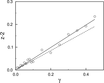
Figure 6: Shown are simulation results for the scaling exponent for the case $n=0$, $\mu=\lambda$, and $\beta=4$ when torsion is included. The error bars are given roughly by the scatter in the data. The best linear fit to the simulation data is shown (solid line). Also shown (dashed line) is the prediction assuming that the other parameters do not flow, $z=2+4\gamma/(3\pi)$.

There appears to be relatively little if any renormalization of $z$ away from the bare value. A power law behavior of the long-time mean square displacement in the presence of torsion is observed, although localization at exceptionally long times still cannot be ruled out.

It is clear that within the continuum assumption of the diffusion equation, the torsion term affects the dynamics. The contribution to the diffusion coefficient is explicit in eq. (51) for the case $n>0$. For $n=0$, the results shown in Fig. 6 differ from those without torsion in Fig.  5. Note that the results with torsion, as those without torsion, differ substantially from the approximate results of Bausch et al. (1994); Krukowski and Turski (1993), noticeably through their dependence on the two Lamé coefficients.

VIII Conclusion

We have given a treatment of the effect of topological disorder on transport properties. Within the lattice reconstruction predicted by linear elasticity theory, topological disorder is manifestly different from charged, potential-type disorder. The net effect of the defects, through local lattice expansion and contraction and global topological rearrangement of lattice connectivity, is an overall reduction of the transport. Interestingly, randomly placed dislocations, or randomly placed disclinations with no net disclinicity, lead to anomalous subdiffusive behavior when the displacement fields of linear elasticity are used.

References

Bouchaud and Georges (1990)
J. P. Bouchaud and
A. Georges,
Phys. Rep. 195,
127 (1990).
Nelson (1983)
D. R. Nelson,
Phys. Rev. B 27,
2902 (1983).
Rubinstein et al. (1983)
M. Rubinstein,
B. Shraiman, and
D. R. Nelson,
Phys. Rev. B 27,
1800 (1983).
Cha and Fertig (1995)
M.-C. Cha and
H. A. Fertig,
Phys. Rev. Lett. 74,
4867 (1995).
Park and Deem (1998a)
J.-M. Park and
M. W. Deem,
Phys. Rev. E 58,
1487 (1998a).
Bausch et al. (1994)
R. Bausch,
R. Schmitz, and
L. A. Turski,
Phys. Rev. Lett. 73,
2382 (1994).
Krukowski and Turski (1993)
S. Krukowski and
L. A. Turski,
Phys. Lett. A 175,
349 (1993).
Kleinert and Shabanov (1998)
H. Kleinert and
S. V. Shabanov,
J. Phys. A 31,
7005 (1998).
Ikeda and Watanabe (1989)
N. Ikeda and
S. Watanabe,
Stochastic Differential Equations and Diffusion
Processes (Elsevier, Amsterdam,
1989), pp. 281, 285.
Seung and Nelson (1988)
S. Seung and
D. R. Nelson,
Phys. Rev. A 38,
1005 (1988).
Kreyszig (1991)
E. Kreyszig,
Differential Geometry (Dover
Publications, New York, 1991),
the matrix of Eq. (5) is, moreover, nothing
more than the inverse of the metric tensor of differential geometry.
Lee (1994)
B. P. Lee, J.
Phys. A 27, 2633
(1994).
Lee and Cardy (1995)
B. P. Lee and
J. Cardy, J.
Stat. Phys. 80, 971
(1995); 87, 951 (1997).
Kravtsov et al. (1985)
V. E. Kravtsov,
I. V. Lerner,
and V. I.
Yudson, J. Phys. A
18, L703 (1985).
Park and Deem (1998b)
J.-M. Park and
M. W. Deem,
Phys. Rev. E 57,
3618 (1998b).
Nabarro (1987)
F. R. N. Nabarro,
Theory of Crystal Dislocations
(Dover Publications, New York,
1987).
Zinn-Justin (1996)
J. Zinn-Justin,
Quantum Field Theory and Critical Phenomena
(Clarendon Press, Oxford,
1996), 3rd ed.
Pham and Deem (1998)
V. Pham and
M. W. Deem,
J. Phys. A: Math. Gen. 31,
7235 (1998).