Calculation of nanowire thermal conductivity using complete phonon dispersion relations

Abstract

The lattice thermal conductivity of crystalline Si nanowires is calculated. The calculation uses complete phonon dispersions, and does not require any externally imposed frequency cutoffs. No adjustment to nanowire thermal conductivity measurements is required. Good agreement with experimental results for nanowires wider than 35 nm is obtained. A formulation in terms of the transmission function is given. Also, the use of a simpler, nondispersive ”Callaway formula”, is discussed from the complete dispersions perspective.

Determining the thermal conductivity of semiconducting nanowires plays a crucial role in the development of a new generation of thermoelectric materials Mahan . However, experimental results are still scarce Fon . The first measurements of the thermal conductivity of Si nanowires in the $\sim 20-115nm$ range have been recently reported in ref.Li, . From a theoretical point of view, it is important to be able to quantitatively calculate lattice thermal conductivities of nanowires in a predictive fashion. In the past, several techniques have become widespread in the calculation of thermal conductivities of bulk materials Callaway ; Holland ; Parrott ; Berman . These works are based on linearized dispersion models that involve a certain number of adjustable parameters. In principle, one might hope that a proper account of the boundary scattering in the nanowires might enable us to predict nanowire thermal conductivities using the procedures of ref. Callaway, or ref. Holland, , without any parameters other than those obtained from fitting the bulk data. Nevertheless, calculations using those two approaches did not yield reasonable results for nanowires APL . A first goal of this paper is to show that, using accurate phonon dispersion relations, predictive calculations of the nanowire thermal conductivities can be done, which do not involve any adjustable parameter to fit the nanowire experimental curves. A second result in this paper shows that the use of a ”modified” Callaway approach is still possible for nanowires, although this second approach is not predictive, and requires adjustment to nanowire measurements.

For a nanowire suspended between two thermal reservoirs, its thermal conductance, $\sigma(T)$, is defined as the flow of heat current through the wire when a small temperature difference $\Delta T$ exists between the reservoirs, divided by $\Delta T$ and taking the limit $\Delta T\rightarrow 0$. If the phonons transmit ballistically, the conductance is

$$\sigma_{b}(T)=\sum_{\alpha}\int_{0}^{\pi/a_{z}}{dk_{z}\over 2\pi}[\hbar\omega v_{z}(\alpha,k_{z}){df_{B}\over dT}]$$ (1)

where $\alpha$ is a set of discrete quantum numbers labeling the particular subbands in the one dimensional phonon dispersion relations. $f_{B}$ is the Bose distribution, and $v_{z}$ is the speed of the phonon in the axial direction of the nanowire, $z$. Using $v_{z}dk_{z}=d\omega$ we have Rego

$$\sigma_{b}(T)=\sum_{\alpha}\int_{\omega^{i}_{\alpha}}^{\omega^{f}_{\alpha}}{d\omega\over 2\pi}[\hbar\omega{df_{B}\over dT}]\equiv\int_{0}^{\infty}\Xi_{b}(\omega){\hbar\omega\over 2\pi}{df_{B}\over dT}d\omega$$ (2)

where $\omega^{i(f)}_{\alpha}$ is the lower (upper) frequency limit of subband $\alpha$. Here we have defined the ballistic transmission function, $\Xi_{b}(\omega)$, which simply corresponds to the number of phonon subbands crossing frequency $\omega$.

However, in general, phonon scattering takes place in the wire and at the contacts, so that the transmission function is not given by the simple mode count stated above. In general, the transmission function can be obtained from the Green function of the system. This allows to study the interesting issues of ballistic versus diffusive transport deJong , or the effect of one dimensional localization.Beenakker We shall not be concerned with those phenomena here, but shall assume that diffusive transport takes place and the Boltzmann transport equation is valid. From this standpoint, it has been shown that a mode’s transmission can be described in terms of a characteristic relaxation length in the wire’s direction, $\lambda_{\alpha}(\omega)$, such that $\sigma_{diff}(T)\simeq\sum_{\alpha}\int{\lambda_{\alpha}(k_{z})\over L}{\hbar\omega_{\alpha}(k_{z})\over 2\pi}{df_{B}\over dT}v_{z}(\alpha,k_{z})dk_{z}$ where $L$ is the nanowire’s length Klemens . The thermal conductivity is defined as $\kappa(T)={L\over s}\sigma$, where $s$ is the cross section of the nanowire. Therefore, in this diffusive regime

$$\kappa(T)={1\over s}\sum_{\alpha}\int_{0}^{\pi/a_{z}}\lambda_{\alpha}(k_{z}){\hbar\omega_{\alpha}(k_{z})\over 2\pi}{df_{B}\over dT}v_{z}(\alpha,k_{z})dk_{z}.$$ (3)

To obtain the thermal conductivity we must compute the complete dispersion relations for the wire, $\omega_{\alpha}(k_{z})$, which, using $v_{z}(\alpha,k_{z})={d\omega_{\alpha}(k_{z})\over dk_{z}}$, allows us to express the previous equation as

$$\kappa(T)={1\over s}\int_{0}^{\infty}(\sum_{\alpha}\lambda_{\alpha}(\omega)){\hbar\omega\over 2\pi}{df_{B}\over dT}d\omega,$$ (4)

$$\hbox{with }\ \lambda_{\alpha}(\omega)\equiv\left\{\matrix{\lambda_{\alpha}(k_{z}(\alpha,\omega)),&\omega_{\alpha}^{i}<\omega<\omega_{\alpha}^{f}\cr 0,&\hbox{otherwise.}\cr}\right.$$ (5)

If the modes’ lifetimes $\tau(\omega)$ are independent of the subband, and only depend on the frequency, then, the relaxation lengths are given by

$$\lambda_{\alpha}(\omega)=v_{z}(\alpha,\omega)\tau(\omega), \omega_{\alpha}^{i}<\omega<\omega_{\alpha}^{f}$$ (6)

Knowing $\omega_{\alpha}(k_{z})$ and $\tau(\omega)$, Eqs. (4-6) already allow us to compute the thermal conductivity. Nevertheless, it is useful to recast Eq. (4) into an equivalent form, so as to explicitly retain the ”transmission function” concept. For this, we define $N_{b}(\omega)$ as the number of phonon subbands crossing frequency $\omega$:

$$N_{b}(\omega)\equiv\sum_{\alpha}\Theta(\omega-\omega_{\alpha}^{i})\Theta(\omega_{\alpha}^{f}-\omega),$$ (7)

$$\Theta(x)=\left\{\matrix{1&x\geq 0\cr 0&x<0.\cr}\right.$$ (8)

The average group velocity in the axial direction is defined as

$$\langle v_{z}(\omega)\rangle\equiv\left(\sum_{\alpha}v_{z}(\alpha,\omega)\right)/N_{b}(\omega)$$ (9)

where the sum extends to subbands $\alpha$ such that $\omega_{\alpha}^{i}<\omega<\omega_{\alpha}^{f}$. From Eqs. (5-6) and (9), it follows that $\sum_{\alpha}\lambda_{\alpha}(\omega)=\tau(\omega)\sum_{\alpha}v_{z}(\alpha,\omega)=\tau(\omega)N_{b}(\omega)\langle v_{z}(\omega)\rangle$. Thus Eq. (4) can be recast into its completely equivalent form

$$\kappa(T)={L\over s}\int_{0}^{\infty}\Xi(\omega){\hbar\omega\over 2\pi}{df_{B}\over dT}d\omega$$ (10)

$$\hbox{with }\ \ {L\over s}\Xi(\omega)=\tilde{N}_{b}(\omega)\tau(\omega)\langle v_{z}(\omega)\rangle.$$ (11)

Here, the diffusive transmission function $\Xi$ has been defined, and

$$\tilde{N}_{b}(\omega)\equiv N_{b}(\omega)/s.$$ (12)

Computation of the transmission function requires the obtention of the full phonon dispersions for the nanowire. We now proceed to separately study each of the three factors in Eq. (11): $\tilde{N}_{b}(\omega)$, $\tau(\omega)$, and $\langle v_{z}(\omega)\rangle$.

$\tilde{N}_{b}(\omega)$ is obtained from the complete dispersion relations for the wire. To compute them, we have used the interatomic potential proposed by ref. Harrison, , in which the energy of the system is given as the sum of two and three body terms. The two body terms are defined as

$$\delta E_{0}(i,j)=\hbox{${1\over 2}$ }C_{0}{(d_{i,j}-d_{0})^{2}/d_{0}^{2}}$$

for every pair of nearest neighbors $i$ and $j$, where $d_{i,j}$ is the distance between the atoms and $d_{0}$ is the lattice equilibrium distance. The three body terms are defined as

$$\delta E_{1}(i,j,k)=\hbox{${1\over 2}$ }C_{1}\delta\Theta_{i,j,k}^{2}$$

for every pair of bonds joining atoms $i$, $j$ and $k$, where $\delta\Theta$ is the deviation with respect to the equilibrium angle between the two bonds in the lattice. The constants are $C_{0}=49.1eV$ and $C_{1}=1.07eV$ Harrison . With this potential the dynamical matrix of the system is constructed, and the dispersion relations for the wire are calculated. The inset of fig. 1 shows one example. The bulk dispersions obtained with the Harrison potential are close to those experimentally measured. Although a more sophisticated calculation of the interatomic potential is possible using ab initio techniques, this would only result in minor differences in the calculated $\tilde{N}_{b}$ and the conductivities computed from it.

The dispersions in general depend on the cross sectional shape of the wire, and on whether its surface is reconstructed or not, clean or coated by an overlayer, etc. As the surface/volume ratio decreases, these differences become smaller, and for wide enough wires of cross section $s$, the function $\tilde{N}_{b}(\omega)\equiv N_{b}(\omega)/s$ approaches a limiting form, $\tilde{N}_{b}^{\infty}(\omega)$, independent of the surface features. To ascertain whether it is valid to approximate $\tilde{N}_{b}(\omega)$ by $\tilde{N}_{b}^{\infty}(\omega)$ for nanowires wider than 35 nm, the former was calculated for nanowires of increasing width, with frozen boundary conditions. (As compared to ”free boundary”, frozen boundary conditions are more similar to the experimental situation, where 1 nm of $SiO_{2}$ coats the wire.) For a romboidal cross section wire of 17 nm side, $\tilde{N}_{b}$ deviates from the limiting value $\tilde{N}_{b}^{\infty}$ by less than $0.1\%$. Therefore, for the widths considered here ($l>35nm$), $\tilde{N}_{b}=\tilde{N}_{b}^{\infty}$ is a valid assumption. In the thermal conductivity calculations presented here, $\tilde{N}_{b}^{\infty}$ for the 110 direction was used (fig. 1).

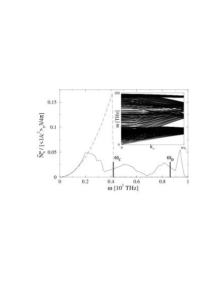
Figure 1: Solid line: function $\tilde{N}_{b}^{\infty}(\omega)$ for the (110) direction, calculated using complete phonon dispersions. Dotted line: parabolic approximation to $\tilde{N}_{b}^{\infty}(\omega)$, for a non dispersive medium. Inset: dispersion relations for a 2.2 nm wide wire with frozen boundary.

The phonon lifetime is commonly given by Matheissen’s rule, expressing the total inverse lifetime as the sum of the inverse lifetimes corresponding to each scattering mechanism. For bulk or a macroscopically thick whisker, the expressions used for boundary, anharmonic and impurity scattering are Asen-Palmer :

$$\tau^{-1}_{b}= (\langle 1/c\rangle_{b}lF)^{-1}$$

$$\tau_{a}^{-1}= BT\omega^{2}e^{-C/T}$$ (13)

$$\tau^{-1}_{i}= A\omega^{4}$$

From here on, $\langle\rangle_{b}$ denotes averaging in the three acoustic branches, i.e. $\langle 1/c\rangle_{b}\equiv{1\over 3}\sum_{i=1}^{3}1/c_{i}$, where $c_{i}$ is the speed of sound for each branch. (Do not confuse with averages over subbands, denoted by $\langle\rangle$.) A, B and C are numerical constants specified later. $l$ is the wire’s lateral dimension, and $F$ relates the boundary scattering rate to the shape and specularity of the sample’s boundary. Eqs. (13) are always valid for wire thicknesses larger than a certain threshold, $L_{3D}$. On the other hand, if the width of the whisker is very small, such that $L<<L_{3D}$, the frequency difference between consecutive phonon subbands gets large. This confinement modifies the inter-subband scattering, and the validity of Eqs. (13) breaks down. A criterion to estimate $L_{3D}$ is: confinement is important if the energy spacings between consecutive subbands, $\hbar\Delta\omega$, are larger or comparable to the thermal energy $k_{B}T$. The largest intersubband spacings are of the order of $\hbar\Delta\omega\sim{2\pi\over l}\hbar c$. Thus, for Eqs. 13 to be valid at temperatures $40^{o}K$ or higher, we need $l>10nm$. This is well fulfilled for nanowires in the 37-115 nm range, as the ones experimentally measured Li . Therefore, for these widths, we use Eqs. 13 without modification. The good agreement with experimental results corroborates their validity. For sub 20 nm widths, confinement effects may be expected.

Anharmonic scattering should include the effects of umklapp as well as normal processes. In some works normal processes have been omitted in favor of umklapp scattering, without extensive discussion Fon ; Balandin . In general, if resistive processes dominate, the normal relaxation time can be disregarded Klemens . For the higher frequencies, umklapp scattering is proportional to $\omega^{2}$, and it thus dominates over normal processes, which depend linearly on frequency HanKlemens . At the lower frequencies, in the case of nanowires, boundary scattering dominates. This justifies the form of $\tau_{a}$ in Eq. 13, which is the functional dependence for umklapp scattering at the higher frequencies. Constants B and C were adjusted to reproduce the bulk material’s experimental thermal conductivity curve, yielding $B=1.73\times 10^{-19}s/K$ and $C=137.3K$. Parameter $A=1.32\times 10^{-45}s^{3}$ is analytically determined from the isotope concentration, and it should not be adjusted Asen-Palmer , so we maintain the value given in [Holland, ].

The third term in Eq. (11), $\langle v_{z}(\omega)\rangle$, is also calculated from the dispersion relations. In a frozen boundary wire, it is a matter of simple geometry to prove that at the lower part of the spectrum,

$$\langle v_{z}\rangle\simeq{2\over 3}\langle 1/c\rangle_{b}/\langle 1/c^{2}\rangle_{b}$$ (14)

where $\langle 1/c^{2}\rangle_{b}\equiv{1\over 3}\sum_{i=1}^{3}1/c^{2}_{i}$. The relaxation times, Eq. (13) are quite rough, since they only depend on the lower spectrum speeds of sound. Thus, no additional approximation is incurred if Eq. (14) is used for the third term in Eq. (11).

Fig. 2 shows the results of the calculation using the complete dispersions transmission function into Eq. (10). Calculations for nanowires of diameters $Fl=38.85$, $72.8$ and $132.25$ nm are shown, together with experimental results from ref. Li, . Although the TEM measured diameters of the experimental nanowires were 37, 56 and 115 nm, variations in cross sectional shape, as well as thickness of the nanowire’s oxide surrounding layer are possible, so that the cross sectional area is not accurately known. Assuming $l$ equal to the TEM diameters, values can be assigned to $F$, which in the current case are $F\simeq 1.05$, $1.3$ and $1.15$. These values suggest that the boundary scattering is very diffusive, rather than specular.

Figure 2: Thermal conductivities versus temperature calculated using the complete dispersions transmission function, for $Fl=1.05\times 37nm$ (solid), $1.3\times 56nm$ (dotted) and $1.15\times 115nm$ (dashed). Dots: experimental results from ref. Li, . Inset: bulk.

Let us see what would happen if, instead of the atomistically calculated complete dispersions, a nondispersive medium were used. In such a case, for frozen boundary, function $\tilde{N}_{b}^{\infty}(\omega)$ is analytical, having a parabolic dependence:

$$\hbox{(non dispersive)}\ \ \tilde{N}_{b}^{\infty}(\omega)\simeq \sum_{i=1}^{3}\int_{0}^{\omega/c_{i}}2\pi k_{\perp}{dk_{\perp}\over(2\pi)^{2}}$$

$$= {3\over 4\pi}\omega^{2}\langle 1/c^{2}\rangle_{b}$$ (15)

Substituting Eq. (15) into Eqs. (10) and (11), the Callaway formula Callaway ; Holland is obtained. Since now the subbands extend to infinite frequency, an upper cutoff has to be imposed, which was not necessary when using the complete dispersions, because for these ones the upper bands’ limits are well defined. Traditionally, the Debye frequency, $\omega_{D}$ (86 THz for Si), has been used as cutoff Callaway . If we do this, the calculated thermal conductivities for nanowires are in large disagreement with experimental measurements. As fig. 3(a) shows, no calculated curve agrees in shape with any experimental curve: the theoretical inflection points are always too high. Comparison of the parabolic approximation to $\tilde{N}_{b}^{\infty}$ (Eq. 15) with the correct $\tilde{N}_{b}^{\infty}$, in fig. 1, shows that the former grossly overestimates the transmission of the high frequency phonons, if its cutoff is set at $\omega_{D}$. Nevertheless, if a lower cutoff $\omega_{C}$ is chosen, the ”Callaway” and ”correct” $\tilde{N}_{b}^{\infty}(\omega)$ curves are more similar. Using $\omega_{C}$, the shapes of the theoretical thermal conductivity curves agree well with the experimental ones (fig. 3(b)). The values of the lifetime parameters B and C are those that yield the correct bulk limit: $3.9\times 10^{-19}s/K$ and $223.1^{o}K$ for fig. 3(a), and $1.7\times 10^{-19}s/K$ and $151.8^{o}K$ for fig. 3(b).

For bulk, it is possible to obtain a good fit of experimental data using either $\omega_{C}$ or $\omega_{D}$ (see inset of fig. 3), because the dominant umklapp scattering makes the role of high frequencies less important. For nanowires, boundary scattering dominates, and high frequencies play a more important role. Therefore, using the experimental Debye frequency as a cutoff for the Callaway formula does not yield correct results for nanowires, although good results can be obtained with a lower, adjusted cutoff. This one must be determined by comparison with nanowire experimental results (non predictive approach). On the other hand, if the atomistically calculated, complete dispersion relations are used, good agreement with experimental results is obtained (fig. 2), with no need for prior knowledge of any experimental measurements for nanowires.

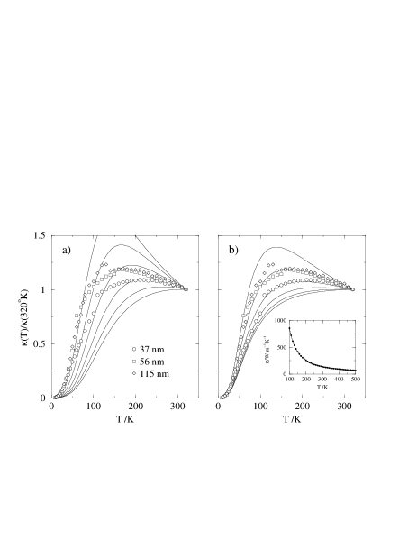
Figure 3: Thermal conductivity normalized by its value at $320^{o}K$, for nanowires of different widths, calculated by the Callaway formula with cutoff at $\omega_{D}$ (86 THz) (a), and at $\omega_{C}$ (42 THz) (b). (Experimental results from ref. Li, .) Inset: bulk thermal conductivity for the two cases (overlapping almost completely) and experimental curve from ref. Holland, (dots).

To conclude, it was shown that, by using complete, atomistically computed phonon dispersions, it is possible to predictively calculate lattice thermal conductivity curves for nanowires, in good agreement with experiments. On the other hand, it was not possible to obtain correct results with the approximated Callaway formula. Still, good results could be obtained with a modified Callaway formula, although non predictively. The results of this paper are only expected to apply to ”nanowhiskers” for which phonon confinement effects are unimportant. Si nanowires wider than $\sim 35nm$ are within this category.

I am indebted to D. Li, A. Majumdar and Ph. Kim for communication of their experimental data, and discussions, and to A. Balandin and Liu Yang for discussions.

References

- (1) G. Mahan, B. Sales and J. Sharp, Physics Today, March 1997, p.42.
- (2) W. Fon, K. C. Schwab, J. M. Worlock and M. L. Roukes, Phys. Rev. B 66, 045302 (2002).
- (3) D. Li, Y. Wu, P. Kim, L. Shi, P. Yang and A. Majumdar, Appl. Phys. Lett., in press.
- (4) J. Callaway, Phys. Rev. 113, 1046 (1959).
- (5) M. G. Holland, Phys. Rev. 132, 2461 (1963).
- (6) J. E. Parrott and A. D. Stuckes, Thermal conductivity of solids, Pion Ltd., London (1975).
- (7) R. Berman, Thermal conductivity of solids, Clarendon Press, Oxford (1976).
- (8) N. Mingo, L. Yang, D. Li, and A. Majumdar, to be published.
- (9) For a nondispersive medium see L. G. C. Rego and G. Kirczenow, Phys. Rev. Lett. 81, 232 (1998), or D. H. Santamore and M. C. Cross, Phys. Rev. B 63, 184306 (2001).
- (10) M. J. M. de Jong, Phys. Rev. B 49, 7778 (1994).
- (11) C. W. J. Beenakker, Rev. Mod. Phys. 69, 731 (1997).
- (12) P. G. Klemens, in Solid State Physics, edited by F. Seitz and D. Turnbull (Academic, New York, 1958), Vol. 7, p.1.
- (13) W. A. Harrison, Electronic Structure and the Properties of Solids, Dover (1989).
- (14) J. Zou and A. Balandin, J. Appl. Phys. 89, 2932 (2001).
- (15) M. Asen-Palmer, K. Bartkowski, E. Gmelin, M. Cardona, A. P. Zhernov, A. V. Inyushkin, A. Taldenkov, V. I. Ozhogin, K. M. Itoh and E. E. Haller, Phys. Rev. B 56, 9431 (1997).
- (16) A. Balandin and K. Wang, Phys. Rev. B 58, 1544 (1998).
- (17) Y. -J. Han and P. G. Klemens, Phys. Rev. B 48, 6033 (1993).
- (18) Yong-Jin Han, Phys. Rev. B 54, 8977 (1996).