The Role of Friction in Compaction and Segregation of Granular Materials

Abstract

We investigate the role of friction in compaction and segregation of granular materials by combining Edwards’ thermodynamic hypothesis with a simple mechanical model and mean-field based geometrical calculations. Systems of single species with large friction coefficients are found to compact less. Binary mixtures of grains differing in frictional properties are found to segregate at high compactivities, in contrary to granular mixtures differing in size, which segregate at low compactivities. A phase diagram for segregation vs. friction coefficients of the two species is generated. Finally, the characteristics of segregation are related directly to the volume fraction without the explicit use of the yet unclear notion of compactivity.

I Introduction:

Friction plays a significant role in packings of grains in a granular material, however due to the non-equilibrium nature of such materials their macroscopic properties do not trivially result from the microscopic physics of their constitutes. Compaction and segregation are two macroscopic phenomena which occur in granular materials undergoing series of extensive operations edwards_oakeshott_physica_a_1989 (operations of a statistical nature rather than “Maxwell-demon” operations which act on single grains). Packings of identical hard spheres compacted by extensive operations reach a state of random close packing (RCP), rather than an ordered crystalline packing, which has a higher volume fraction (defined as the ratio of the sum of grain volumes to the volume the system occupies). Understanding the process leading to RCP, its geometrical properties and whether higher volume fractions may be obtained is of great importance for physics and for engineering. The tendency towards segregation in granular mixtures comprised of grains with various mechanical properties is interesting for the physicist and disturbing for the engineer, for whom a homogeneous mixture is often an industrial need (for a review see kaye ).

Segregation in granular materials has received much attention in recent years (for a review see ristow ). The phenomenon is observed for grains varying in size cantelaube_1995 , shape lawrence_1968 , friction coefficient zik_1994 and density shinbrot_1998 . Segregation occurs due to vibration cooke_1996 , tapping knight_1993 , rotation zik_1994 , pouring makse_nature_1997 and shearing williams_1976 . Experiments are performed for mixtures of many particles of two different species (for a review see ottino_2000 ) and with single intruder particles in systems of a single species clement_1995 . Existing theoretical modeling of segregation due to rotation zik_1994 ; levine_chaos_1999 ; lai_1997 and to pouring makse_nature_1997 ; boutreux_de_gennes_1996 is based on kinetic phenomena: segregation is explained as a result of different flow properties of the different species. Monte Carlo simulations of dynamic phenomena in vibrated systems give insight into segregation rosato_1987 as well as compaction dynamics of single species systems mehta_barker_1991 . Similar dynamic phenomena have been captured analytically in models based on free volume considerations boutreux_de_gennes_1997 ; ben_naim_1998 ; nowak_1998 .

This paper deals with the role of friction in compaction and segregation through the analysis of the static properties of granular materials. The results obtained may be used in order to verify experimentally the validity of such models. One such proposal for the description of static granular materials is the analogy to the statistical mechanics of thermodynamic of Edwards edwards_oakeshott_physica_a_1989 , a more detailed description of which will be given in the following section. The central idea behind it is that even though the system is static and does not move with time within the ensemble of mechanically stable arrangement of the grains, we may assume ergodicity and employ statistical mechanics considerations for the probability of finding the system in any one of its states. This model requires the existence of an analog of temperature, referred to as “compactivity” (Other effective temperatures may be defined for jammed granular materials langer_liu_2000 ; ono_liu_2002 , and attempts have been done to connect them to the compactivity barrat_2000 ; makse_nature_2002 ). Recent experimental evidence for reversibility in compaction processes nowak_1997 has provided justification for this thermodynamic analogy and have proposed a connection between compactivity and experimentally controllable quantities edwards_grinev_PRE_1998 , however the proposal remains controversial.

Edwards’ hypothesis is that an analog of the free energy $Y=V-XS$ is minimized where $V$ is the system volume, $S$ is the entropy and $X$ is the compactivity. Our expectation that this formalism may predict frictional segregation is based on the following argument. Consider two systems of identical grains, such that the friction coefficient of the first system, $\mu_{1}$, is greater than that of the second system, $\mu_{2}$. Then $S_{1}>S_{2}$ because every configuration available to the second system may be identically realized to the first system, while the converse is not true. This suggests that under certain circumstances a mixture of grains with different friction coefficients may prefer to segregate in order that its entropy be maximized, competing with the preference of the entropy of mixing to be maximized in the homogeneously mixed state.

The statistical hypothesis has been used to investigate segregation in binary mixtures of species differing in size by mapping them to the Ising model, resulting in segregation below some critical compactivity edwards_oakeshott_physica_a_1989 ; mehta_edwards_physica_a_1989 . Recent geometrical calculations have enabled relating the ideas of the statistical proposal to actual densities of granular systems blumenfeld_2003 .

In section II we use Edwards’ statistical hypothesis together with a simple mechanical model for the quantitative description of friction in 2D and 3D single species granular materials. This is combined with simple calculations of Voronoi cell volumes for general coordination numbers resulting in the dependence of volume fraction on friction coefficient and compactivity. Section III uses the mean-field approximation in order to describe segregation in a binary mixture of grains differing in frictional properties. Unlike mixtures of grains differing in size, which may be mapped to the Ising model edwards_oakeshott_physica_a_1989 ; mehta_edwards_physica_a_1989 , frictional differences between grains result in larger entropy for the rougher grains. Therefore, these systems may not be mapped exactly onto the Ising model and segregation occurs above a critical compactivity and not below it. We then generate a phase diagram for segregation vs. friction coefficients of the two species. Finally, the dependence of the results on compactivity is eliminated by using the volume fraction as a measure for compactivity. Section IV concludes with a summary of the results.

II Single Species:

II.1 Statistical Model

We use the statistical mechanics hypothesis proposed by Edwards edwards_oakeshott_physica_a_1989 for the description of jammed granular systems. In this formalism each mechanically stable arrangement of the grains is equivalent to a micro-state in statistical mechanics, and the total volume the grains occupy plays the role of the energy. The analog of temperature is assumed to exist, is denoted X and is called the compactivity. We measure X in units of volume so that the analog of the Boltzman constant is equal to unity. In analogy with the canonical ensemble of states in thermal systems, the probability for the occurrence of a state with volume V is assumed to be proportional to $e^{-V/X}$.

We consider a system of N identical spherical (in 3D) or circular (in 2D) grains. For every arrangement of the grains, the total volume of the system may be written as the sum over all grains of the Voronoi cell volume around each grain, $v_{i}$:

$$V=\sum^{N}_{i=1}v_{i}.$$ (1)

Average volumes of Voronoi cells, calculated neglecting spatial correlations between locations of grains, have been shown to agree with exact calculations richard_2001 . Moreover, correlations have been shown to have a small effect on the dependence of total volume on compactivity blumenfeld_2003 . Therefore, we use a mean-field approximation and assume the volume of every Voronoi cell is evenly distributed between a minimal and maximal volume, $v_{min}$ and $v_{max}$. The geometrical and mechanical considerations determining these volumes will be presented in the following section, and at this stage it is only assumed $v_{min}$ and $v_{max}$ are uniform for all grains in the system.

Following the analogy with the canonical ensemble, we may calculate the pseudo partition function:

$$Z = \int^{v_{max}}_{v_{min}}\cdot\cdot\cdot\int^{v_{max}}_{v_{min}}e^{-\sum v_{i}/X}dv_{1}\cdot\cdot\cdot dv_{N}=$$ (2)

$$= \left(\int^{v_{max}}_{v_{min}}e^{-v/X}dv\right)^{N}=$$

$$= \left(2X\cdot e^{-v_{mid}/X}\cdot\sinh\left(\frac{\Delta v}{X}\right)\right)^{N},$$

where we have introduced the notations, $v_{mid}\equiv(v_{min}+v_{max})/2$ and $\Delta v\equiv(v_{max}-v_{min})/2$.

The average volume per grain may easily be derived from the partition function as:

$$<v> = \frac{<V>}{N}=\frac{1}{N}X^{2}\frac{\partial\ln(Z)}{\partial X}=$$ (3)

$$= v_{mid}+X-\Delta v\cdot\coth\left(\frac{\Delta v}{X}\right).$$

This expression has been derived in edwards_oakeshott_physica_a_1989 , and it is clearly seen that as $X\rightarrow 0$, $<v>\rightarrow v_{min}$ and as $X\rightarrow\infty$, $<v>\rightarrow v_{mid}$. This is analogous to thermal systems, where at low temperatures the system is most probable to be found in its ground state, and as the temperature is increased exited states are occupied with increasing probability until the limit of infinite temperature, where all states are occupied with an equal probability, and the system’s energy is the average energy of all these states.

II.2 Mechanical Model

We would now like to introduce mechanical and geometrical considerations to estimate $v_{min}$ and $v_{max}$, which must be known in order to evaluate the expression in eq. (3). The minimal volume is achieved for hexagonal packing in 2D and face centered cubic or hexagonal close packing in 3D. The corresponding Voronoi cell volumes are $v_{min}^{2D}=\sqrt{12}r^{2}$ and $v_{min}^{3D}=\sqrt{32}r^{3}$, where r is the grain radius. The resulting volume fractions are $\Phi_{max}^{2D}={\pi r^{2}}/{v_{min}^{2D}}={\pi}/{\sqrt{12}}\simeq 0.91$ and $\Phi_{max}^{3D}={\frac{4\pi}{3}r^{3}}/{v_{min}^{3D}}={\pi}/{\sqrt{18}}\simeq 0.74$.

Although purely geometric considerations determine $v_{min}$, the frictional forces between the grains manifest themselves in $v_{max}$. The idea behind this is that friction at grain contacts allows for the formation of arcs and for a gradual decrease in the number of contacts per grain silbert_2002 , which in turn increases the volume of the Voronoi cell around every grain.

In order to estimate the effect of friction in granular materials we will consider “toy-systems” consisting of a small number of grains (three in 2D and four in 3D), calculate the effect of friction there, and use the result in order to obtain an approximate prediction for the dependence of $v_{max}$ on the friction coefficient, $\mu$. This, in turn, may be inserted together with $v_{min}$ into eq. (3) in order to obtain an approximate expression for the dependence of the total volume of the system, and hence of the volume fraction, on $\mu$. The results will depend on the compactivity, whose physical significance still requires elucidation. However, even without understanding its significance, a few predictions for experimental results may be drawn from the model presented here.

The 2D “toy-system” consists of two grains lying on top of a horizontal plane and a third grain lying on top of these (see fig. 1). All grains and the horizontal plane are assumed to be hard, and frictional forces with an equal coefficient of friction, $\mu$, act at all four contacts. A uniform gravitational force acts downwards on all grains. The condition for mechanical equilibrium is that forces and torques acting on all grains vanish. It can easily be seen that this is satisfied whenever:

$$\frac{\sin\theta}{1+\cos\theta}\leq\mu,$$ (4)

where $\theta$ is half the angle between contacts of the top grain with the bottom grains (see fig. 1). For $\mu\geq 1$ eq. (4) is always satisfied, and any state with ${\pi}/{6}\leq\theta\leq{\pi}/{2}$ is mechanically stable. For smaller values of $\mu$ only states with $\theta\leq\theta_{max}$ are mechanically stable, where $\theta_{max}$ is determined from

$$\frac{\sin\theta_{max}}{1+\cos\theta_{max}}=\mu.$$ (5)

If $\mu\leq(2+\sqrt{3})^{-1}\simeq 0.3$, the frictional forces cannot hold the top grain on top of the two bottom ones, and these simple considerations may not be used in order to determine $v_{max}$. In this case the volume of the Voronoi cell around every grain is set in the model to $v_{min}$. Substituting this into eq. (3) yields $<v>=v_{min}$, which corresponds to the maximal volume fraction quoted earlier, and hence, to crystallization. Therefore, this model may not be used for frictionless systems, since it predicts crystallization at every compactivity.

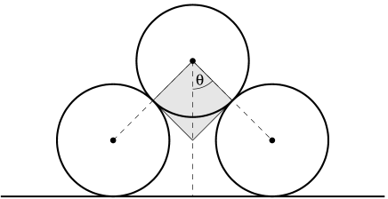
Figure 1: The 2D “toy-system”. The shaded rhombus is the segment of the Voronoi cell lying between two adjacent contacts.

In 3D we consider three grains in an equilateral triangle lying on top of a horizontal plane and a fourth grain lying on top of them (see fig. 2a). As in the 2D case, all grains and the horizontal plane are assumed to be hard, frictional forces with an equal coefficient of friction, $\mu$, act at all six contacts, and a uniform gravitational force acts downwards on all grains. Again, the condition for mechanical equilibrium can easily be seen to be given by eq. (4), however now $\theta$ is the angle between the vertical direction and the line connecting the top grain with any one of the bottom grains (see fig. 2b). As in 2D, for small values of $\mu$, and specifically for frictionless systems, these considerations cannot be used to estimate the volume fraction, since this model predicts crystallization regardless of compactivity, while actual 3D granular systems do not fully crystallize, but fall into an RCP state.

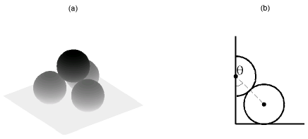
Figure 2: a) The 3D “toy-system”. b) Section of the top grain and one of the bottom grains.

We would now like to use the results of these simple considerations to evaluate the maximal volume of the Voronoi cell around every grain in a granular material. In such systems frictional forces allow the existence of large angles between contacts of every grain with its surrounding grains. We assume that the maximal angle between contacts in a granular material depends on the friction coefficient in a similar manner to its dependence in the toy-systems. Moreover, in order to calculate the Voronoi cell volume around every grain we assume the angles between adjacent contacts of this grain with its surrounding grains are uniform and are given by $\theta$ as in the toy-systems. Note that since we allow $\theta$ to vary continuously, it may not necessarily be physically possible to build these packings, even locally. In 2D it is possible only if $\theta$ is an integer fraction of $\pi$, while in 3D it is possible only if the coordination number is 4 or 6, which correspond to $\theta\simeq 1.23$ and $\theta\simeq 0.96$, respectively. The general expression for the Voronoi cell volume is (see appendix A):

$$v(\theta)=\left\{\begin{array}[]{cc}\frac{\pi r^{2}\tan\theta}{\theta}&\mbox{(2D)}\\ \frac{\pi r^{3}\sqrt{3}\sin\theta\tan\theta}{(1+3\cos^{2}\theta)\tan^{-1}(\sqrt{\tan\frac{3\alpha}{4}\tan^{3}\frac{\alpha}{4}})}&\mbox{(3D)}\end{array}\right.,$$ (8)

where $\alpha=\cos^{-1}((3\cos 2\theta+1)/4)$ is the angle between two adjacent contacts (see fig. 6).

II.3 Results

We combine eq. (5) and (8) to get the dependence of $v_{max}$ on $\mu$. The resulting volume fraction, $\Phi$, is now calculated using eq. (3) and plotted in fig. 3 as a function of friction coefficient and compactivity. Compaction depends on friction only in the region $0.3\lesssim\mu<1$, where the mechanical model used here is relevant. As $X\rightarrow 0$, $\Phi$ approaches its maximal value (determined from geometrical considerations), and as $X\rightarrow\infty$, it approaches a value larger than its minimal value (determined from mechanical considerations), since all possible volumes between the minimal and maximal are equally probable. Obviously, $\Phi$ decreases as either $\mu$ or $X$ increases. The dependence of volume fraction on friction predicted here may be investigated experimentally, by comparing granular packings differing only in friction coefficient, which have otherwise been prepared identically, and hence may be reasonably assumed to have equal compactivities.

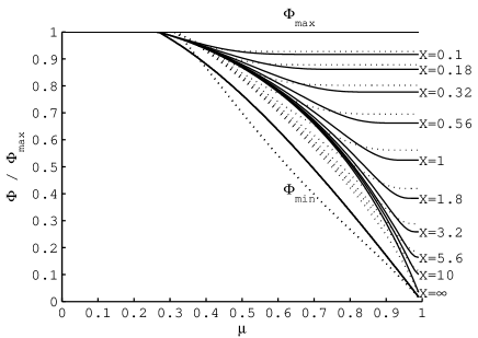
Figure 3: Volume fraction, $\Phi$, vs. friction coefficient, $\mu$, for several values of the compactivity, X, for 2D (solid lines) and for 3D (dotted lines). Volume fractions are normalized according to their maximal values, $\Phi_{max}={\pi}/{\sqrt{12}}\simeq 0.91$ in 2D and $\Phi_{max}={\pi}/{\sqrt{18}}\simeq 0.74$ in 3D. The bounding minimal and maximal volume fractions, $\Phi_{min}$ and $\Phi_{max}$, are also plotted.

III Two Species: segregation

III.1 Mean-Field Model

We would now like to describe a system consisting of two species of grains differing only in frictional properties. The central question we wish to address in such systems is whether the two species mix homogeneously, or segregate into separate domains. For a system of two species denoted A and B, we shall assume we know the compactivity, X, and the friction coefficients, $\mu_{AA}$, $\mu_{AB}$ and $\mu_{BB}$, between two grains of type A, between a grain of type A and a grain of type B, and between two grains of type B, respectively. The considerations presented in the previous section may be used in order to calculate the maximal volumes, $v_{AA}\equiv v_{max}(\mu_{AA})$, $v_{AB}\equiv v_{max}(\mu_{AB})$ and $v_{BB}\equiv v_{max}(\mu_{BB})$, of the Voronoi cells around an A grain surrounded by A grains, an A grain surrounded by B grains (or a B grain surrounded by A grains) and a B grain surrounded by B grains, respectively. We describe a monodisperse system, hence the corresponding minimal volumes are identical for all types of grains and are denoted here by $v_{min}$.

We would now like to write the partition function, Z, for two species and to derive from it the analog of free energy, $Y=-X\log(Z)$, as a function of the concentration $f=\frac{N_{A}}{N}$, where N is the total number of grains and $N_{A}$ is the number of A grains. The constraint on the total number of grains of each species in the system causes us to view $f$ as a local concentration which varies throughout the system. As in the mean-field description of a binary alloy, which is equivalent to the Ising model, a single minimum of $Y(f)$ means the two species tend to get mixed homogeneously at a concentration equal to the global concentration determined from the number of grains of each species. The existence of two minima of $Y(f)$ means that the system tends to separate into domains with two different concentrations. The percentage of the system with each of these two minimizing local concentrations is determined from the global concentration according to the Maxwell construction (see e.g. christian ).

The number of A grains is $N_{A}=fN$ and the number of B grains is $N_{B}=(1-f)N$. In the mean-field approximation the number of A-A contacts is $N_{AA}=f^{2}Nz/2$, the number of A-B contacts is $N_{AB}=f(1-f)Nz$ and the number of B-B contacts is $N_{BB}=(1-f)^{2}Nz/2$, where $z$ is the average number of neighbors per grain, or the average coordination number, which is assumed to be uniform for all types of grains. The contribution of every contact to the total volume is limited according to its type between $2v_{min}/z$ and $2v_{ij}/z$, with i and j denoting A or B for the types of the two grains in contact. The pseudo partition function is:

$$Z =\frac{N!}{(fN)!((1-f)N)!}\left(\int^{v_{AA}}_{v_{min}}e^{-v/X}dv\right)^{f^{2}N}\cdot$$ (9)

$$\cdot \left(\int^{v_{AB}}_{v_{min}}e^{-v/X}dv\right)^{2f(1-f)N}\left(\int^{v_{BB}}_{v_{min}}e^{-v/X}dv\right)^{(1-f)^{2}N}.$$

Not only does $Z$ not depend on $z$ when $z$ is assumed to be uniform for all types of grains, it can easily be seen that when different values of $z$ are assigned to the different types of grains, the same expression is obtained. This is an important result in the analogy between the configurational statistical mechanics of a granular mixture and the Ising model or a binary alloy. In the Ising model spins are arranged on an ordered lattice, all spins have the same number of nearest neighbors, $z$, and the total energy is determined by the states of the spins on all the lattice sites. In a granular system, on the other hand, the disordered spatial configuration determines the volume of the system and every type of grain may have a different number of nearest neighbors, or a different coordination number, which is related to the volume of the Voronoi cell around it, or to the volume it occupies. Due to the different friction coefficients, $z$ varies between the different types of grains, as is indicated in silbert_2002 where the friction dependence of the average number of contacts is investigated. The number of contacts of every type and the contribution of every contact to the total volume depend inversely on $z$, and since only their product enters the total volume of the system, the resulting partition function does not depend on the values of $z$ for the different types of grains . We will soon see where such physical differences between the granular mixture and the Ising model do affect the resulting behaviour of the system.

Using the partition function we now evaluate the free energy:

$$Y(f,X,N) = -X\log(Z)=$$ (10)

$$= XN[f\log(f)+(1-f)\log(1-f)+$$

$$+ 2f(1-f)R(X)-\log(X)-$$

$$- fR_{AA}(X)-(1-f)R_{BB}(X)],$$

where we have used the notations $R_{ij}(X)\equiv\log\left(e^{-v_{min}/X}-e^{-v_{ij}/X}\right)$ and $R(X)\equiv(R_{AA}+R_{BB})/2-R_{AB}$, and the Stirling’s formula has been used to evaluate $\log N!$ for large $N$. Defining $\Delta v_{ij}\equiv v_{ij}-v_{min}$ we see that

$$R(X)=\log\left(\frac{\sqrt{\left(1-e^{-\Delta v_{AA}/X}\right)\left(1-e^{-\Delta v_{BB}/X}\right)}}{\left(1-e^{-\Delta v_{AB}/X}\right)}\right).$$ (11)

We would now like to minimize $Y$ for given overall compositions, $N_{A}$ and $N_{B}$, and for a given compactivity, $X$. Eq. (10) has been derived under the mean-field approximation, therefore it describes the free energy of a region with uniform concentration, $f$. Formally we should now define the local concentration as a spatially dependent coarse grained function, $f(\overrightarrow{r})$, and the free energy as a functional of it, $Y[f(\overrightarrow{r})]=\int Y(f(\overrightarrow{r}))d\overrightarrow{r}$, and to require that $f(\overrightarrow{r})$ minimize $Y$ under the constraint that $\frac{1}{V}\int f(\overrightarrow{r})d\overrightarrow{r}=N_{A}/N$. The spatial integral over all the system of the last three terms in eq. (10), which are linear in $f$, is independent of the function $f(\overrightarrow{r})$. Therefore these terms do not contribute to the minimization of Y, and we need only consider the contribution of the first three terms to Y. We thus obtain an expression similar to the mean-field free energy of an Ising model or of a binary alloy kubo . The “equilibrium” concentration is now determined from:

$$\frac{\partial Y}{\partial f}=XN\left[\log\left(\frac{f}{1-f}\right)+2(1-2f)R(X)\right]=0,$$ (12)

which is equivalent to:

$$2f-1=\tanh\left(R(X)(2f-1)\right).$$ (13)

For $R(X)<1$ the only solution to this equation is $f=0.5$, which corresponds to mixing, while for $R(X)>1$ two different solutions exist and the systems segregates into regions with these two minimizing concentrations. Therefore, the condition for segregation is that $R(X)>1$, where $R(X)$ is given by eq. (11).

Since $R(X\rightarrow 0)=0$, no segregation occurs in the limit of low compactivities. Contrast this to the behavior of the Ising model and binary alloys, where phase separation exists at low temperatures, and specifically in the limit of zero temperature kubo . Here there is a minimal critical compactivity, above which segregation occurs, rather than the maximal critical temperature, bellow which phase separation occurs in the Ising model. The basic difference between the model presented here for granular materials and the Ising model is as follows: In the Ising model the energy of the system is determined only from its topological state. Namely, once the topology of which element is the nearest neighbor of which other elements is specified, the total energy of the system is determined. In the mean-field approximation these topological states are described by the concentration, hence the energy depends only on it. In the granular model presented here a topological state, specifying the types of contacts around every grain, allows for a range of volumes for the Voronoi cells around every grain and therefore for a range of values for the overall volume of the system. As in the Ising model, the topological state is specified by the concentration in the mean-field approximation, however the total volume of the system depends both on the concentration and on the compactivity, X.

The reason for segregation only at high compactivities may be understood to stem from the range of possible volumes in the following way. The Voronoi cells around the grains all have the same minimal volume, $v_{min}$, determined from geometrical considerations. The probability for finding a Voronoi cell in an exited state with a larger volume, $v>v_{min}$, decays as $e^{-v/X}$. Therefore at the limit $X\rightarrow 0$ all Voronoi cells are expected to be found in their ground state, namely to have a volume $v=v_{min}$, independent of the friction of the grains, which only determines the maximal Voronoi cell volume, $v_{max}(\mu)$. Hence, at low compactivities the differences between grains vanish and the two species mix homogeneously. Segregation may occur only at high compactivities, where exited states, which exist due to friction, have a greater “thermodynamic” weight. This occurrence of segregation at high compactivities rather than at low compactivities may explain the frequent appearance of segregation in granular systems, which typically have significant compactivities, since $X=0$ corresponds to a crystalline packing.

Since for $R>0$, $R(X)$ is a monotonic function (as can be seen from eq. (11) which begins at zero, and since the condition for segregation is that $R>1$, there is only a minimal critical compactivity for segregation (and no upper bound above which there is no segregation) so we may determine whether segregation is possible by investigating the high compactivity limit of $R(X)$. This limit may easily be evaluated to be equal to

$$R_{\infty}\equiv R(X\rightarrow\infty)=\log\left(\frac{\sqrt{\Delta v_{AA}\Delta v_{BB}}}{\Delta v_{AB}}\right),$$ (14)

and the condition for the existence of a critical compactivity for segregation for given values of the friction coefficients is that $R_{\infty}>1$.

This condition may be understood in the following way: The free energy, $Y=V-XS$, includes a volume ($V$) term and an entropy ($S$) term. At high compactivities the entropy dominates and minimizing the free energy is equivalent to maximizing the entropy. The entropy includes two factors, a “combinatoric entropy” related to the topological state of the system, namely which grain is in contact with which other grains, and a “geometric” entropy related to the variety of volumes the Voronoi cell around every grain may have within one specific topological state (This is not the case for the Ising model, where the topological state determines the state of the system, and the total entropy includes only the combinatoric entropy, or the entropy of mixing christian ).

The entropy’s dependence on concentration at the limit $X\rightarrow\infty$ is given by

$$S = -N[f\log(f)+(1-f)\log(1-f)+$$ (15)

$$+ 2f(1-f)R_{\infty}].$$

The first two terms are the combinatoric entropy or entropy of mixing, while the last term is the geometric entropy. The geometric entropy plays a similar role to the role of the energy in the Ising model, as can be seen in the expression for the free energy in the Ising model kubo :

$$F = N[kT(f\log(f)+(1-f)\log(1-f))-$$ (16)

$$- 2f(1-f)Jz],$$

where $k$ is the Boltzman constant, $T$ is temperature, $J$ is the interaction energy between neighboring spins and $z$ is the number of nearest neighbors per site. Ising systems exhibit phase separation when $kT<-Jz$, which may now be seen to be completely analogous to the condition $R_{\infty}>1$ for segregation in granular binary mixtures at high compactivities.

III.2 Phase Diagram

We would now like to generate a phase diagram for segregation and to check for which values of $\mu_{AA}$, $\mu_{BB}$ and $\mu_{AB}$ segregation is possible. From mechanical considerations we would expect $\mu_{AB}$ to lie between $\mu_{AA}$ and $\mu_{BB}$. Since $v_{max}(\mu)$ is monotonic, $\Delta v(\mu)$ is monotonic as well, and $\Delta v_{AB}$ is bounded between $\Delta v_{AA}$ and $\Delta v_{BB}$. First we notice that if $\mu_{AB}=max(\mu_{AA},\mu_{BB})$, $R_{\infty}<0$ and no segregation is expected. For given values of $\mu_{AA}$ and $\mu_{BB}$, $R_{\infty}$ varies monotonicaly with $\mu_{AB}$, and a necessary condition for segregation in intermediate values of $\mu_{AB}$ is that there is segregation at $\mu_{AB}=min(\mu_{AA},\mu_{BB})$. In this case

$$R_{\infty}=\log\left(\sqrt{\frac{max(\Delta v_{AA},\Delta v_{BB})}{min(\Delta v_{AA},\Delta v_{BB})}}\right).$$ (17)

Fig. 4 displays the regions in the $\mu_{AA}-\mu_{BB}$ plane where $R_{\infty}>1$, and in which segregation may occur. When $R_{\infty}<1$ the two species are always expected to be mixed. When $R_{\infty}>1$ segregation occurs at the limits of $\mu_{AB}=min(\mu_{AA},\mu_{BB})$ and $X\rightarrow\infty$. Segregation also occurs at larger values of $\mu_{AB}$ and at finite values of $X$. The existence of segregation may be verified for the general case by checking whether the expression for $R(X)$ in eq. (11) is greater than one. Here we only demonstrate our model results for the limits described above. As will be shown in the following subsection, in some cases segregation occurs for every compactivity. The phase diagram shows that mixtures of grains with close friction coefficients will mix and what difference in friction coefficients is needed in order to achieve segregation.

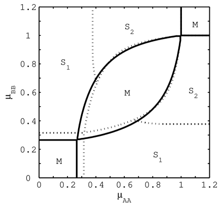
Figure 4: Phase diagram of the $\mu_{AA}-\mu_{BB}$ plane under the assumption that $\mu_{AB}=min(\mu_{AA},\mu_{BB})$ for 2D (solid lines) and 3D (dotted lines). M indicates mixing, $S_{1}$ and $S_{2}$ indicate segregation. M regions are always mixed. In 2D S regions are segregated at high enough compactivity (see text). In 3D $S_{1}$ regions are always segregated, while $S_{2}$ regions are segregated only at high enough compactivity (see section III.3).

Within the framework of the mechanical model used here, frictional forces are relevant only for $0.3\lesssim\mu\leq 1$. If $\mu_{AA}\lesssim 0.3$ or $\mu_{BB}\lesssim 0.3$ it is questionable whether this mechanical model is valid. If both $\mu_{AA}\geq 1$ and $\mu_{BB}\geq 1$ the friction has an identical effect no matter what the values of $\mu_{AA}$ and $\mu_{BB}$ are, therefore the two species mix. If only one of $\mu_{AA}$ or $\mu_{BB}$ is greater than one, the maximal volume per grain of the corresponding species is unbounded, while for the second species it is bounded, leading to $R_{\infty}>1$, and hence to segregation. These regions are designated as well in fig. 4.

III.3 Eliminating the Compactivity

Given the mechanical properties of the grains, namely $\mu_{AA}$, $\mu_{AB}$ and $\mu_{BB}$, we have employed a mean field approximation in order to solve the Edwards statistical mechanics description of a granular mixture and to obtain the concentration (or concentrations in case of segregation) the system will be found at as a function of compactivity. Even though there is evidence that it may be controlled experimentally nowak_1997 ; edwards_grinev_PRE_1998 , the compactivity is still not a measurable quantity, and we would like to reach a description of segregation independent of the notion of compactivity.

For a single species we have seen that the total volume of the system, and correspondingly its volume fraction, depend on compactivity. We shall now derive the compactivity dependence of the volume fraction in a binary mixture, and use it in order to eliminate the compactivity from the description of segregation. This will result in a relation between concentrations and volume fraction, which may be measured experimentally.

The average volume per grain may easily be derived from the partition function (eq. (9)) as:

$$<v> = \frac{<V>}{N}=\frac{1}{N}X^{2}\frac{\partial\ln(Z)}{\partial X}=$$ (18)

$$= X+f^{2}Q_{AA}(X)+2f(1-f)Q_{AB}(X)+$$

$$+ (1-f)^{2}Q_{BB}(X),$$

where

$$Q_{ij}(X) \equiv X^{2}\frac{\partial R_{ij}(X)}{\partial X}=$$ (19)

$$= \frac{v_{min}e^{-v_{min}/X}-v_{ij}e^{-v_{ij}/X}}{e^{-v_{min}/X}-e^{-v_{ij}/X}}.$$

As for a single species, when $X\rightarrow 0$, $Q_{ij}(X)\rightarrow v_{min}$ and $<v>\rightarrow v_{min}$. Moreover, when $X\rightarrow\infty$, $Q_{ij}(X)\approx v_{ij}+v_{min}-X$, hence $<v>\rightarrow v_{min}+f^{2}v_{AA}+2f(1-f)v_{AB}+(1-f)^{2}v_{BB}$.

The concentration $f$ may be expressed as a function of $X$ by using eq. (13). Eliminating $X$ between eq. (13) and (18), we obtain $f$ as a function of the volume fraction, $\Phi$. This is plotted in fig. 5 for typical values of the friction coefficients ($\mu_{AA}=0.35$, $\mu_{BB}=0.75$ and $\mu_{AB}=0.35$). At low compactivities the volume fraction is high and the system is mixed. As the compactivity is raised the volume fraction is reduced and at some critical point segregation commences, and two different concentrations appear. These two values are the concentrations in different domains of the system. As the compactivity is raised above the critical point the two concentrations separate one from each other, enhancing the difference between the different domains. We identify the critical compactivity for segregation, $X_{c}$, above which segregation occurs and the critical volume fraction for segregation, $\Phi_{c}\equiv\Phi(X_{c})$, below which segregation occurs. An important point to note in the case demonstrated in fig. 5 is that in 3D $\Phi_{c}\simeq 0.7$, which is larger than the volume fraction of 3D RCP, $\Phi_{RCP}\simeq 0.64$. Granular materials typically do not reach volume fractions higher than that of RCP, therefore in this case the compactivity is always high enough so that the volume fraction is smaller than $\Phi_{c}$ and segregation always occurs. We now use this argument in order to divide the $\mu_{AA}-\mu_{BB}$ plane into regions where $\Phi_{c}>\Phi_{RCP}$ (denoted $S_{1}$ in fig. 4), which are segregated for all $X$, and regions where $\Phi_{c}<\Phi_{RCP}$ (denoted $S_{2}$ in fig. 4), which are segregated only above some $X_{c}$ (or only under some $\Phi_{c}$). Such considerations may not be used in 2D, where full crystalization is achieved experimentally.

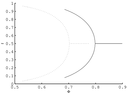
Figure 5: Concentration, $f$, vs. volume fraction, $\Phi$, for $\mu_{AA}=0.35$, $\mu_{BB}=0.75$, $\mu_{AB}=0.35$ for 2D (solid lines) and 3D (dotted lines). For low compactivities (or high volume fractions) a single concentration is possible and the two species mix. For high compactivities (or low volume fractions) two concentrations are possible and segregation occurs.

IV Conclusions:

We have used Edwards’ statistical mechanics hypothesis together with a simple mechanical model to describe the role of friction in 2D and 3D granular materials. For a single species this describes the decrease in volume fraction with increasing friction coefficient and with increasing compactivity. An experimental test of the ideas presented is most easily interpreted for systems differing in friction coefficient but with the same compactivity. It is intriguing to consider whether identical preparation would lead to equal compactivities for systems differing only in friction coefficients.

In addition, the model has been used in order to investigate segregation in binary mixtures of grains differing in frictional properties. Unlike mixtures of grains differing in size, which may be mapped to the Ising model, frictional differences between grains result in larger entropy for the rougher grains; therefore, these systems may not be mapped exactly onto the Ising model, we find that segregation occurs above a critical compactivity and not below it. A phase diagram for segregation vs. friction coefficients of the two species, which may be tested experimentally, has been generated. By eliminating the compactivity, we have also provided a relation between the volume fraction and the nature of mixing or segregation. This relation both provides an option for experimental validation of the model and of the statistical hypothesis and allows to identify mixtures which are expected to segregate at every compactivity.

The geometrical and mechanical models used to describe friction in this paper are more qualitative than quantitative, and more sophisticated models may be suggested. However, the qualitative results obtained here do not depend on their details but only on basic properties which all such models should have: the minimal volume does not depend on friction and the maximal volume and the number of possible states increase with friction. The experimental validation or invalidation of the aforementioned results may shed light on the validity of the statistical mechanics proposal of Edwards.

Appendix A Voronoi Cell Volumes

This appendix describes the calculations leading from the mechanical models in 2D and in 3D to the volume of the corresponding Voronoi cells around the grains, given in eq. (8). In 2D the Voronoi cell around a grain is formed by the tangents to it at the contact points with the surrounding grains. The segment of the Voronoi cell lying between two contacts is the shaded rhombus in fig. 1, which has an area of $r^{2}\tan\theta$, where $r$ is the grain radius and $\theta$ is half the angle between two adjacent contacts. If all angles between adjacent contacts are equal to $2\theta$, the Voronoi cell is comprised of $\pi/\theta$ such segments. Even though this is an integer number only for discrete values of $\theta$, we use this for continuous values of $\theta$. The resulting area of the Voronoi cell is $v_{vor}^{2D}=\frac{\pi r^{2}\tan\theta}{\theta}$.

In 3D we use a triangulation of the contact points on the surface of every grain, and in analogy to the 2D case, we consider the segment of the Voronoi cell bounded between three contacts (see fig. 6).

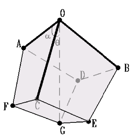
Figure 6: The segment of the 3D Voronoi cell around the grain centered at $O$ and blocked between the three contacts $A$, $B$ and $C$. The tangent planes at the contact points meet the planes formed by the directions to the contact points at $D$, $E$ and $F$ and all meet at $G$.

We assume the three contact points $A$, $B$ and $C$ form an equilateral triangle, therefore $\angle AOG=\angle BOG=\angle COG=\theta$, where $O$ is the center of the grain and $G$ lies on the line directed from $O$ to the center of the triangle $\vartriangle ABC$. The segment of the Voronoi cell is the region bounded between the three directions $OA$, $OB$ and $OC$ (or the planes $AOB$, $BOC$ and $COA$) and the tangent planes $ADGF$, $BEGD$ and $CFGE$ (which due to symmetry meet at the point $G$, which is located along the direction from $O$ to the center of the triangle $\vartriangle ABC$). The segment of the Voronoi cell may be divided into six tetrahedra of equal volume all having the common edge $OG$: $OADG$, $OAFG$, $OBDG$, $OBEG$, $OCEG$ and $OCFG$. Its volume is hence given by

$$v_{seg} = 6v_{OCEG}=6\frac{S_{OCG}H_{E}}{3}=$$ (20)

$$= r^{2}\tan\theta\cdot\frac{\sqrt{3}r\sin\theta}{1+3\cos^{2}\theta},$$

where $S_{OCG}$ is the area of the triangle $\vartriangle OCG$ and $H_{E}$ is the distance of $E$ from the plane of $\vartriangle OCG$. In order to calculate the total volume of the Voronoi cell we calculate the number of segments it is comprised of through the solid angle every such segment occupies. The angle $\angle AOB=\angle BOC=\angle COA=\alpha$ may be calculated from the scalar product of any two of the vectors $OA$, $OB$ and $OC$ and is given by $\cos\alpha=(3\cos 2\theta+1)/4$. The solid angle formed by these three vectors is $\Omega=4\tan^{-1}\left(\sqrt{\tan(3\alpha/4)\tan^{3}(\alpha/4)}\right)$. Therefore the Voronoi cell volume is

$$v_{vor}^{3D} = v_{seg}\frac{4\pi}{\Omega}=$$ (21)

$$= \frac{\pi r^{3}\sqrt{3}\sin\theta\tan\theta}{(1+3\cos^{2}\theta)\tan^{-1}\left(\sqrt{\tan\frac{3\alpha}{4}\tan^{3}\frac{\alpha}{4}}\right)}.$$

References

- (1) S.F. Edwards and R.B.S. Oakeshott, Physica A 157, 1080 (1989).
- (2) B.H. Kaye, Powder Mixing (Chapman & Hall, London, 1997).
- (3) G.H. Ristow, Pattern Formation in Granular Materials, Vol. 164 of Springer Tracts in Modern Physics (Springer, Berlin, 2000).
- (4) F. Cantelaube and D. Bideau, Europhys. Lett. 30, 133 (1995).
- (5) L.R. Lawrence and J.K. Beddow, Powder Technol. 2, 253 (1968).
- (6) O. Zik, D. Levine, S.G. Lipson, S. Shtrikman and J. Stavans, Phys. Rev. Lett. 73, 644 (1994).
- (7) T. Shinbrot and F. Muzzio, Phys. Rev. Lett. 81, 4365 (1998).
- (8) W. Cooke, S. Warr, J.M. Huntley and R.C. Ball, Phys. Rev. E 53, 2812 (1996).
- (9) J.B. Knight, H.M. Jaeger and S.R. Nagel, Phys. Rev. Lett. 70, 3728 (1993).
- (10) H.A. Makse, S. Havlin, P.R. King and H.E. Stanley, Nature 386, 379 (1997).
- (11) J.C. Williams, Powder Technol. 15, 245 (1976).
- (12) J.M. Ottino and D.V. Khakhar, Annu. Rev. Fluid Mech. 32, 55 (2000).
- (13) E. Clment, J. Rajchenbach and J. Duran, Europhys. Lett. 30, 7 (1995).
- (14) D. Levine, Chaos 9, 573 (1999).
- (15) P.Y. Lai, L.C. Jia, and C.K. Chan, Phys. Rev. Lett. 79, 4994 (1997).
- (16) T. Boutreux and P.G. de Gennes, J. Phys. I France 6, 1295 (1996).
- (17) A. Rosato, K.J. Strandburg, F. Prinz and R.H. Swendsen, Phys. Rev. Lett. 58, 1038 (1987).
- (18) A. Mehta and G.C. Barker, Phys. Rev. Lett. 67, 394 (1991).
- (19) T. Boutreux and P.G. de Gennes, Physica A 244, 59 (1997).
- (20) E. Ben-Naim, J.B. Knight, E.R. Nowak, H.M. Jaeger and S.R. Nagel, Physica D 123, 380 (1998).
- (21) E.R. Nowak, J.B. Knight, E. Ben-Naim, H.M. Jaeger and S.R. Nagel, Phys. Rev. E 57, 1971 (1998).
- (22) S.A. Langer and A.J. Liu, Europhys. Lett. 49, 68 (2000).
- (23) I.K. Ono, C.S. O’Hern, D.J. Durian, S.A. Langer, A.J. Liu and S.R. Nagel, Phys. Rev. Lett. 89, 095703 (2002).
- (24) A. Barrat, J. Kurchan, V. Loreto and M. Sellitto, Phys. Rev. Lett. 85, 5034 (2000).
- (25) H.A. Makse and J. Kurchan, Nature 415, 614 (2002).
- (26) E.R. Nowak, J.B. Knight, M.L. Povinelli, H.M. Jaeger and S.R. Nagel, Powder Technol. 94, 79 (1997).
- (27) S.F. Edwards and D.V. Grinev, Phys. Rev. E 58, 4758 (1998).
- (28) A. Mehta and S.F. Edwards, Physica A 157, 1091 (1989).
- (29) R. Blumenfeld and S.F. Edwards, Phys. Rev. Lett. 90, 114303 (2003).
- (30) P. Richard, L. Oger, J.P. Troadec and A. Gervois, Eur. Phys. J. E 6, 295 (2001).
- (31) L.E. Silbert, D. Ertas, G.S. Grest, T.C. Halsey and D. Levine, Phys. Rev. E 65, 031304 (2002).
- (32) J.W. Christian, The Theory of Transformations in Metals and Alloys, Vol. 15 of International Series on Materials Science and Technology, 2nd ed. (Pergamon Press, Oxford, 1981).
- (33) R. Kubo, Statistical Mechanics - An Advanced Course with Problems and Solutions, 8th ed. (North-Holland, Amsterdam, 1990).