Dimensional Crossover of Localisation and Delocalisation in a Quantum Hall Bar

Abstract

The 2– to 1–dimensional crossover of the localisation length of electrons confined to a disordered quantum wire of finite width $L_{y}$ is studied in a model of electrons moving in the potential of uncorrelated impurities. An analytical formula for the localisation length is derived, describing the dimensional crossover as function of width $L_{y}$, conductance $g$ and perpendicular magnetic field $B$ . On the basis of these results, the scaling analysis of the quantum Hall effect in high Landau levels, and the delocalisation transition in a quantum Hall wire are reconsidered.

]

I INTRODUCTION

The Hall conductance of a 2–dimensional electron system in a strong magnetic field [1] is precisely quantised due to the trapping of electrons to localized states in the bulk of the system. Thereby, a change of electron density does not result in a change of the Hall conductance[2, 3, 4]. In the tail of the Landau bands the localisation length $\xi$ is small, on the order of the cyclotron length $l_{cyc}=\sqrt{2n+1}l_{B}$, where the magnetic length $l_{B}$ is defined by $l_{B}^{2}=\hbar/(qB)$. The localisation length increases towards the middle of the Landau bands, located at energies $E_{n}=\hbar\omega_{c}(n+1/2)$, where $\omega_{c}=qB/m$ is the cyclotron frequency, q being the electron charge, and $n=0,1,2,...$. In an infinite system the localisation length of an Eigen state with energy $E$ is expected to diverge as $\xi\sim(E-E_{n})^{-\nu}$. The exponent $\nu$ is found for the lowest two Landau bands, $n=0,1$ to be $\nu\approx 2.3$ for spin split Landau levels, as supported by analytical[5, 6], numerical [7, 8] and experimental studies [9], reminiscent of a second order transition from an insulator to a metal. Thus, for a finite system, there should exist in the middle of a disorder broadened Landau–band, $E_{n}$, n being the Landau index, a band of states, which extend through the whole system of size $L$, with band width $\Delta E=(l_{cyc}/L)^{1/\nu}\Gamma$, where $\Gamma=\hbar\sqrt{2/\pi}\sqrt{\omega_{c}/\tau}$.

On the other hand, the localisation length in two–dimensinal systems with broken time reversal symmetry is from the one parameter scaling theory expected to depend exponentially on the conductance $g$ as [10, 11, 12, 13]

$$\xi\sim\exp(\pi^{2}g^{2}).$$ (1)

$g$ is the conductance parameter per spin channel. $g$ exhibits the Shubnikov-de-Haas oscillations as function of the magnetic field, for $\omega_{c}>1/\tau$, where $1/\tau$ is the elastic scattering rate. The maxima occur, when the Fermi energy is in the middle of the Landau band. Thus, the localisation length is expected to increase strongly from the tails to the middle of the Landau bands, irrespective of the existence of the quantum critical point. For uncorrelated impurities, within self consistent Born approximation[14], one finds that the maxima in the longitudinal conductance are given by $g(E=E_{n})=\frac{1}{\pi}(2n+1)=g_{n}$. Thus, one gets localisation lengths $\xi_{2D}(E_{n})=l_{\rm cyc}\exp(\pi^{2}g_{n}^{2})$ in the middle of higher Landau levels, $n>1$, which are macroscopically large[8, 15]. However, when the width of the wire $L_{y}$ is smaller than the length scale $\xi$, the localisation is expected to become quasi–1–dimensional. That is, the electrons in the middle of a Landau band can diffuse freely between the edges of the wire, but are localised along the wire. The quasi-1-dimensional localisation length is known to depend only linearly on the conductance, and is, in a magnetic field, with broken time reversal symmetry, given by[16, 17, 18, 19]

$$\xi=2g(B)L_{y}.$$ (2)

Thus, for $L_{y}\ll\xi_{2D}(E_{n})$ there is a crossover from 2– to 1–dimensional localisation as the Fermi energy is moved from the tails into the middle of a Landau band. It is known from numerical [7] and analytical studies [6], that in a finite quantum Hall bar, the criticality in the middle of the Landau band results in a finite localisation length $\xi_{crit}\approx 1.2L_{y}$, exceeding the wire width $L_{y}$. Comparing this value with the quasi–1–dimensional localisation length for uncorrelated impurities in the middle of the Landau band, obtained from Eq. (2), $\xi_{n1D}=\frac{2}{\pi}(2n+1)L_{y}$, we see that this length scale exceeds the critical localisation length $\xi_{crit}$ in all but the lowest Landau level, $n=0$.

It is the aim of this article to derive analytically the dimensional crossover of the localisation length $\xi$ in a wire as function of a perpendicular magnetic field. This might also help to identify the irrelavent scaling parameters observed in numerical studies of the integer quantum Hall transition[7, 8]. We also find that in quantum Hall bars of finite width $L_{y}$, there exists at low temperatures a new phase, when the phase coherence length $L_{\varphi}$ exceeds the quasi–1–dimensional localisation length, in the middle of the Landau band, $L_{\varphi}>\xi_{n}$[20]. This phase may accordingly be called the mesoscopic quantum Hall phase, exhibiting plateaus in the Hall conductance, when the bulk localisation length is smaller than the wire width, and the Hall conductance is carried by edge states, separated by regions in energy where all states are localised along the wire, and the conductance is zero. A similar result has also been noted recently in a renormalization group study of a quantum Hall bar in Ref. [6].

In the next section the crossover between 1–dimensional and 2–dimensional localisation is studied. In the third section the localisation length is derived as function of magnetic field. In the fifth section, the scaling theory of the integer quantum Hall effect is considered. It is shown that the irrelevant scaling parameter and the scaling function is in qualitative agreement with the one obtained from the noncritical theory. In the last section, a summary is given, and implications of these results for the theory of the integer quantum Hall effect are pointed out. The derivations are given in appendices A ( orthogonal localisation length as function of wire width $L_{y}$), B ( unitary localisation as function of wire width $L_{y}$), and C (orthogonal to unitary crossover of 2D localisation length). In Appendix D a generalized derivation of the field theory including an edge state potential and the topological term in the presence of a magnetic field is given.

II Dimensional crossover of localisation

In the follwing, we study the localisation length $\xi$ of electrons confined to a disordered wire of finite width $L_{y}$.

Orthogonal Regime. First, let us consider the problem without magnetic field, $B=0$, the orthogonal regime.

An estimate of the localisation length $\xi$ can be obtained by performing a perturbative renormalization of the dimensionless conductance $g$, which appears as the coupling constant of the action in the nonperturbative theory of disordered electrons. The bare conductance $g$ is obtained in self consistent Born approximation[14]. The vanishing of the renormalised conductance $\tilde{g}\rightarrow 0$ as one increases the wavelength of renormalisation, signals the localisation, and can be used to obtain an estimate of the localisation length $\xi$, as done in appendix A.

The first order in $1/g$ of the perturbative renormalization corresponds to the weak localisation correction to the conductivity. Thus, one can estimate the localisation length $\xi$ at zero magnetic field $B=0$ as done in appendix A. There, the renormalisation is performed for arbitrary finite widths $L_{y}$ of the wire. One thus gets the following equation for the localisation length $\xi$,

$$\xi=gL_{y}-\frac{L_{y}}{\pi}\ln\left[2\frac{k_{0}L_{y}/(2\pi)}{1+\sqrt{1+(L_{y}/(2\pi\xi))^{2}}}\right].$$ (3)

where $k_{0}=2\pi/l=\pi k_{F}/g$, and we assumed that the wire width is diffusive, $L_{y}>l$.

In the quasi-1-D limit, $\xi\gg L_{y}$, we find a logarithmic correction, to the expected quasi-1- D result, $\xi=gL_{y}$:

$$\xi=gL_{y}-\frac{L_{y}}{\pi}\ln(k_{F}L_{y}/g).$$ (4)

In the opposite limit, $\xi\ll L_{y}$, the nonlinear equation for the localisation length simplifies to,

$$\xi=l\exp(\pi g)\exp(-\pi\frac{\xi}{L_{y}}).$$ (5)

FIG. 1.: The width dependence of the localisation length $\xi$ at fixed conductance $g=2$ without magnetic field, $B=0$, is shown as the full line. For comparison, the quasi–1–dimensional limit $L_{y}g$ is drawn as the dash–dotted line. The crossover occurs at $\xi=L_{yc}=\exp(-\pi)(2g/k_{\mbox{F}})\exp(\pi g)$.

The solution of this equation can be written in closed form in terms of the Lambert–W–function $W_{0}(z)$[21]:

$$\xi=\frac{L_{y}}{\pi}W_{0}(\frac{2\pi}{L_{y}}\frac{g}{k_{\mbox{F}}}\exp(\pi g)),$$ (6)

where we substituted $l=2g/k_{\mbox{F}}$. The Lambert–W–function $W_{0}(x)$ is defined as the solution of the nonlinear equation[21]

$$z=a\exp(-bz),$$ (7)

given by

$$z=\frac{1}{b}W_{0}(ab).$$ (8)

Thus, the localisation length is found to increase linearly with the width like

$$\xi\mid_{\xi\gg L_{y}}=gL_{y},$$ (9)

when the localisation length exceeds the width $L_{y}$, $\xi\gg L_{y}$. It logarithmically deviates from this behavior when the width $L_{y}$ is on the order of $L_{yc}=\exp(-\pi)l\exp(\pi g)$. For larger widths, it slowly saturates towards the width independent 2D–localisation length,

$$\xi\mid_{\xi\ll L_{y}}=\frac{2g}{k_{\mbox{F}}}\exp(\pi g),$$ (10)

as seen in Fig. 1.

For internediate widths there is a wide regime where the localisation lengths deviate strongly from both 1–D, Eq. (9), and 2–D, Eq. (10), which would yield $\xi_{2D}(g=2)=2142$ on the scale $1/k_{F}$, used in Fig. 1.

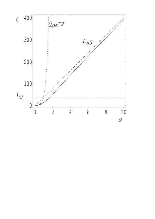
FIG. 2.: The localisation length $\xi$ (fulll line) in units of $k_{\mbox{F}}^{-1}$ as function of the conductance $g$ at fixed width $L_{y}=40$, and without magnetic field, $B=0$. It is plotted using Eq. (6) for $\xi<L_{y}$, and Eq. (4) for $\xi>L_{y}$. For comparison, we show the quasi–2–dimensional $\xi_{2D}=(2g/k_{\mbox{F}})\exp(\pi g)$ (dashed line) and the quasi–1–dimensional $L_{y}g$ (dash–dotted line) limiting functions.

As one fixes the width $L_{y}$, and increases the dimensionless conductance $g$, a crossover from 2D– to 1D–localisation is observed, as shown in Fig. 2. There, Eq. (6) is plotted as function of $g$, for $\xi<L_{y}$. For $\xi>L_{y}$, the localisation length is plotted using, Eq. (4). In the intermediate regime, the solution of the general equation Eq. (3) deviates only little from these asymptotic solutions. Note that the validity of the derivation is limited to $g>1$, while the deviations from 2D localisation behavior occur for the chosen width $L_{y}$ already close to $g=1$. The derivation given above has been done for wires of diffusive width, $l<L_{y}$, or $g<L_{y}k_{\mbox{F}}/2$, corresponding to $g<20$ in Fig. 2.

Unitary Regime. At moderately strong magnetic field, the time reversal symmetry is broken, and the so called unitary regime is reached, when the localisation length exceeds the magnetic diffusion length[22], $\xi>L_{B}$, (where $L_{B}=l_{B}$, when $l_{B}<L_{y}$ and $L_{B}=(3)^{1/2}l_{B}^{2}/L_{y}$, when $l_{B}>L_{y}>l$). Then, the first order, weak localisation correction vanishes and one needs to do the perturbative renormalisation to second order in $1/g$. Thus, we have to calculate all diagrams contributing to this order, the so called Hikami boxes[12], to study the dimensional crossover in a magnetic field. An efficient way to do this, is to start from the supersymmetric nonlinear sigma model and do an expansion around its classical point, as done in Ref. [16] for the pure orthogonal and unitary regimes in 2 dimensions.

Performing this renormalisation for wires of finite width $L_{y}$ in the unitary regime, we obtain in appendix B, that the localisation length $\xi$ satisfies in the unitary regime the equation,

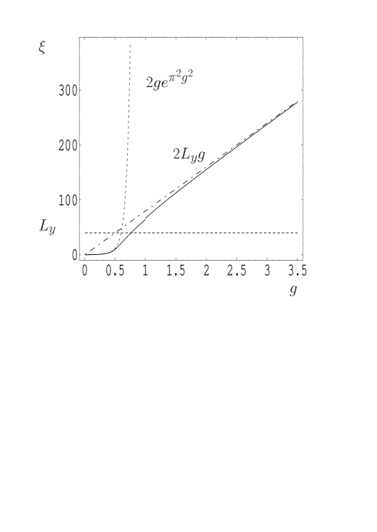
FIG. 3.: The localisation length $\xi$ as function of conductance $g$, for large enough magnetic fields such that $\xi>L_{B}$, at fixed width $L_{y}$. For comparison, the quasi–2–dimensional behavior $\xi_{2D}=2(g/k_{\mbox{F}})\exp(\pi^{2}g^{2})$ ( dotted line) and the quasi–1–dimensional limit $L_{y}g$ (dash–dotted line). The width $L_{y}$ is indicated by the dashed line.

$$\xi^{2}=L_{y}^{2}\left(\Sigma^{2}(4g^{2}-1)+\frac{2}{\pi^{2}}\ln\left[\frac{1+(\xi/(2\pi L_{y}))^{2}}{1+(\xi k_{0})^{2}}\right]\right).$$ (11)

Here, the length scale $2\pi/k_{0}$ is the short distance cutoff of the nonperturbative theory, being $l=2g(B=0)/k_{F}$ at moderate magnetic fields, when $\omega_{c}\tau<1$, and crossing over to the cyclotron length $l_{\rm cyc}$ at strong magnetic fields when $\omega_{c}\tau>1$.

Here, $\Sigma=1$, unless the spin degeneracy is broken, and the energy levels are mixed by spin flip as by scattering from magnetic impurities, then $\Sigma=2$. Note that the above results confirm the result for the localisation length in the quasi–1–D limit [17, 18],

$$\xi\mid_{\xi\gg L_{y}}=\Sigma\beta gL_{y},$$ (12)

where $\beta=1,2$ with, without time reversal symmetry. We will set $\Sigma=1$ in the following. We can solve Eq. (11) in two limiting cases. When $L_{y}\ll\xi$, the quasi–1–dimensional localisation length is obtained with a logarithmic correction,

$$\xi\mid_{\xi\gg L_{y}}=2L_{y}g\left[1-\frac{1}{\pi^{2}g^{2}}\ln\sqrt{1+\left(L_{y}k_{0}/(2\pi)\right)^{2}}\right]^{1/2}.$$ (13)

In the limit of 2–dimensional localisation, $\xi\ll L_{y}$, the localisation length is found to satisfy the equation

$$\xi\mid_{\xi\ll L_{y}}=\frac{2\pi}{k_{0}}\exp\left[\frac{\pi^{2}}{4}(4g^{2}-\frac{\xi^{2}}{L_{y}^{2}})\right].$$ (14)

Its solution can be written in terms of the Lambert–W–function[21] as

$$\xi=\frac{\sqrt{2}L_{y}}{\pi}W_{0}^{1/2}\left[\frac{2\pi^{4}}{k_{0}^{2}L_{y}^{2}}\exp(2\pi^{2}g^{2})\right].$$ (15)

Fixing the width $L_{y}$ the dimensional crossover is seen in Fig. 3, where the localisation length is plotted as function of the dimensionless conductance g, using Eq. (13) for $\xi>L_{y}$, and Eq. (15) for $\xi<L_{y}$.

III The magnetic field dependence of the localisation length

Weak magnetic field

In disordered quantum wires without strong spin–orbit scattering or magnetic impurities, the electron localisation length is enhanced by a weak magnetic field. If the localisation is quasi–1–dimensional, $\xi>L_{y}$, then the magnetic field results in a doubling, Eq. (12), $\xi=\beta gL_{y}$, where $\beta=1,2$, corresponding to no magnetic field, and finite magnetic field, respectively[17, 18]. Recently, such a doubling of the localisation length was observed experimentally [23]. That doubling is governed by the magnetic diffusion length $L_{B}=(D\tau_{B})^{1/2}$, where $\tau_{B}$ is the magnetic phase shifting time, which is a function of magnetic length $l_{B}$, mean free path $l$ and width of the wire $L_{y}$ [22]. Thus, the localisation length crosses over to $\xi=2gL_{y}$, when the magnetic diffusion length becomes smaller than the localisation length, $L_{B}<\xi$.

This crossover has recently been derived analytically[19, 22]. The quasi–1–D localisation length, valid for $\xi>L_{y}$, is obtained to be given by:

$$\xi(B)=2f(L_{B}/\xi(0))gL_{y}.$$ (16)

Here,

$$f(x)=2/(2+\sqrt{49+64X^{2}}-\sqrt{25+64X^{2}}).$$ (17)

For a wire of diffusive width $W>l$, one finds, $X=\xi(0)/L_{B}=\pi^{2}3^{-1/2}N^{2}b$, where $N_{y}=k_{\mbox{F}}L_{y}/\pi$ is the number of transverse channels, and $b=\omega_{c}\tau=eB\tau/m$ the dimensionless magnetic field parameter. The factor $64$ was not noticed in a previous publication [22], and is a consequence of the particular properties of the autocorrelation function of spectral determinants, and its relation to the actual localisation length which was used to derive Eqs. (16,17) [22]. When the localisation is 2–dimensional, the localisation length $\xi$ becomes exponentially enhanced. The crossover between the orthogonal, Eq. (10), and unitary, Eq. (1), localisation length is governed by the parameter $X=\xi/L_{B}$. Extending the perturbative renormalisation, by calculating the Hikami boxes as a function of magnetic field as outlined in appendix B ( This problem, the magnetic field induced crossover of the weak localisation corrections to the conductivity, has been considered to 2 nd order in $1/g$ also in Ref. [26], using the complex matrix model), one obtains the following equation for the 2D–localisation length,

$$\xi=l\exp(\pi g)(1+X^{2})^{1/2-1/(2\pi g)}\mid_{X=\xi/L_{B}}.$$ (18)

Thus, when the time reversal symmetry is broken, $\xi>L_{B}$, the localisation is given by Eq. (13) for $\xi>L_{y}$, and Eq. (15) for $\xi<L_{y}$, respectively. The effective short distance cutoff of the renormalisation is a function of the magnetic field itself. We get $2\pi/k_{0}=l$ at small magnetic fields, $b<1$, and $2\pi/k_{0}=l_{cyc}$ at large fields from the renormalisation of the diffusive nonlinear sigma model. But, we should note that an analysis of the nonlinear sigma model on ballistic scales is needed to get more reliable information on $1/k_{0}$.

Strong magnetic field

In the following, we consider a quantum wire of disordered electrons in a strong magnetic field, which is expected to exhibit the quantum Hall effect, when its width $L_{y}$ and the mean free path $l$ do exceed the cyclotron length $l_{c}$. We consider quantum Hall wires of diffusive width, where the mean free path is smaller than the wire width, $l<L_{y}$. In the opposite limit, $l>L_{y}$, the ballistic motion between the edges of the wire leads to anomalous magnetoresistance phenomena due to classical commensurability effects of cyclotron orbits with the confinement potential of the wire [24, 25]. This will not be pursued here, since these effects are not related to disorder induced quantum localisation, which is the focus of this article. $\sigma_{xx}(B)$ is the conductivity in self consistent Born approximation. For weak magnetic field, $b<1$, it is identical to the Drude result $\sigma_{xx}=ne^{2}\tau/(1+b^{2})$. With the electron density $n_{e}=Em/(2\pi\hbar^{2})$ this can be rewritten as $g(b)=\sigma_{xx}/\sigma_{0}=g/(1+b^{2})$, where $g=E\tau/\hbar$ per spin channel. Fixing the electron density $n_{e}$, the Fermi energy depends on magnetic field $E_{F}(B)$ for $b>1$. In the following, we will fix the Fermi energy $E_{F}$, instead.

The conductivity in SCBA for $b>1$, when the cyclotron length $l_{c}$ becomes smaller than the mean free path $l$, or $\omega_{c}>1/\tau$, and disregarding the overlap between Landau bands, is given by

$$g(B)=\frac{1}{\pi}(2n+1)(1-(E_{F}-E_{n})^{2}/\Gamma^{2}),$$ (19)

for $\mid E-E_{n}\mid<\Gamma$, where $\Gamma^{2}=(2/\pi)\hbar^{2}\omega_{c}/\tau$, for $\Gamma<\hbar\omega_{c}$.

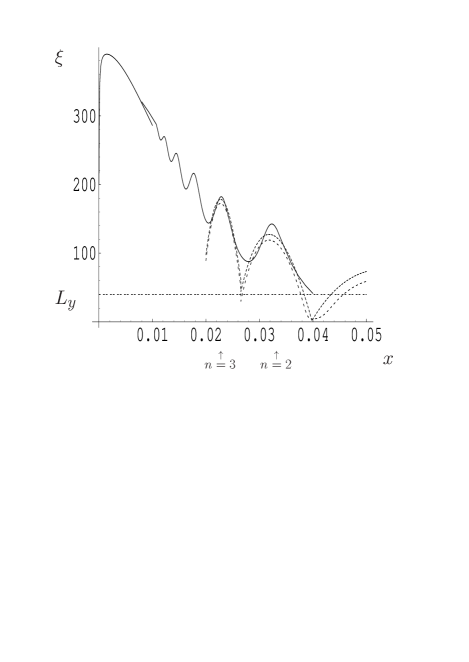
FIG. 4.: The localisation length as function of magnetic flux through a unit cell of area $a^{2}=1/k_{F}^{2}$, $x=\frac{a^{2}}{2\pi l_{B}^{2}}$, with conductance parameter $g(B=0)=10$. For weak magnetic field, Eq. (16) is used. For strong magnetic fields the localisation length is plotted by inserting $g(B)$ in the 2 nd order Born approximation in the formula for the quasi-1-dimensional localisation length, Eq. (2), including a summation over all Landau levels (full line). The short dashed line is obtained by using the self consistent Born approximation (SCBA) for g(B) for one Landau band, Eq. (20), and inserting it into the formula for the quasi-1-dimensional localisation length, Eq. (2). The long dashed curve denotes the correpsonding result using the SCBA conductance and inserting it in the crossover formula Eq. (15). The width of the wire $L_{y}=40a$ is indicated as the horizontal dashed line.

One obtains thus the localisation length for $b>1$ and $\mid\epsilon/b-n-1/2\mid<1$, by substituting the expression for the dimensionless conductance Eq. (19), into Eq. (13) for $\xi>L_{y}$, and Eq. (15) for $\xi<L_{y}$, respectively. Thus, the localisation length is found to oscillate between maximal values in the middle of the Landau bands, and minimal values on the order of the cyclotron length $l_{\rm cyc}$ in the tail of the Landau bands, as seen in Fig. 4.

The localisation is quasi–1–dimensional as long as $\xi(W)>L_{y}$. We see that for $n>1$ this is, for uncorrelated disorder potential, practically always the case in the middle of the Landau bands, with a logarithmic correction as given by Eq. (10), yielding

$$\xi_{n}=\frac{2}{\pi}(2n+1)L_{y}\left[1-\frac{1}{(2n+1)^{2}}\ln\sqrt{1+\left(\frac{L_{y}}{l_{\rm cyc}}\right)^{2}}\right]^{1/2}.$$ (20)

Only in the lowest Landau band, Eq. (2) gives a value for the localisation in the middle of the Landau bands $\xi(B)\approx(2/\pi)L_{y}$, for $n=0$, which is smaller than the width $L_{y}$. Thus, in the lowest Landau band the NLSM is 2-dimensional and the topological term becomes fully effective already for small widths $L_{y}$, see Appendix D. There, the gap in the action of the nonlinear sigma model is diminished due to the presence of the topological term $\sigma_{\rm xy}\neq 0$. Then, there are excitations with nonvanishing topological charge $q$, like Skyrmions which give a phase $\exp(i2\pi q\sigma_{\rm xy})$ to the functional integral. For $\sigma_{\rm xy}=(2n+1)/2$, the skyrmions with $q=\pm 1$ give the opposite sign to the functional integral, $\exp(i\pi)=-1$ than configurations without topological charge, $q=0$, like vortices[27]. Thus, the presence of the topological term leads to quantum criticality, and a diverging localisation length, there. For a wire of finite width, the localisation length then saturates to its critical values which was found numerically to be $\xi_{c}\approx 1.2L_{y}$[7], while analytical estimates exceed this value [6].

We note that we have assumed in the derivation of Eqs. (18,20), that the conductivity is homogenous. In a strong magnetic field, the formation of edge states can result in strongly inhomogenous and anisotropic conductivity, thereby preventing the mixing of edge states with the bulk states[28, 29]. The consequences of these effects will be discussed in more detail, in the next chapter and in a forthcoming article, including a numerical analysis[20].

In a real sample there exists a slowly varying potential disorder which is known to stabilize the edge states against mixing with bulk states and back scattering [30, 31]. But in the middle of the Landau bands there is always scattering from the edge states into the bulk [28], so that quasi–1–dimensional localisation should occur for large aspect ratios of the quantum hall bar, $L\gg L_{y}$.

IV Scaling Function

In the above analysis of a disordered wire in a magnetic field we disregarded the effect of the topological term, which appears in a derivation of the nonlinear sigma model[27, 32, 33], see Eq. (D16). It is known that in the two-dimensional limit this topological term is needed in order that the field theory becomes critical in the middle of Landau bands, and the quantum–Hall–transition from localised states in the Landau band tails to a critical state in the middle of the Landau bands can be described[27, 32, 33, 34, 35, 36]. Can one still learn something about the quantum Hall transition from knowing the noncritical localisation length as function of magnetic field, $\xi(B)$, as derived above, as function of the wire width $L_{y}$?

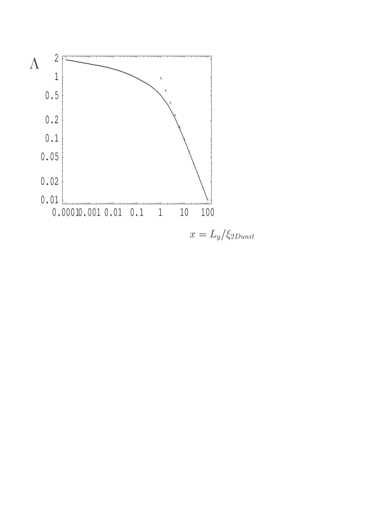
FIG. 5.: The noncritical scaling function obtained analytically (full line), Eqs. (22,23), for the Landau band, $n=3$, with $g_{n}=7/\pi$. The dashed line, $1/x$, is approached in the 2 D limit, when the localisation length becomes equal to $\xi_{2Dunit}$.

Both in numerical calculations [7] and experiments one needs to perform a finite size scaling analysis in order to extract the critical divergence of the localisation length, $\xi\sim(E-E_{n})^{-\nu}$, when approaching the middle of a Landau band, $E_{n}$. The procedure is to find numerically the scaling function $\Lambda=\xi/L_{y}=\Lambda(L_{y}/\tilde{\xi}(E))$, rescaling with the critical localisation length, which diverges according to $\tilde{\xi}(E)\sim(E-E_{n})^{-\nu}$, and does not depend on width $L_{y}$. Then, one can determine $\nu$ by optimizing the accuracy of scaling. The scaling function is not known a priori. It is clear that $\Lambda(x)\rightarrow 1/x$ for $x\gg 1$, since in the tails of the Landau band $\xi\ll L_{y}$, and $\xi$ becomes independent of $L_{y}$, approaching $\tilde{\xi}$.

For the higher Landau bands, $n>0$, the single parameter scaling is not accurate, and it is important to include also irrelevant scaling parameters[37], apart from the relevant parameter, $L_{y}/\tilde{\xi}(E)$ [7, 38]. So far the irrelevant scaling parameters have been included in the numerical scaling analysis on a phenomenological ground, without a precise knowledge of their physical origin. It has been observed, however, that the irrelavent scaling length increases by orders of magnitude in higher Landau bands, for uncorrelated disorder[7].

Therefore, it seems worthwhile to first analyse, if the noncritical width dependence of $\xi(B)$, derived above, Eq. (3), can yield analytical knowledge on the scaling function $\Lambda(x)$ and moreover account for the observed irrelevant scaling parameter in higher Landau bands. Only then will we try to implement the topological term in the derivation of the scaling function at the end of this section.

According to Eq. (23), the ratio $\Lambda$ scales with the large length scale $\xi_{2Dunit}$, which is a huge length scale in the middle of higher Landau bands, where $g\gg 1$. Therefore, it is natural to expect that $\xi_{unit}$ can be identified with the irrelevant length scale $l_{irr}$, and to compare the scaling function, Eqs. (22,23), with the one obtained numerically, Eq. (24).

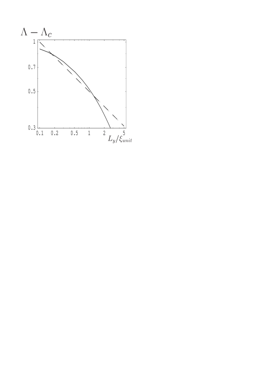
FIG. 6.: The irrelevant scaling function obtained analytically for the Landau band $n=1$, $g=3/\pi$ (full line) as compared with the function Eq. (24) (dashed line), for $\gamma=.3$ and $c=.5$, double logarithmic scale .

In Fig. 5, we plot the scaling function, as obtained above, Eqs. (13,15), as function of $x=L_{y}/\xi_{2Dunit}$, where $\xi_{2Dunit}$ is the 2D limiting value of the unitary localisation length,

$$\xi_{2Dunit}=\frac{2\pi}{k_{0}}\exp(\pi^{2}g^{2}).$$ (21)

Thus, Eqs. (13,15) become

$$\Lambda=\frac{2}{\pi}\sqrt{-\ln\sqrt{x^{2}+(2\pi/k_{0}\xi_{2Dunit})^{2}}},$$ (22)

for $x=L_{y}/\xi_{2Dunit}<\exp(-\pi^{2}/4)\approx.085$, while

$$\Lambda=\frac{\sqrt{2}}{\pi}\sqrt{W_{0}\left(\frac{\pi^{2}}{2}\frac{1}{x^{2}}\right)},$$ (23)

for $x=L_{y}/\xi_{2Dunit}>\exp(-\pi^{2}/4)$. This noncritical scaling function is plotted in Fig. 5, where $g=7/\pi$ has been chosen, corresponding to the unrenormalised conductance in the Landau band, $n=3$. We note that the derivation is only valid for $g\gg 1$, so that we are able to compare this function only with the scaling function in higher Landau bands, where $g_{n}\gg 1$. It is expected that this noncritical scaling function is accurate as long as $x=L_{y}/\xi_{2Dunit}<1$.

Close to the critical point, $x=L_{y}/\xi_{2Dunit}\gg 1$, the scaling function is from the numerical analysis obtained to be in the middle of the Landau band

$$\Lambda-\Lambda_{c}=\frac{\xi}{L_{y}}=c(\frac{L_{y}}{l_{irr}})^{-\gamma},$$ (24)

where $\Lambda_{c}=1.2$, and the irrelevant critical scaling exponent is numerically found to be $\gamma=.38\pm.04$, and $c$ is a constant.

In Fig. 6, we plot $\Lambda-\Lambda_{c}$, Eq. (24) using $\gamma=.3$ and $c=.5$, and compare it with $\Lambda$ as obtained from the result of the noncritical analysis, Eq. (23). Note that this function converges to zero as $L_{y}\rightarrow\infty$, corresponding to $\Lambda_{\rm crit}=0$, since it was obtained from the noncritical field theory, disregarding the topological term. Thus, as expected, the form of the noncritical irrelevant scaling function defers from the results of the numerical analysis as seen in Fig. (6), but is in some quantitative agrrement. Inspite of this, it is expected that the scaling function itself is changed by the presence of the critical point in the middle of the Landau band, and the similarity to the noncritical scaling function derived above, is only of qualitative nature. Since in higher Landau levels one is in the study of wires of finite width $L_{y}$ for uncorrelated disorder always far away from the critical point, as shown above, we conclude that this noncritical scaling function is important in order to enable one to analyse the quantum Hall transition in higher Landau bands, $n>1$. We can estimate the region of criticality by the condition that $\tilde{\xi}(E)/\xi_{2Dunit}>1$. Thereby we find for the interval of criticality around $E_{n}$:

$$\Delta E=\Gamma\exp(-\frac{(2n+1)^{2}}{\nu}),$$ (25)

which yields $\Delta E/\Gamma=.65,.02,2.~{}10^{-5},...$ for $n=0,1,2,...$. Thus, we conclude that criticality can only be observed in the lowest two Landau levels. Since the width of the quantum Hall plateaus is determined by the condition $\xi(E)=L_{y}$, there are nevertheless wide plateaus between higher Landau bands, and we conclude that criticality is not essential to observe the quantum Hall effect.

Next, let us consider the effect of the topological term in the derivation of the scaling function. At small length scales, in high Landau bands, the dimensionless conductance $\sigma_{xx}$ is large, and the instanton approximation can be used. To this end, one finds solutions which minimize the action of the NLSM, Eq. (D16),

$$F = \frac{h}{16e^{2}}\int d{\bf x}\sum_{i=x,y}\sigma(\omega=0)_{ii}({\bf x})STr\left[({\nabla_{i}}Q({\bf x}))^{2}\right]$$ (26)

$$- \frac{1}{16}\frac{h}{e^{2}}\int d{\bf x}\sigma(\omega=0)_{xy}({\bf x})STr\left[Q\partial_{x}Q\partial_{y}Q\right],$$ (27)

where $\sigma(\omega=0)_{xy}=\sigma^{I}(\omega=0)_{xy}({\bf x})+\sigma^{II}(\omega=0)_{xy}$ where $\sigma^{I}(\omega=0)_{xy}$ is the dissipative part of the Hall conductivity[14, 32, 31], and $\sigma^{II}(\omega=0)_{xy}=-edn/dB$, where $n$ is the particle density, which yields a finite contribution at the boundary of the wire in the presence of a confinement potential, from the edge states [39, 31, 16].

Disregarding the spatial variation of the coupling functions $\sigma_{ij}({\bf x})$ in Eq. (26), and assuming isotropy, one founds that there are instantons with nonzero topological charge $q$, which are identical to the skyrmions of the compact $O(3)$ NLSM, as obained form the compact part of the superymmetric NLSM[32, 16]. Their action is given by

$$F_{q}=2\pi\mid q\mid\sigma_{xx}+2\pi iq\sigma_{xy},$$ (28)

where $\sigma_{xx}=\sigma_{yy}$ and $\sigma_{xy}$ are the spatially averaged conductivities. Now, we can repeat the derivation of the scaling function, by integrating out Gaussian fluctuations around these instantons. It is clear, however that the contribution from instantons with $q\neq 0$ is negligible, as long as $\sigma_{xx}>1$. Within the validity of the $1/g$ expansion one does not find a sizable influence of the topological term on the scaling function $\Lambda=\xi/\L_{y}$. Still, the tendency is seen that at $\sigma_{xy}=1/2$ the, renormalisation of the longitudinal conductance is slowed down and one may conclude from this observation the two parameter scaling diagram with a critical state of finite conductance $0<\sigma^{*}<1$ [40, 32].

Taking into account the spatial variation of $\sigma_{ij}({\bf x})$, there are extended regions where $\sigma_{yy}({\bf x})\rightarrow 0$, indicating the decoupling of the edge states from the bulk states[28]. Thus, the free energy for spatial variations of $Q$ is reduced in these regions. Thereby, one can find instantons with nonzero topological charge $q$, whose spatial variations are restricted to these edge regions with vanishing real part of the free energy: $F_{q~{}{\rm edge}}=i2\pi\sigma_{xx}({\rm edge})$, where $\sigma_{xx}({\rm edge})$ is the Hall conductance of the edge states, which is quantised to integer values. Thus, we conclude that the renormalisation and thereby the scaling function of the bulk, $\Lambda=\xi/L_{y}$, is not influenced noticeably by the presence of the edge states for $g>1$.

Closer to the critical point, the NLSM, Eq. (26), can not be used to derive further information, since that theory flows to strong coupling, $g<1$. It has been established numerically that the quantun Hall criticality is not sensitive to the type of disorder. This observation found further support by the proof that the Hamiltonian of a chain of antiferromagnetically interacting superspins can be derived both from the nonlinear sigma model for short ranged disorder at $\sigma_{xy}=1/2$[41], as well as from the Chalker–Coddington model [42], which is the reduced version of the quantum percolating network model of unidirectional (chiral) drifting modes along equipotential lines of a slowly varying disorder potential[43]. It has been shown by numerical solution of a finite number of antiferromagnetically coupled super spins that this theory is critical. So far, no analytical information has been obtained for the critical parameters, such as the localisation exponent, $\nu$ and the critical value $\Lambda_{c}$. However, building on this model of a superspin chain, supersymmetric conformal field theories have been suggested, which ultimately should yield the critical parameters of the qunatum Hall transition[44, 45]. The critical value of the scaling function, $\Lambda_{c}$ has been related to the free parameters of the conformal field theory [45]. Restricting this theory to quasi-1D, by choosing a finite width $L_{y}$, on the order of $\xi_{2Dunit}$, which serves as the ultraviolet cutoff of the conformal field theory, one finds that the critical value of the scaling function $\Lambda_{c}$ is inversely proportional to the gap between the lowest two eigenvalues of the Laplace-Beltrami operator of this reduced class of supersymmetric conformal field theories. Thus, it seems that the critical value $\Lambda_{c}$ of the scaling function at the critical point can be obtained from the dimensional crossover of the conformal field theory. So far, however, the critical exponent of the localisation length has not been derived from the conformal field theory, nor from the theory of superspin chains. Therefore, it is so far not possible to give an anlytical derivation of the scaling function close to criticality.

V Conclusions

In disordered quantum wires the electrons are localised due to quantum interference along the wire with a localisation length which scales linearly with the wire width, as long as the electrons can diffuse freely across the wire width. For wires, which would classically be good metals, as characterised by a large dimensionless conductance $g=k_{F}l\gg 1$ the 2D quantum localisation limit is never reached, but rather a slow crossover between quasi–1–D and 2–D localisation occurs as function of the wire width. Therefore, we think that the crossover function derived here, can be relevant for the study of strong localisation in weak magnetic fields in disordered quantum wires. These have been studied mainly by means of activated transport measurements [23]. Capacitance measurements would yield the localisation length directly. Since insulators are dielectrics, with dipole moments proportional to their localisation length, the metallic divergence of the dielectrical constant is cutoff, $\epsilon(q\rightarrow 0)\sim\xi^{2}$. In general, for an insulator one obtains for $T\ll\Delta_{c}=1/\xi^{d}\nu_{d}$, [48]

$$\epsilon(q\rightarrow 0,\omega=0)=4\pi e^{2}\frac{dn}{d\mu}\xi^{2}.$$ (29)

Thus, the measurement of the dielectrical constant has been used to study the metal–insulator transition[49], where the localisation length and thus the dielectrical constant is diverging[50]. For a quasi–1–dimensional wire one obtains

$$\epsilon(q\rightarrow 0,\omega=0)=32\zeta(3)e^{2}\nu_{d}\xi^{2},$$ (30)

where $\zeta$ is the Riemann $\zeta$–function [17]. Measuring the magnetocapacitance, $C(B)=\epsilon_{0}\epsilon(B)S/L$, where $S$ is the cross section and $L$ the length of the wire, one would expect an enhancement of the dielectrical constant $\epsilon(B)$ by a factor 4 as the magnetic field is turned on. To our knowledge this positive magnetocapacitance in a wire has not yet been experimentally observed, and would be a means to study the dimensional crossover of localisation directly.

In a strong magnetic field, the kinetic energy is quenched, resulting in enhanced localisation. While in the tails of the Landau bands the localisation length is small, on the order of the cyclotron length, it increases towards the center of the Landau bands, due to an increased classical conductance. For wires of finite width, this results in a dimensional crossover of localisation form 2– to 1– dimensional behavior. The noncritical crossover function derived above is relevant for localisation in higher Landau bands, where the noncritical 2D–localisation length is exponentially large, dominating its behavior since the critical point in the middle of the Landau band becomes relevant only in the 2D limit.

In the tails of the Landau bands, extended edge states exist due to the edge confinement potential of the wires, which can carry a quantised Hall current. When the dimensinal crossover of the localisation of the bulk states occurs, the edge states are expected to mix and become localised along the wire. In order to study this localisation transition, the edge states have to be taken into account explicitly, by accounting for a strongly inhomgenous and anisotropic conductivity. The ballsitic length scales of the edge states exceeding the elastic mean free path in the bulk, do have to be taken into account explicitly, in the derivation of the field theory of localisation, as outlined in appendix D. A full analysis of this theory, including the edge states and the topological term, in deriving dimensional crossover of localisation remains to be done, as well as a numerical analysis of the metal-insulator transition of the edge states in quantum Hall wires[20].

A

Information on the dimensional crossover in a wire of finite width $L_{y}$, can be obtained from the renormalization of the action of the nonperturbative theory of disordered electrons, the nonlinear sigma model, Eq. (A1)[11].

First, let us consider the problem without magnetic field, $B=0$. The coupling parameter is the conductance per spin channel, $g=\sigma_{xx}/\sigma_{0}$ in the action for $B=0$, which is given by

$$F=\frac{g}{16}\int d{\bf x}STr[({\bf\nabla}Q({\bf x}))^{2}].$$ (A1)

Going to momentum representation, one performs successive integration, over modes with momenta within the interval $k_{0}/b^{l}<\mid{\bf k}\mid<k_{0}/b^{l-1}$, where $k_{0}\sim 1/l$ is the high momentum cutoff of the diffusive NLSM Eq. (A1). $b>1$, is the renormalisation parameter. Rescaling the coupling parameter $g$ after each renormalisation step $l$, integer, one obtains in one loop approximation,

$$g\rightarrow\tilde{g}=g(1-\frac{2}{g}\int_{0<\mid{\bf k}\mid<k_{0}}\frac{d{\bf k}}{(2\pi)^{2}}\frac{1}{{\bf k}^{2}+\lambda^{2}}),$$ (A2)

where $\lambda$ is the low momentum cutoff. The first order term in the perturbative renormalization in $1/g$ corresponds to the weak localisation correction to the conductivity. One can estimate the localisation length $\xi$, by the fact that the conductivity of a wire of length $\xi$ is unity, $\tilde{g}\rightarrow 1$, when $\lambda=1/\xi$. Noting that

$$\int_{0<\mid{\bf k}\mid<k_{0}}\frac{d{\bf k}}{(2\pi)^{2}}\rightarrow\frac{1}{L_{y}}\sum_{n_{y}}\int\frac{dk_{x}}{2\pi},$$

for a wire of finite width $L_{y}$, with $k_{y}=2\pi n_{y}/L_{y}$, where $n_{y}$ is an integer, one finds that the localisation length in a wire of finite width $L_{y}$ satisfies the equation

$$\xi = gW$$ (A3)

$$- \frac{2}{\pi^{2}}L_{y}\sum_{n=1}^{N_{0}}\frac{1}{\sqrt{n^{2}+(N_{0}/(k_{0}\xi))^{2}}}$$ (A5)

$$\arctan\left(\frac{N_{0}}{\sqrt{n^{2}+(N_{0}/(k_{0}\xi))^{2}}}\right),$$

where $N_{0}=k_{0}L_{y}/(2\pi)$. For $N_{0}\gg 1$ this equation can be approximated by Eq. (3).

B

In a finite magnetic field, the first order in $1/g$ correction to the conductance is vanishing. An efficient way to do the perturbative renormalisation to second order in $1/g$ is, to start from the supersymmetric nonlinear sigma model and do an expansion around its classical point, as done in Ref. [16] for the pure unitary limit. Here we extend this derivation taking into account the finite wire width $L_{y}$. We note that the dimensionality changes as one integrates out the $Q-modes$ from large momenta, corresponding to the smallest length scales, which is $l_{\rm 0}$ in the unitary limit, to the largest length scale, which is the localisation length $\xi$, see Fig. (7).

FIG. 7.: Crossover in dimensionality as momentum $\lambda$ of renormalisation is changed.

Integrating the renormalisation flow from the smallest to the largest length scale, one finds for $\xi>L_{y}$:

$$4\int_{g(l_{0})}^{g(\xi)}dgg = \left[16\lim_{\delta\rightarrow 0}\left(\frac{1}{2}-\frac{1}{2-\delta}\right)\left(I_{2DL_{y}}^{2}-l_{2Dl}^{2}\right)\right.$$ (B1)

$$+ \left.16\left(\frac{1}{2}-1\right)\left(I_{1D\xi}^{2}-I_{1Dl}^{2}\right)\right].$$ (B2)

Here,

$$I_{2Dx}=\int_{1/x<k<\infty}\frac{d{\bf k}}{(2\pi)^{2}}\frac{1}{k^{2}+\lambda^{2}},$$ (B3)

and

$$I_{1Dx} = \int_{1/x<k_{x}<\infty}\frac{dk_{x}}{\pi L_{y}}\frac{1}{k_{x}^{2}+\lambda^{2}}$$ (B4)

$$= \frac{1}{\pi L_{y}\lambda}\left(\frac{\pi}{2}-\arctan\frac{1}{x\lambda}\right).$$ (B5)

Clearly, we cannot simply set $\delta=0$ in the first term of Eq. (B1), because of the logarithmic divergency of the integral $I_{L_{y},l_{0}}$. Going to dimension $d=2-\delta$, and taking the limit $\delta\rightarrow 0$, the expression, one has to evaluate, is given by,

$$K=\lim_{\delta\rightarrow 0}\left(\frac{1}{2}-\frac{1}{2-\delta}\right)\left(\int\frac{d\Omega_{2-\delta}}{(2\pi)^{2-\delta}}\right)^{2}\left(\int dk\frac{k^{1-\delta}}{k^{2}+\lambda^{2}}\right)^{2},$$ (B6)

where $\int d\Omega_{2-\delta}$ is the angular integral in $2-\delta$ dimensions. By performing an analytical continuation,

$$\int_{0}^{\infty}dk\frac{k^{1-\delta}}{k^{2}+\lambda^{2}}=\frac{\pi i}{(-\lambda^{2})^{\delta}}\frac{1}{1-\exp(-2\pi i\delta)},$$ (B7)

and using that $\lim_{\delta\rightarrow 0}\left(-\frac{1}{\delta}k^{-\delta}\right)=\ln k$, one finds:

$$K=\frac{1}{8\pi^{2}}\ln\lambda.$$ (B8)

Thus, setting $\lambda=1/\xi$, we get, that the localisation length satisfies Eq. (11),

$$\xi^{2}=L_{y}^{2}\left(4(g^{2}-1)+\frac{2}{\pi^{2}}\ln\left[\frac{1+(2\pi\xi/L_{y})^{2}}{(2\pi\xi/L_{y})^{2}+(\xi k_{0})^{2}}\right]\right).$$ (B9)

C

Here, we extend the derivation of the localisation length in the 2 D limit to the crossover in a magnetic field between the orthogonal and unitary limits.

One obtains in two loop approxmation,

$$\tilde{g} = g\left\{1-\frac{4}{g}\int_{0<{k}<k_{0}}\frac{d{\bf k}}{(2\pi)^{2}}\frac{1}{{k}^{2}+\lambda^{2}+1/D\tau_{B}}\right.$$ (C1)

$$+ \frac{16}{g^{2}}(\frac{1}{2}-\frac{1}{d})\left[(\int_{0<\mid{\bf k}\mid<k_{0}}\frac{d{\bf k}}{(2\pi)^{2}}\frac{1}{{k}^{2}+\lambda^{2}})^{2}\right.$$ (C2)

$$- \left.\left.(\int_{0<{k}<k_{0}}\frac{d{\bf k}}{(2\pi)^{2}}\frac{1}{{k}^{2}+\lambda^{2}+1/D\tau_{B}})^{2}\right]\right\},$$ (C3)

where $\lambda$ is the low momentum cutoff. Setting the lower momentum cutoff equal to the inverse localisation length, $\lambda=1/\xi$, we find

$$\tilde{g} = g\left\{1-\frac{2}{g\pi}\left(\ln\left(\frac{\xi}{l}\right)-\ln\sqrt{1+\frac{\xi^{2}}{D\tau_{B}}}\right)\right.$$ (C4)

$$- \left.\frac{1}{\pi^{2}g^{2}}\ln\sqrt{1+\frac{\xi^{2}}{D\tau_{B}}}\right\}\rightarrow 1.$$ (C5)

Thereby one obtains the equation for the localisation length in a magnetic field, Eq. (18).

D

In the following we review the nonperturbative theory of a disordered quantum wire in a magnetic field. The Hamiltonian of disordered noninteracting electrons is

$$H=\left[{\bf p}-q{\bf A}\right]^{2}/2m+V({\bf x})+V_{0}({\bf x}),$$ (D1)

where $q$ is the electron charge. $V({\bf x})$ is taken to be a Gaussian distributed random function, with a distribution function

$$P(V)=\exp(-\int\frac{d{\bf x}}{Vol.}\frac{d{\bf x^{\prime}}}{Vol.}J({\bf x}-{\bf x^{\prime}})V({\bf x})V({\bf x^{\prime}})).$$ (D2)

Impurity averaging is thus given by $<...>_{V}=\int\prod_{{\bf x}}dVP(V)...$. We take

$$J({\bf x}-{\bf x^{\prime}})=Vol.\Delta\hbar/\tau\delta({\bf x}-{\bf x^{\prime}})$$

for uncorrelated impurities, where $1/\tau$ is the elastic scattering rate and $\Delta=1/(\nu Vol.)$ the mean level spacing of the mesoscopic sample with volume Vol.. $V_{0}({\bf x})$ is the electrostatic confinement potential defining the width of the wire $L_{y}$. The vector potential is used in the gauge ${\bf A}=(-By,0,0)$, where $x$ is the coordinate along the wire of length L, $y$ the one in the direction perpendicular both to the wire and the magnetic field ${\bf B}$, which is directed perpendicular to the wire. The electron spin degree of freedom is not considered here.

While the disorder averaged electron wave function amplitude decays on time scales on the order of the elastic scattering time $\tau$, information on quantum localisation is contained in the impurity averaged evolution of the electron density $n({\bf x},t)=<\mid\psi({\bf x},t)\mid^{2}>$. Thus, nonperturbative averaging of products of retarded and advanced propagators, $<G^{R}(E)G^{A}(E^{\prime})>$ has to be performed to obtain information on quantum localisation.

In usefull anology to the study of spin systems, the supersymmetry method contracts the information on localisation into a theory of Goldstone modes $Q$, arising from the global symmetry of rotations between the retarded propagator (”spin up”) and the advanced propagator (”spin down”) in a representation of superfields (composed of scalar and Grassmann components). Spatial fluctuations of these modes contribute to the partition function,

$$Z=\int\prod dQ_{4\times 4}({\bf x})\exp(-F[Q]),$$ (D3)

and are governed by the action

$$F[Q]= \frac{\pi}{4}\frac{\hbar}{\Delta\tau}\int\frac{d{\bf x}}{SL}TrQ_{4\times 4}({\bf x})^{2})$$ (D5)

$$+\frac{1}{2}\int d{\bf x}<{\bf x}\mid Tr\ln(G(\hat{x},\hat{p})\mid{\bf x}>,$$

where

$$G(\hat{x},\hat{p})=1/(\frac{1}{2}\omega\Lambda_{3}-\frac{(\hat{p}-qA)^{2}}{2m}-V_{0}(\hat{x})+i\frac{\hbar}{2\tau}Q_{4\times 4}(\hat{x})).$$ (D6)

To summarize the notation, here, and in the following, $\Lambda_{i}$ are the Pauli matrices in the subbasis of the retarded and advanced propagators. We used the notation $\hat{x}$, in order to stress that it is an operator, and does not commute with the kinetic energy term $H_{0}=(\hat{p}-qA)^{2}/2m$. Here, $\omega=E-E^{\prime}$ breaks the symmetry between the retarded and advanced sector. The long wavelength modes of $Q$, do contain the nonperturbative information on the diffuson and Cooperon modes, and thus on localisation.

In order to consider the action of these long wavelength modes governing the physics of diffusion and localisation, one can now expand around the saddle point solution of the action of $Q$, $\delta F=0$, satisfying for $\omega=0$,

$$Q=i/(\pi\nu)<{\bf x}\mid 1/(E-H_{0}-V_{0}({\bf x})+i/(2\tau)Q)\mid{\bf x}>.$$ (D7)

This saddle point equation is found to be solved by $Q_{0}=\Lambda_{3}P$, which is the self consistent Born approximation for the self energy P. At $\omega=0$ the rotations $U$, which leave $Q$ in the supersymmetric space, yield the complete manifold of saddle point solutions as $Q=\bar{U}\Lambda_{3}PU$, where $U\bar{U}=1$, with $Q^{T}C=CQ$. In general, in order to account for the ballistic motion of electrons along the edges, or to account for different sources of randomness, a directional dependence of the matrix $U=U({\bf x}.{\bf n})$ where ${\bf n}={\bf p}/\mid{\bf p}\mid$ has to be considered [51, 52]. The modes which leave $\Lambda_{3}$ invariant are surplus, and can be factorized out, leaving the saddle point solutions to be elements of the semisimple supersymmetric space $Gl(2\mid 2)/(Gl(1\mid 1)\times Gl(1\mid 1))$ [53]. In addition to these gapless modes there are massive longitudinal modes with $Q^{2}\neq 1$, which can be integrated out[16], and the partition function thereby reduces to a functional integral over the transverse modes $U$.

Now, the action of finite frequency $\omega$ and spatial fluctuations of $Q$ around the saddle point solution can be found by an expansion of the action $F$, Eq. (D5). Inserting $Q=\bar{U}\Lambda_{3}PU$, into Eq. (D5), and performing the cyclic permutation of $U$ under the trace $Tr$, yields[32],

$$F=-\frac{1}{2}\int d{\bf x}<{\bf x}\mid Tr\ln(G_{0}^{-1}-U[H_{0},\bar{U}]+\omega U\Lambda\bar{U})\mid{\bf x}>,$$ (D8)

where

$$G_{0}^{-1}=E-H_{0}-V_{0}({\bf x})+\frac{i\hbar}{2\tau}\Lambda P.$$ (D9)

Expansion to first order in the energy difference $\omega$ and to second order in the commutator $U[H_{0},\bar{U}]$, yields,

$$F[U] = -\frac{1}{2}\omega\int d{\bf x}<{\bf x}\mid TrG_{0E}U\Lambda\bar{U}\mid{\bf x}>$$ (D10)

$$+ \frac{1}{2}\int d{\bf x}<{\bf x}\mid TrG_{0E}U[H_{0},\bar{U}]\mid{\bf x}>$$ (D11)

$$+ \frac{1}{4}\int d{\bf x}<{\bf x}\mid Tr(G_{0E}U[H_{0},\bar{U}])^{2}\mid{\bf x}>.$$ (D12)

The first order term in $U[H_{0},\bar{U}]$ is proportional to the local current, and found to be finite only at the edge of the wire in a strong magnetic field, due to the chiral edge currents. It can be rewritten as

$$F_{xyII}=-\frac{1}{8}\int dxdy\frac{\sigma^{II}_{xy}({\bf x})}{e^{2}/h}STrQ\partial_{x}Q\partial_{y}Q,$$ (D13)

where the prefactor is the nondissipative term in the Hall conductivity in self consistent Born approximation[31]:

$$\sigma^{II}_{xy}({\bf x})=-\frac{1}{\pi}\frac{\hbar e^{2}}{m^{2}}<{\bf x}\mid(x\pi_{y}-y\pi_{x})ImG^{R}_{E}\mid{\bf r}>.$$ (D14)

One can separate the physics on different length scales, noting that the physics of diffusion and localisation is governed by spatial variations of $U$ on length scales larger than the mean free path $l$. The smaller length scale physics, is then included in the correlation function of Green’s functions, being related to the conductivity by the Kubo-Greenwood formula,

$$\sigma_{\alpha\beta}(\omega,{\bf x}) = \frac{\hbar}{\pi SL}<{\bf r}\mid\pi_{\alpha}G^{R}_{0E}{\bf\pi_{\beta}}G^{A}_{0E+\omega}\mid{\bf r}>,$$ (D15)

where ${\bf\pi}=\frac{\hbar}{i}{\bf\nabla}-q{\bf A}$. The remaining averaged correlators, involve products $G^{R}_{0E}G^{R}_{0E+\omega}$ and $G^{A}_{0E}G^{A}_{0E+\omega}$ and are therfore by a factor $\hbar/(\tau E)$ smaller than the conductivity, and can be disregarded for small disorder $\hbar/\tau\ll E$. In order to insert the Kubo-Greenwood formula in the saddle point expansion of the nonlinear sigma model, it is convenient to rewrite the propagator in $F$ as

$$G_{0E}=\frac{1}{2}G^{R}_{0E}(1+\Lambda)+\frac{1}{2}G^{A}_{0E}(1-\Lambda).$$

Then, we can use, that

$$Tr[\sum_{\alpha=1}^{d}\sum_{s=\pm}(1+s\Lambda)U(\nabla_{\alpha}\bar{U})(1-s\Lambda)U(\nabla_{\alpha}\bar{U})]=-Tr[({\bf\nabla}Q)^{2}],$$

. Using the Kubo formula, Eq. (D15), this functional of $Q$ simplifies to,

$$F = \frac{h}{16e^{2}}\int d{\bf x}\sum_{i=x,y}\sigma(\omega=0)_{ii}({\bf x})STr\left[({\nabla_{i}}Q({\bf x}))^{2}\right]$$ (D16)

$$- \frac{1}{16}\frac{h}{e^{2}}\int d{\bf x}\sigma(\omega=0)_{xy}({\bf x})STr\left[Q\partial_{x}Q\partial_{y}Q\right],$$ (D17)

where $\sigma(\omega=0)_{xy}=\sigma^{I}(\omega=0)_{xy}({\bf x})+\sigma^{II}(\omega=0)_{xy}$ where $\sigma^{I}(\omega=0)_{xy}$ is the dissipative part of the Hall conductivity[14, 32, 31].

REFERENCES

- [1] K. von Klitzing, G. Dorda, M. Pepper, Phys. Rev. Lett. 45, 494(1980).
- [2] R. B. Laughlin Phys. Rev. B 23, 5632-5633 (1981)
- [3] T. Ando and H. Aoki, Solid State Comm. 38, 1079 (1981). R. B. Laughlin, Phys. Rev. Lett. 50, 1395(1983).
- [4] B. I. Halperin, Phys. Rev. B 25, 2185 (1982).
- [5] G. V. Mil’nikov and I. M. Sokolov, JETP Lett. 48 , 536 (1988).
- [6] A. G. Galstyan and M. E. Raikh, Phys. Rev. B 56, 1422 (1997).
- [7] J. T. Chalker and G. J. Daniell, Phys. Rev. Lett. 61, 593 (1988); Bodo Huckestein and Bernhard Kramer, Phys. Rev. Lett. 64, 1437 (1990)
- [8] B. Huckestein, Rev. of Mod. Phys. 67, 357 (1995).
- [9] H. P. Wei, D. C. Tsui, M. A. Paalanen, and A. M. M. Pruisken, Phys. Rev. Lett. 61, 1294 (1988); S. Koch, R. J. Haug, K. v. Klitzing, and K. Ploog, Phys. Rev. Lett. 67, 883 (1991); L. W. Engel, D. Shahar, C. Kurdak, and D. C. Tsui, Phys. Rev. Lett. 71, 2638 (1993); M. Furlan, Phys. Rev. B 57, 14818 (1998); F. Hohls, U. Zeitler, and R. J. Haug, Phys. Rev. Lett. 88, 036802 (2002).
- [10] E. Abrahams, P. W. Anderson, D. C. Licciardello, V. Ramakrishnan, Phys. Rev. Lett 42 673(1979).
- [11] F. Wegner, Z. Physik B 36,l209(1979); Nucl. Phys. B 316, 663(1989)
- [12] S. Hikami, Prog. Theor. Phys. 64, 1466 (1980).
- [13] K. B. Efetov, A. I. Larkin, D. E. Khmel’nitskii, Zh. Eksp. Teor. Fiz. 79, 1120(1980) ( Sov. Phys. JETP 52, 568(1980) ).
- [14] T. Ando and Y. Uemura, J. Phys. Soc. Jpn. 36, 959 (1974); T. Ando, J. Phys. Soc. Jpn. 36 1521 (1974); T. Ando, J. Phys. Soc. Japan 37, 622 (1974).
- [15] B. Huckestein, Phys. Rev. Lett. 84, 3141-3144 (2000).
- [16] K. B. Efetov, Supersymmetry in Disorder and Chaos Cambridge University Press, Cambridge (1997).
- [17] K. B. Efetov, A. I. Larkin, Zh. Eksp Teor. Fiz. 85, 764(1983) ( Sov. Phys. JETP 58, 444 ).
- [18] O. N. Dorokhov, Pis’ma Zh. Eksp. Teor. Fiz. 36, 259 (1982)) [JETP Lett. 36, 318 (1983)];, Zh. Eksp. Teor. Fiz. 85, 1040 (1983) [ Sov. Phys. JETP 58, 606 (1983)]; Solid State Commun. 51, 381 (1984).
- [19] S. Kettemann, Phys. Rev. Rapid Commun. B 62 , R13282 (2000).
- [20] S. Kettemann, T. Ohtsuki, and B. Kramer, cond-mat/0307044 (2003).
- [21] R. M. Corless, G. H. Gonnet, D. E. Hare, D. J. Jeffrey, and D. E. Knuth, Adv. Comput. Maths 5, 329 (1996).
- [22] S. Kettemann, R. Mazzarello, Phys. Rev. B 65 085318 (2002).
- [23] J.-L. Pichard, M. Sanquer, K. Slevin, and P. Debray, Phys. Rev. Lett. 65, 1812 (1990); M. E. Gershenson et al., Phys. Rev. Lett. 79, 725(1997); Phys. Rev. B 58, 8009 (1998).
- [24] M. L. Roukes, A. Scherer, S. J. Allen, Jr., H. G. Craighead, R. M. Ruthen, E. D. Beebe, and J. P. Harbison, Phys. Rev. Lett. 59, 3011 (1987).
- [25] T. Park and G. Gumbs, and M. Pepper, Phys. Rev. B 56, 6758 (1997).
- [26] R. Oppermann, J. Phys. Lett. (PARIS) 45, 1161 (1984).
- [27] A. M. M. Pruisken in The Quantum Hall effect, ed. by R. E. Prange, S. M. Girvin, Springer New York ( 1990).
- [28] B. I. Shklovskii, Pis’ma Zh. Eksp. Teor. Fiz. 36, 43 (1982) [ JETP Lett. 36, 51 (1982)]; A. V. Khaetskii and B. I. Shklovskii, Zh. Eksp. Teor. Fiz. 85, 721 (1983) [Sov. Phys. JETP 58, 421 (1983)]; M. E. Raikh and T. V. Shahbazyan, Phys. Rev. B 51, 9682 (1995).
- [29] R. Johnston, B. Kramer, A. MacKinnon, and L. Schweitzer, , Surf. Science, 170, 256 (1986).
- [30] T. Ohtsuki and Y. Ono, Solid State Commun. 65, 403 (1988); and, 68, 787 (1988). Y. Ono, T. Ohtsuki and B. Kramer, J. Phys. Soc. Jpn. 58, 1705 (1989); T. Ohtsuki and Y. Ono, J. Phys. Soc. Jpn. 58, 956 (1989); T. Ando, Phys. Rev. B 42, 5626 (1990).
- [31] M. Janssen, O. Viehweger, U. Fastenrath, and J. Hajdu, Introduction to the Theory of the Integer Quantum Hall Effect, VCH Weinheim (1994).
- [32] H. Levine, S. B. Libby, and A. M. M. Pruisken, Phys. Rev. Lett. 51 , 1915 (1983).
- [33] H. A. Weidenmüller, Nucl. Phys. B 290, 87 (1987); H. A. Weidenmueller and M. R. Zirnbauer, Nuclear Physics B 305, 339 (1988).
- [34] I. Affleck, Nucl. Phys. B 265, 409 (1986).
- [35] J. B. Marston and Shan-Wen Tsai, Phys. Rev. Lett. 82, 4906 (1999).
- [36] S. Kettemann and A. Tsvelik, Phys. Rev. Lett. 82, 3689 (1999).
- [37] F. J. Wegner, Phys. Rev. B 5, 4529 (1972).
- [38] F. Evers and W. Brenig, Phys. Rev. B 57, 1805 (1998).
- [39] L. Smrcka, P. Streda, J. Phys. C 10, 2153 (1977).
- [40] D. E. Khmel’nitskii, JETP Lett. 38, 552 (1983).
- [41] M. R. Zirnbauer, Ann. d. Phys. 3, 513 (1994).
- [42] D.H. Lee, Phys. Rev. B 50, 10 788 (1994); J. Kondev and J.B. Marston, Nucl. Phys. B 497, 639 (1997); M.R. Zirnbauer, J. Math. Phys. 38, 2007 (1997).
- [43] J.T. Chalker and P.D. Coddington, J. Phys. C 21, 2665 (1988).
- [44] M. Zirnbauer, hep-th/9905054.
- [45] M.J. Bhaseen, I. I. Kogan, O. A. Soloviev, N. Taniguchi and A. M. Tsvelik, Nucl. Phys. B 580, 688 (2000).
- [46] M. R. Zirnbauer Phys. Rev. Lett. 69,1584 (1992), A. D. Mirlin, A. Muellergroeling, M. R. Zirnbauer, Ann. Phys. (New York) 236, 325 (1994); P. W. Brouwer, K. Frahm, Phys. Rev. B 53 ,1490 (1996); B. Rejaei, Phys. Rev. B 53, R13235 (1996), B. Rejaei, Phys. Rev. B 53, R13235 (1996).
- [47] M. Janssen, M. Metzler, M. R. Zirnbauer Phys. Rev. B 59 15836 (1999).
- [48] P.A. Lee and T.V. Ramakrishnan, Disordered Electron Systems, Rev. of Mod. Phys. 57, 287 (1985).
- [49] B. Kramer and A. Mac Kinnon, Localisation: theory and experiment, Rep. Prog. Phys. 56, 1469 (1993).
- [50] H. F. Hess, K. DeConde, T. F. Rosenbaum, and G. A. Thomas, Phys. Rev. B 25, 5578 (1982).
- [51] D. Taras–Semchuk and K. B. Efetov, Phys. Rev. Lett. 85, 1060 (2000); Phys. Rev. B 64, 115301 (2001).
- [52] Ya. M. Blanter, A. D. Mirlin, and B. A. Muzykantskii, Phys. Rev. B 63, 235315 (2001).
- [53] M. R. Zirnbauer J. Math. Phys. 37, 4986 (1996).