Spectral Density Functionals for Electronic Structure Calculations

Abstract

We introduce a spectral density functional theory which can be used to compute energetics and spectra of real strongly–correlated materials using methods, algorithms and computer programs of the electronic structure theory of solids. The approach considers the total free energy of a system as a functional of a local electronic Green function which is probed in the region of interest. Since we have a variety of notions of locality in our formulation, our method is manifestly basis–set dependent. However, it produces the exact total energy and local excitational spectrum provided that the exact functional is extremized. The self–energy of the theory appears as an auxiliary mass operator similar to the introduction of the ground–state Kohn–Sham potential in density functional theory. It is automatically short–ranged in the same region of Hilbert space which defines the local Green function. We exploit this property to find good approximations to the functional. For example, if electronic self–energy is known to be local in some portion of Hilbert space, a good approximation to the functional is provided by the corresponding local dynamical mean–field theory. A simplified implementation of the theory is described based on the linear muffin–tin orbital method widely used in electronic strucure calculations. We demonstrate the  power of the approach on the long–standing problem of the anomalous volume expansion of metallic plutonium.

I Introduction

Strongly correlated electron systems display remarkably interesting and puzzling phenomena, such as high–temperature superconductivity, colossal magnetoresistance, heavy fermion behavior, huge volume expansions and collapses to name a few. These properties need to be explored with modern theoretical methods. Unfortunately, the strongly correlated systems are complex materials with electrons occupying active 3d, 4f or 5f orbitals, (and sometimes p orbitals as in many organic compounds and in Bucky–balls–based systems). Here, the excitational spectra over a wide range of temperatures and frequencies cannot be described in terms of well–defined quasiparticles. Therefore, the design of computational methods and algorithms for quantitative description of strongly correlated materials is a great intellectual challenge, and an enormous amount of work has addressed this problem in the past ReviewDFT ; ReviewGW ; ReviewFLEX ; ReviewQMC ; ReviewExactDiag ; ReviewDMRG ; ReviewLDA+U ; ReviewSIC ; ReviewTDDFT ; ReviewDMFT ; ReviewLDA+DMFT ; ReviewTsvelik .

At the heart of the strong–correlation problem is the competition between localization and delocalization, i.e. between the kinetic energy and the electron–electron interactions. When the overlap of the electron orbitals among themselves is large, a wave–like description of the electron is natural and sufficient. Fermi–liquid theory explains why in a wide range of energies systems, such as alkali and noble metals, behave as weakly interacting fermions, i.e. they have a Fermi surface, linear specific heat and a constant magnetic susceptibility. The one–electron spectra form quasi–particles and quasi–hole bands and the one–electron spectral functions show delta–functions like peaks corresponding to the one–electron excitations. We have powerful quantitative techniques such as the density functional theory (DFT) in the local density and generalized gradient approximation (LDA and GGA), for computing ground state properties ReviewDFT . These techniques can be successfully used as starting points for perturbative computation of one–electron spectra, for example using the GW method ReviewGW . They have also been successfully used to compute the strength of the electron–phonon coupling and the resistivity of simple metals SavrasovEPI .

When the electrons are very far apart, a real–space description becomes valid. A solid is viewed as a regular array of atoms where each element binds an integer number of electrons. These atoms carry spin and orbital quantum numbers giving rise to a natural spin and orbital degeneracy. Transport occurs with the creation of vacancies and doubly occupied sites. Atomic physics calculations together with perturbation theory around the atomic limit allow us to derive accurate spin–orbital Hamiltonians. The one–electron spectrum of the Mott insulators is composed of atomic excitations which are broaden to form bands that have no single–particle character. The one–electron Green functions show at least two pole–like features known as the Hubbard bands Hubbard1 , and the wave functions have an atomic–like character, and hence require a many–body description.

The scientific frontier one would like to explore is a category of materials which falls in between the atomic and band limits. These systems require both a real space and a momentum space description. To treat these systems one needs a many–body technique which is able to treat Kohn–Sham bands and Hubbard bands on the same footing, and which is able to interpolate between well separated and well overlapping atomic orbitals. The solutions of many–body equations have to be carried out on the level of the Green functions which contain necessary information about the total energy and the spectrum of the solid.

The development of such techniques has a long history in condensed matter physics. Studies of strongly correlated systems have traditionally focused on model Hamiltonians using techniques such as diagrammatic methods ReviewFLEX , Quantum–Monte Carlo simulations ReviewQMC , exact diagonalizations for finite–size clusters ReviewExactDiag , density matrix renormalization group methodsReviewDMRG and so on. Model Hamiltonians are usually written for a given solid–state system based on physical grounds. In the electronic–structure community, the developments of LDA+U ReviewLDA+U and self–interaction corrected (SIC) ReviewSIC methods , many–body perturbative approaches based on GW and its extensions ReviewGW , as well as time–dependent version of the density functional theory ReviewTDDFT have been carried out. Some of these techniques are already much more complicated and time–consuming comparing to the standard LDA based algorithms, and the real exploration of materials is frequently performed by its simplified versions by utilizing such, e.g., approximations as plasmon–pole form for the dielectric function PlasmonPole , omitting self–consistency within GW ReviewGW or assuming locality of the GW self–energyZein .

In general, diagrammatic methods are most accurate if there is a small parameter in the calculation, say, the ratio of the on–site Coulomb interaction $U$ to the band width $W$. This does not permit the exploration of real strongly correlated situations, i.e. when $U/W\sim 1$. Systems near Mott transition is one of such examples, where strongly renormalized quasiparticles and atomic–like excitations exist simultaneously. In these situations, self–consistent methods based on the dynamical mean–field based theory (DMFT) ReviewDMFT , and its cluster generalizations such as dynamical cluster approximation (DCA) DCA , or cellular dynamical mean field theory (C-DMFT) CDMFT ; Biroli , are the minimal many body techniques which have to be employed for exploring real materials.

Thus, a combination of the DMFT based methods with the electronic structure techniques is promising, because a realistic material–specific description where the strength of correlation effects is not known a priori can be achieved. This work is in its beginning stages of development but seems to have a success. The development was started AnisimovKotliar by introducing so–called LDA+DMFT method and applying it to the photoemission spectrum of La_1-xSr_xTiO${}_{3}.$ Near Mott transition, this system shows a number of features incompatible with the one–electron description LaTiO3exp . The LDA++ method LDA++ has been discussed, and the electronic structure of Fe has been shown to be in better agreement with experiment than the one based on LDA. The photoemission spectrum near the Mott transition in V₂O₃ has been studied V2O3 , as well as issues connected to the finite temperature magnetism of Fe and Ni were explored Licht . LDA +DMFT was recently generalized to allow computations of optical properties of strongly correlated materials OpticsDMFT . Further combinations of the DMFT and GW methods have been proposed ReviewTsvelik ; Ping ; Georges and a simplified implementation to Ni has been carried out Georges .

Sometimes the LDA+DMFT method ReviewLDA+DMFT omits full self–consistency. In this case the approach consists in deriving a model Hamiltonian with parameters such as the hopping integrals and the Coulomb interaction matrix elements extracted from an LDA calculation. Tight–binding fits to the LDA energy bands or angular momentum resolved LDA densities of states for the electrons which are believed to be correlated are performed. Constrained density functional theory ConstrainedDFT is used to find the screened on–site Coulomb $U$ and exchange parameter $J$. This information is used in the downfolded model Hamiltonian with only active degrees of freedom to explore the consequences of correlations. Such technique is useful, since it allows us to study real materials already at the present stage of development. A more ambitious goal is to build a general method which treats all bands and all electrons on the same footing, determines both hoppings and interactions internally using a fully self–consistent procedure, and accesses both energetics and spectra of correlated materials.

Several ideas to provide a theoretical underpinning to these efforts have been proposed. The effective action approach to strongly correlated systems has been used to give realistic DMFT an exact functional formulationChitra1 . Approximations to the exact functional by performing truncations of the Baym–Kadanoff functional have been discussed Chitra2 . Simultaneous treatment of the density and the local Green function in the functional formulation has been proposed ReviewTsvelik . Total energy calculations using LDA+DMFT have recently appeared in the literatureCeMcMahan ; PuNature ; PuScience ; NiOPRL . DMFT corrections have been calculated and added to the LDA total energy in order to explain the isostructural volume collapse transition in CeCeMcMahan . Fully self–consistent calculations of charge density, excitation spectrum and total energy of the $\delta$ phase of metallic Plutonium have been carried out to address the problem of its anomalous volume expansion PuNature . The extensions of the method to compute phonon spectra of correlated systems with the applications to Mott insulators NiOPRL and high–temperature phases of Pu PuScience have been also recently developed.

In this paper we discuss the details of this unified approach which computes both total energies and spectra of materials with strong correlations and present our applications for Pu. We utilize the effective action free energy approach to strongly correlated systems Chitra1 ; Chitra2 and write down the functional of the local Green function. Thus, a spectral density functional theory (SDFT) is obtained. It can be used to explore strongly correlated materials from ab inito grounds provided useful approximations exist to the spectral density functional. One of such approximations is described here, which we refer to as a local dynamical mean field approximation. It is based on extended EDMFT and cluster DCA ; CDMFT ; Biroli versions of the dynamical mean–field theory introduced in connection with the model–Hamiltonian approach ReviewDMFT .

Implementation of the theory can be carried out on the basis of the energy–dependent analog for the one–particle wave functions. These are useful for practical calculations in the same way as Kohn–Sham particles are used in density functional based calculations. The spectral density functional theory in its local dynamical mean field approximation, requires a self–consistent solution of the Dyson equations coupled to the solution of the Anderson impurity model AIM either on a single site ReviewDMFT or on a cluster DCA ; CDMFT . Since it is the most time–consuming part of all DMFT algorithms, we are carrying out a simplified implementation of it based on a slave boson Gtuzwiller Gutz ; Ruck ; Fleszar and Hubbard I Hubbard1 ; Moments methods. This is described in detail in a separate publicationUdo . We illustrate the applicability of the method addressing the problem of $\delta-$Pu. Various aspects of the present work have appeared already ReviewTsvelik ; PuNature .

Our paper is organized as follows. In Section II we describe the spectral density functional theory and discuss local dynamical mean field approximation which summarizes the ideas of cluster and extended EDMFT versions of the DMFT. We show that such techniques as LDA+DMFT ReviewLDA+DMFT , LDA+U ReviewLDA+U , and local GW ReviewTsvelik ; Zein methods are naturally seen within the present method. Section III describes our implementation of the theory based on the energy–resolved one–particle description AnisimovKotliar and linear–muffin–tin orbital method OKA-LMTO ; TBLMTO ; SavrasovLMTO for electronic structure calculation. Section IV discusses application of the method to the volume expansion of Pu. Section V is the conclusion.

II Spectral Density Functional Theory

Here we discuss the basic postulates and approximations of spectral density functional theory. The central quantity of our formulation is a ”local” Green function $G_{loc}(\mathbf{r},\mathbf{r}^{\prime},z),$ i.e. a part of the exact electronic Green function which we are interested to compute. This is by itself arbitrary since we can probe the Green function in a portion of a certain space such, e.g., as reciprocal space or real space. These are the most transparent forms where the local Green function can be defined. We can also probe the Green function in a portion of the Hilbert space. If a function can be expanded in some basis set $\{\chi_{\xi}\}$

$$F(\mathbf{r},\mathbf{r}^{\prime},z)=\sum_{\xi\xi^{\prime}}\chi_{\xi}(\mathbf{r})F_{\xi\xi^{\prime}}(z)\chi_{\xi^{\prime}}^{\ast}(\mathbf{r}^{\prime})$$ (1)

our interest can, e.g, be associated with diagonal elements of the matrix $F_{\xi\xi^{\prime}}(z)$.

As we see, the locality is a basis set dependent property. Nevertheless, it is a very useful property because a most economical description of the function can be achieved. This is true when the basis set which leads to such description of the function is known. The choice of the appropriate Hilbert space is therefore crucial if we would like to find an optimal description of the system with the accuracy proportional to the computational cost. In spectral density functional theory that has a meaning of finding good approximations to the functional. Therefore we always rely on a physical intuition when choosing a particular representation which should be tailored to a specific physical problem.

At the beginning we formulate spectral density functional theory in completely real space but keep in mind that such formulation is not unique. Thus, we are interested in finding a part of the electronic Green function restricted within a certain cluster area. Due to translational invariance of the Green function on the original lattice given by primitive translations $\{\mathbf{R\}}$, i.e. $G(\mathbf{r+R},\mathbf{r}^{\prime}+\mathbf{R},z)=G(\mathbf{r},\mathbf{r}^{\prime},z),$ it is always sufficient to consider $\mathbf{r}$ lying within a primitive unit cell $\Omega_{c}$ positioned at $\mathbf{R}=0$. Thus, $\mathbf{r}^{\prime}$ travels within some area $\Omega_{loc}$ centered at $\mathbf{R=0}$. We set the local Green function to be the exact Green function $G(\mathbf{r},\mathbf{r}^{\prime},z)$ within a given cluster $\Omega_{loc}$ and zero outside. In other words,

$$G_{loc}(\mathbf{r},\mathbf{r}^{\prime},z)=G(\mathbf{r},\mathbf{r}^{\prime},z)\theta_{loc}(\mathbf{r},\mathbf{r}^{\prime})$$ (2)

where the theta function is a unity when vector $\mathbf{r}\in\Omega_{c},\mathbf{r}^{\prime}\in\Omega_{loc}$ and zero otherwise. It is schematically illustrated on Fig. 1. This construction can be translationally continued onto entire lattice by enforcing the property $\theta_{loc}(\mathbf{r+R},\mathbf{r}^{\prime}+\mathbf{R})=\theta_{loc}(\mathbf{r},\mathbf{r}^{\prime}).$

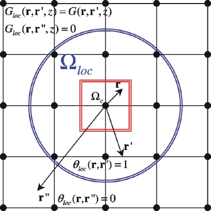
Figure 1: Illustration of the area in real space where the local Green function $G_{loc}$ is defined. Note that $\mathbf{r}$ is restricted by the unit cell at the origin while $\mathbf{r}^{\prime}$ and $\mathbf{r}^{\prime\prime}$ travel within the crystal.

We will now discuss the free energy of a system as a functional of the local Green function.

II.1 Functional of Local Green Function

We consider full many–body Hamiltonian describing the electrons moving in the periodic ionic potential $V_{ext}(x)=V_{ext}(\mathbf{r})\delta(\tau)$ and interacting among themselves according to the Coulomb law: $v_{C}(x-x^{\prime})=e^{2}/|\mathbf{r}-\mathbf{r}^{\prime}|\delta(\tau-\tau^{\prime})$ [we use imaginary time–frequency formalism, where $x=(\mathbf{r},\tau)$]. This is the formal starting point of our all–electron first–principles calculation. So, the theory of everything is summarized in the action $S$:.

$$S=\int dx\psi^{+}(x)[\partial_{\tau}-{\bigtriangledown^{2}}+V_{ext}(x)]\psi(x)$$

$$+{\frac{{1}}{2}}\int dxdx^{\prime}\psi^{+}(x)\psi^{+}(x^{\prime})v_{C}(x-x^{\prime})\psi(x)\psi(x^{\prime})$$ (3)

(atomic Rydberg units, $\hbar=1,m_{e}=1/2$, are used throughout). We will ignore relativistic effects in this action for simplicity but considering our applications to Pu, these effects will be included later in the implementation. In addition, the effects of electron–phonon interaction will not be considered.

We will take the effective action functional approach to describe our correlated system Chitra2 . The approach allows to obtain the free energy of the solid from a functional $\Gamma$ evaluated at its stationary point. The main question is the choice of the variable of the functional which is to be extremized. This question is highly non–trivial because the exact form of the functional is unknown and the usefulness of the approach, depends on our ability to construct good approximations to it, which in turn depends on the choice of variables. The Baym–Kadanoff  (BK) Green function theory considers exact Green function $G(x,x^{\prime})=-\langle T_{\tau}\psi(x)\psi^{+}(x^{\prime})\rangle$ as a variable, i.e. $\Gamma_{BK}[G].$ Density functional theory considers density $\rho(\mathbf{r})=G(\mathbf{r},\mathbf{r},\tau=0)$ of the solid as a variable, i.e. $\Gamma_{DFT}[\rho]$. Spectral density functional theory will consider local Green function $G_{loc}(x,x^{\prime})=$ $G(x,x^{\prime})\theta_{loc}(\mathbf{r},\mathbf{r}^{\prime})$ as a variable, i.e. $\Gamma_{SDF}[G_{loc}].$

Notice on the variety of choices we can make, in particular in the functional $\Gamma_{SDF}[G_{loc}]$ since the definition of the locality is up to us. The usefulness of a given choice is dictated by the existence of good approximations to the functional, as, for example, the usefulness of the DFT is the result of the existence of the LDA or GGA, which are excellent approximations for weakly correlated systems. Here we will argue that the usefulness of SDFT is the existence of the local dynamical mean field approximations.

Any of the discussed functionals can be obtained by a Legendre transform of the effective action. The electronic Green function of a system can be obtained by probing the system by a source field and monitoring the response. To obtain $\Gamma_{BK}[G]$ we probe the system with time–dependent two–variable source field $J(x,x^{\prime})$ or its imaginary frequency transform $J(\mathbf{r},\mathbf{r}^{\prime},i\omega)$ defined in all space. If we restrict our consideration to saddle point solutions periodic on the original lattice, we can assume that the field obeys the periodicity criteria $J(\mathbf{r+R},\mathbf{r}^{\prime}+\mathbf{R},i\omega)=J(\mathbf{r},\mathbf{r}^{\prime},i\omega).$ This restricts the electronic Green function to be invariant under lattice translations. In order to obtain a theory based on the density as a physical variable, we probe the system with a static periodical field $J(\mathbf{r})\delta(\tau).$ This delivers Fukuda ; Makov ; Fernando the density functional theory $\Gamma_{DFT}[\rho]$. In order to obtain $\Gamma_{SDF}[G_{loc}]$ we will probe the system with a local field $J_{loc}(x,x^{\prime})=J_{loc}(\mathbf{r},\mathbf{r}^{\prime},\tau-\tau^{\prime})$ restricted by $\theta_{loc}(\mathbf{r},\mathbf{r}^{\prime}).$

Introduction of the time dependent local source $J_{loc}(x,x^{\prime})$ modifies the action of the system (3) as follows

$$S^{\prime}[J_{loc}]=S+\int dxdx^{\prime}J_{loc}(x,x^{\prime})\psi(x^{\prime})\psi^{+}(x)$$ (4)

Due to translational invariance, the integral over $\mathbf{r}$ variable here is the same for any unit–cell $\Omega_{c}$ and the integral over $\mathbf{r}^{\prime}$ should be restricted by the area where $J_{loc}\neq 0$, i.e. by the cluster area $\Omega_{loc}.$The average of the operator $\psi(x)\psi^{+}(x^{\prime})$ probes the local Green function which is precisely defined by expression (2). The partition function $Z,$ or equivalently the free energy of the system $F,$ becomes a functional of the auxiliary source field

$$Z[J_{loc}]=\exp(-F[J_{loc}])=\int D[\psi^{+}\psi]e^{-S^{\prime}[J_{loc}]}$$ (5)

The effective action for the local Green function, i.e., spectral density functional, is obtained as the Legendre transform of $F$ with respect to the local Green function $G_{loc}(x,x^{\prime})$, i.e.

$$\Gamma_{SDF}[G_{loc}]=F[J_{loc}]-\mathrm{Tr}J_{loc}G_{loc}$$ (6)

where we use the compact notation $\mathrm{Tr}J_{loc}G_{loc}$ for the integrals

$$\mathrm{Tr}J_{loc}G_{loc}=\int dxdx^{\prime}J_{loc}(x,x^{\prime})G_{loc}(x^{\prime},x)=\sum_{i\omega}\int d\mathbf{r}d\mathbf{r}^{\prime}J_{loc}(\mathbf{r},\mathbf{r}^{\prime},i\omega)G_{loc}(\mathbf{r}^{\prime},\mathbf{r},i\omega)$$ (7)

Using the condition: $J_{loc}=-\delta\Gamma_{SDF}/\delta G_{loc}$ to eliminate $J_{loc}$ in (6) in favor of the local Green function we finally obtain the functional of the local Green function alone.

The source field sets the degree of locality of the object of interest. Considering its definition by expanding the cluster till entire solid, we obtain the Baym–Kadanoff functional which determines the Green function in all space. Shrinking its definition to a singe point $\mathbf{r}$ and assuming its frequency (time) independence, i.e. $J(\mathbf{r})\delta(\mathbf{r}-\mathbf{r}^{\prime})\delta(\tau-\tau^{\prime}),$ we obtain density functional theory. In its extremum, all functionals always reach the total free energy of the system regardless the choice of the variable. This situation is similar Makov to classical thermodynamics where the thermodynamic potential is either the Helmholtz free energy, or the Gibs free energy or the entalpy depending on which variables, temperature, pressure, volume are used. Note also that due to assumed time–dependence of the source field, away from the extremum the Green function functionals cannot be interpreted as energies.

Having repeated a formal derivation of the existence Chitra1 of the functional $\Gamma_{SDF}[G_{loc}]$ as well as of the functionals $\Gamma_{BK}[G]$ and $\Gamma_{DFT}[\rho]$ we now come to the problem of writing separately various contributions to it. This development parallels the well known decomposition of the total energy into kinetic energy of a non interacting system, potential energy, Hartree energy and exchange–correlation energy. The strategy consists in performing an expansion of the functional in powers of the charge of the electronChitra1 ; Fukuda ; Fernando ; Antoine1 ; Antoine2 . The lowest order term is the kinetic part of the action, and the energy associated with the external potential $V_{ext}$.  In the Baym Kadanoff Green function theory this term has the form (3):

$$K_{BK}[G]=\mathrm{Tr}\ln G-\mathrm{Tr}[G_{0}^{-1}-G^{-1}]G$$ (8)

The $G_{0}(\mathbf{r},\mathbf{r}^{\prime},i\omega)$ is the non–interacting Green function, which is given by

$$G_{0}^{-1}(\mathbf{r},\mathbf{r}^{\prime},i\omega) = \delta(\mathbf{r}-\mathbf{r}^{\prime})[i\omega+\mu+\nabla^{2}-V_{ext}(\mathbf{r})]$$ (9)

$$\delta(\mathbf{r}-\mathbf{r}^{\prime}) = \int d\mathbf{r}^{\prime\prime}G_{0}^{-1}(\mathbf{r},\mathbf{r}^{\prime\prime},i\omega)G_{0}(\mathbf{r}^{\prime\prime},\mathbf{r}^{\prime},i\omega)$$ (10)

where $\mu$ is a chemical potential. Note that since finite temperature formulation is adopted we did not obtain simply $K_{BK}[G]=\mathrm{Tr(}-\nabla^{2}+V_{ext})G$ but also have got all entropy based contributions.

Let us now turn to the density functional theory. In principle, it does not have a closed formula to describe fully interacting kinetic energy as the density functional. However, it solves this problem by introducing a non–interacting part of the kinetic energy. It is described by its own Green function $G_{KS}(\mathbf{r},\mathbf{r}^{\prime},i\omega),$ which is related to the Kohn–Sham (KS) representation. An auxiliary set of non–interacting particles is introduced which is used to mimic the density of the system. These particles move in some effective one–particle Kohn–Sham potential $V_{eff}(\mathbf{r})=V_{ext}(\mathbf{r})+V_{int}(\mathbf{r})$. This potential is chosen merely to reproduce the density and does not have any other physical meaning at this point. The Kohn–Sham Green function is defined in the entire space by the relation $G_{KS}^{-1}(\mathbf{r},\mathbf{r}^{\prime},i\omega)=G_{0}^{-1}(\mathbf{r},\mathbf{r}^{\prime},i\omega)-V_{int}(\mathbf{r})\delta(\mathbf{r}-\mathbf{r}^{\prime})$, where $V_{int}(\mathbf{r})$ is adjusted so that the density of the system $\rho(\mathbf{r})$ can be found from $G_{KS}(\mathbf{r},\mathbf{r}^{\prime},i\omega)$. Since the exact Green function $G$ and the local Green function $G_{loc}$ can be also used to find the density, we can write a general relationship:

$$\rho(\mathbf{r})=T\sum_{i\omega}G_{KS}(\mathbf{r},\mathbf{r},i\omega)e^{i\omega 0+}=T\sum_{i\omega}G(\mathbf{r},\mathbf{r},i\omega)e^{i\omega 0+}=T\sum_{i\omega}G_{loc}(\mathbf{r},\mathbf{r},i\omega)e^{i\omega 0+}$$ (11)

where the sum over $i\omega$ assumes the summation on the Matsubara axis at given temperature $T$. With the introduction of $G_{KS}$ the non–interacting kinetic portion of the action plus the energy related to $V_{ext}$ can be written in complete analogy with (8) as follows

$$K_{DFT}[G_{KS}]=\mathrm{Tr}\ln G_{KS}-\mathrm{Tr}[G_{0}^{-1}-G_{KS}^{-1}]G_{KS}$$ (12)

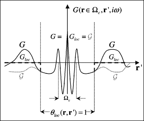
Figure 2: Relationship between various Green functions in spectral density functional theory: exact Green function $G$, local Green function $G_{loc}$ and auxiliary Green function $\mathcal{G}$ are the same in a certain region of space of our interest. They are all different outside this area, where the local Green function is zero by definiton.

In order to describe the different contributions to the thermodynamical potential in the spectral density functional theory, we introduce a notion of the energy–dependent analog of Kohn–Sham representation. These auxiliary particles are interacting so that they will describe not only the density but also a local part of the Green function of the system, and will feel a frequency dependent potential. The latter is a field described by some effective mass operator $\mathcal{M}_{eff}(\mathbf{r},\mathbf{r}^{\prime},i\omega)=V_{ext}(\mathbf{r})\delta(\mathbf{r}-\mathbf{r}^{\prime})+\mathcal{M}_{int}(\mathbf{r},\mathbf{r}^{\prime},i\omega).$ We now introduce an auxiliary Green function $\mathcal{G}(\mathbf{r},\mathbf{r}^{\prime},i\omega)$ connected to our new ”interacting Kohn–Sham” particles so that it is defined in the entire space by the relationship $\mathcal{G}^{-1}(\mathbf{r},\mathbf{r}^{\prime},i\omega)=G_{0}^{-1}(\mathbf{r},\mathbf{r}^{\prime},i\omega)-\mathcal{M}_{int}(\mathbf{r},\mathbf{r}^{\prime},i\omega)$. Thus, $\mathcal{M}_{int}(\mathbf{r},\mathbf{r}^{\prime},i\omega)$ is a function which has the same range as the source that we introduce: it is adjusted until the auxiliary $\mathcal{G}(\mathbf{r},\mathbf{r}^{\prime},i\omega)$ coincides with the local Green function inside the area restricted by $\theta_{loc}(\mathbf{r},\mathbf{r}^{\prime}),$ i.e

$$G_{loc}(\mathbf{r},\mathbf{r}^{\prime},i\omega)=\mathcal{G}(\mathbf{r},\mathbf{r}^{\prime},i\omega)\theta_{loc}(\mathbf{r},\mathbf{r}^{\prime})$$ (13)

We illustrate the relationship between all introduced Green functions in Fig. 2. Note that $\mathcal{G}(\mathbf{r},\mathbf{r}^{\prime},i\omega)$ also delivers the exact density of the system. With the help of $\mathcal{G}$ the kinetic term in the spectral density functional theory can be represented as follows

$$K_{SDF}[\mathcal{G]}=Tr\ln\mathcal{G}-Tr[G_{0}^{-1}-\mathcal{G}^{-1}]\mathcal{G}$$ (14)

Since $G_{KS}$ is a functional of $\rho$, DFT considers the density functional as the functional of Kohn–Sham wave functions, i.e. as $\Gamma_{DFT}[G_{KS}].$ Similarly, since $\mathcal{G}$ is a functional of $G_{loc}$, it is very useful to view the spectral density functional $\Gamma_{SDF}$ as a functional of $\mathcal{G}$:

$$\Gamma_{SDF}[\mathcal{G}]=\mathrm{Tr}\ln\mathcal{G}-\mathrm{Tr}[G_{0}^{-1}-\mathcal{G}^{-1}]\mathcal{G}+\Phi_{SDF}[G_{loc}]$$ (15)

where the unknown interaction part of the free energy $\Phi_{SDF}[G_{loc}]$ is the functional of $G_{loc}.$ If the Hartree term is explicitly extracted, this functional can be represented as

$$\Phi_{SDF}[G_{loc}]=E_{H}[\rho]+\Phi_{SDF}^{xc}[G_{loc}]$$ (16)

where $E_{H}[\rho]$ is the Hartree energy depending only on the density of the system, and where $\Phi_{SDF}^{xc}[G_{loc}]$ is the exchange–correlation part of the free energy. Notice that the density of the system can be obtained via $G_{loc}$ or $\mathcal{G},$ therefore the Hartree term can be also viewed as a functional of $G_{loc}$ or $\mathcal{G}.$ Notice also, that since the kinetic energies (8), (12), (14) are defined differently in all theories, the interaction energies $\Phi_{SDF}[G_{loc}],$ $\Phi_{BK}[G],$ $\Phi_{DFT}[\rho]$ are also different.

The stationarity of the spectral density functional can be examined with respect to $\mathcal{G}$

$$\frac{\delta\Gamma_{SDF}}{\delta\mathcal{G}(\mathbf{r},\mathbf{r}^{\prime},i\omega)}=0$$ (17)

similar to the stationarity conditions for $\Gamma_{BK}[G]$ and $\Gamma_{DFT}[G_{KS}]$

$$\frac{\delta\Gamma_{BK}}{\delta G(\mathbf{r},\mathbf{r}^{\prime},i\omega)} = 0$$ (18)

$$\frac{\delta\Gamma_{DFT}}{\delta G_{KS}(\mathbf{r},\mathbf{r}^{\prime},i\omega)} = 0$$ (19)

This leads to the equations for the corresponding Green functions in all theories:

$$\mathcal{G}^{-1}(\mathbf{r},\mathbf{r}^{\prime},i\omega)=G_{0}^{-1}(\mathbf{r},\mathbf{r}^{\prime},i\omega)-\mathcal{M}_{int}(\mathbf{r},\mathbf{r}^{\prime},i\omega)$$ (20)

as well as

$$G^{-1}(\mathbf{r},\mathbf{r}^{\prime},i\omega) = G_{0}^{-1}(\mathbf{r},\mathbf{r}^{\prime},i\omega)-\Sigma_{int}(\mathbf{r},\mathbf{r}^{\prime},i\omega)$$ (21)

$$G_{KS}^{-1}(\mathbf{r},\mathbf{r}^{\prime},i\omega) = G_{0}^{-1}(\mathbf{r},\mathbf{r}^{\prime},i\omega)-V_{int}(\mathbf{r})\delta(\mathbf{r}-\mathbf{r}^{\prime})$$ (22)

By using (9) for $G_{0}^{-1}$ and by multiplying both parts by the corresponding Green functions we obtain familiar Dyson equations

$$[-\nabla^{2}+V_{ext}(\mathbf{r})-i\omega-\mu]\mathcal{G}(\mathbf{r},\mathbf{r}^{\prime},i\omega)+\int d\mathbf{r}^{\prime\prime}\mathcal{M}_{int}(\mathbf{r},\mathbf{r}^{\prime\prime},i\omega)\mathcal{G}(\mathbf{r}^{\prime\prime},\mathbf{r}^{\prime},i\omega)=\delta(\mathbf{r}-\mathbf{r}^{\prime})$$ (23)

and

$$[-\nabla^{2}+V_{ext}(\mathbf{r})-i\omega-\mu]G(\mathbf{r},\mathbf{r}^{\prime},i\omega)+\int d\mathbf{r}^{\prime\prime}\Sigma_{int}(\mathbf{r},\mathbf{r}^{\prime\prime},i\omega)G(\mathbf{r}^{\prime\prime},\mathbf{r}^{\prime},i\omega) = \delta(\mathbf{r}-\mathbf{r}^{\prime})$$ (24)

$$[-\nabla^{2}+V_{ext}(\mathbf{r})-i\omega-\mu]G_{KS}(\mathbf{r},\mathbf{r}^{\prime},i\omega)+V_{int}(\mathbf{r})G_{KS}(\mathbf{r}^{\prime\prime},\mathbf{r}^{\prime},i\omega) = \delta(\mathbf{r}-\mathbf{r}^{\prime})$$ (25)

The stationarity condition brings the definition of the auxiliary mass operator $\mathcal{M}_{int}(\mathbf{r},\mathbf{r}^{\prime},i\omega)$ which is the variational derivative of the interaction free energy with respect to the local Green function:

$$\mathcal{M}_{int}(\mathbf{r},\mathbf{r}^{\prime},i\omega)=\frac{\delta\Phi_{SDF}[G_{loc}]}{\delta\mathcal{G}(\mathbf{r}^{\prime},\mathbf{r},i\omega)}=\frac{\delta\Phi_{SDF}[G_{loc}]}{\delta G_{loc}(\mathbf{r}^{\prime},\mathbf{r},i\omega)}\theta_{loc}(\mathbf{r},\mathbf{r}^{\prime})$$ (26)

It plays the role of the effective self–energy which is short–ranged (local) in the space. The corresponding expressions hold for the interaction parts of the exact self–energy of the electron $\Sigma_{int}(\mathbf{r},\mathbf{r}^{\prime},i\omega)$ and for the interaction part of the Kohn–Sham potential $V_{int}(\mathbf{r}).$

$$\Sigma_{int}(\mathbf{r},\mathbf{r}^{\prime},i\omega) = \frac{\delta\Phi_{BK}[G]}{\delta G(\mathbf{r}^{\prime},\mathbf{r},i\omega)}$$ (27)

$$V_{int}(\mathbf{r})\delta(\mathbf{r}-\mathbf{r}^{\prime}) = \frac{\delta\Phi_{DFT}[\rho]}{\delta G_{KS}(\mathbf{r}^{\prime},\mathbf{r},i\omega)}=\frac{\delta\Phi_{DFT}[\rho]}{\delta\rho(\mathbf{r})}\delta(\mathbf{r}-\mathbf{r}^{\prime})$$ (28)

If the external potential is added to these quantities we obtain total effective self–energies/potentials of the SDF, BK and DF theories: $\mathcal{M}_{eff}(\mathbf{r},\mathbf{r}^{\prime},i\omega),$ $\Sigma_{eff}(\mathbf{r},\mathbf{r}^{\prime},i\omega),$ $V_{eff}(\mathbf{r})$ respectively. If the Hartree potential $V_{H}(\mathbf{r})$ is separated we obtain the exchange–correlation parts: $\mathcal{M}_{xc}(\mathbf{r},\mathbf{r}^{\prime},i\omega),$ $\Sigma_{xc}(\mathbf{r},\mathbf{r}^{\prime},i\omega),$ $V_{xc}(\mathbf{r}).$

Note that strictly speaking the substitution of variables, $G_{KS}$ vs. $\rho,$ in the density functional as well as the substitution of variables, $\mathcal{G}$ vs. $G_{loc}$, in the spectral density functional is only possible under the assumption of the so–called $V$–representability (or $M$–representability), i.e. the existence of such effective potential (mass operator) which can be used to construct the exact density (local Green function) of the system via the non–interacting Kohn–Sham particles of the DFT or its energy–dependent generalization in SDFT.

Note also that the effective mass–operator of spectral density functional theory is local by construction, i.e. it is non–zero only within the cluster area $\Omega_{loc}$ restricted by $\theta_{loc}(\mathbf{r},\mathbf{r}^{\prime}).$ It is an auxiliary object which cannot be identified with the exact self–energy of the electron $\Sigma_{eff}(\mathbf{r},\mathbf{r}^{\prime},i\omega).$ This is similar to the observation that the Kohn–Sham potential of the DFT cannot be associated with the exact self–energy as well. Nevertheless, the SDFT always delivers local Green function and the total free energy exactly (at least in principle) as long as the exact functional is used. In the limit when the exact self–energy of the electron is indeed localized within $\Omega_{loc}$, the SDFT becomes the Baym–Kadanoff functional which delivers the full Green function of the system, i.e. we can immediately identify $\mathcal{M}_{eff}(\mathbf{r},\mathbf{r}^{\prime},i\omega)$ with $\Sigma_{eff}(\mathbf{r},\mathbf{r}^{\prime},i\omega)$ and the poles of $\mathcal{G}(\mathbf{r},\mathbf{r}^{\prime},i\omega)$ with exact poles of $G(\mathbf{r},\mathbf{r}^{\prime},i\omega)$ where the information about both k and energy dependence as well as life time of the quasiparticles is contained. We thus see that, at least formally, increasing the size of $\Omega_{loc}$  in the SDF theory leads to a complete description of the many–body system, the situation quite different from the DFT which misses such scaling.

From a conceptual point of view, the spectral density functional approach constitutes a radical departure from the DFT philosophy. The saddle–point equation (23) is the equation for a continuous distribution of spectral weight and the obtained local spectral function $G_{loc}$ can now be identified with the observable local (roughly speaking, k–integrated) one–electron spectrum. This is very different from the Kohn–Sham quasiparticles which are the poles of $G_{KS}$ not identifiable rigorously with any one–electron excitations. While the SDFT approach is computationally more demanding than DFT, it is formulated in terms of observables and gives more information than DFT.

On one side, spectral density functional can be viewed as approximation or truncation of the full Baym Kadanoff theory where $\Phi_{BK}[G]$ is approximated by $\Phi_{SDF}[G_{loc}]$  by restricting  $G$ to $G_{loc}$Chitra2 and the kinetic functionals $K_{BK\text{ }}[G]$ and $K_{SDF}[\mathcal{G}]$ are thought to be the same. Such restriction will automatically generate a short–ranged self–energy in the theory. This is similar to the interpretation of DFT as approximation $\Phi_{BK}[G]=\Phi_{DFT}[\rho],K_{BK\text{ }}[G]$=$K_{SDF}[G_{KS}]$ which would generate the DFT potential as the self–energy. However, SDFT can be thought as a separate theory whose manifestly local self–energy is an auxiliary operator introduced to reproduce the local part of the Green function of the system, exactly like the Kohn–Sham ground state potential is an auxiliary operator introduced to reproduce the density of the electrons in DFT.

Spectral density functional theory contains the exchange–correlation functional $\Phi_{SDF}[G_{loc}]$. An explicit expression for it involving a coupling constant $\lambda=e^{2}$  integration can be obtained in complete analogy with the Harris–Jones formulaHarris of density functional theoryAntoine2 . One considers $\Gamma_{SDF}[\mathcal{G},\lambda]$ at an arbitrary interaction $\lambda$ and expresses

$$\Gamma_{SDF}[\mathcal{G},e^{2}]=\Gamma_{SDF}[\mathcal{G},0]+\int_{0}^{e^{2}}d\lambda\frac{\partial\Gamma_{SDF}[\mathcal{G},\lambda]}{\partial\lambda}$$ (29)

Here the first term is simply the kinetic part $K_{SDF}[\mathcal{G]}$ as given by (14) which does not depend on $\lambda$. The second part is thus the unknown functional $\Phi_{SDF}[G_{loc}].$ The derivative with respect to the coupling constant in (3)  is given by the average $\langle\psi^{+}(x)\psi^{+}(x^{\prime})\psi(x)\psi(x^{\prime})\rangle$ $=\Pi_{\lambda}(x,x^{\prime},i\omega)+$ $\langle\psi^{+}(x)\psi(x)\rangle\langle\psi^{+}(x^{\prime})\psi(x^{\prime})\rangle$ where $\Pi_{\lambda}(x,x^{\prime})$ is the density–density correlation function at a given interaction strength $\lambda$ computed in the presence of a source which is $\lambda$ dependent  and chosen so that the local Greens function of the system is $\mathcal{G}$. Since $\langle\psi^{+}(x)\psi(x)\rangle=\rho(\mathbf{r})\delta(\tau),$ we can obtain :

$$\Phi_{SDF}[G_{loc}]=E_{H}[\rho]+\sum_{i\omega}\int_{0}^{e^{2}}d\lambda\frac{\Pi_{\lambda}(\mathbf{r},\mathbf{r}^{\prime},i\omega)}{|\mathbf{r}-\mathbf{r}^{\prime}|}$$ (30)

Establishing the diagrammatic rules for the functional $\Phi_{SDF}[G_{loc}]$ while possible Chitra1 , is not as simple as for the functional $\Phi_{BK}[G].$ The latter is formally represented as a sum of two–particle diagrams constructed with $G$ and $v_{C}.$ It is well known that instead of expanding $\Phi_{BK}[G]$ in powers of the bare interaction $v_{C}$ and $G,$ the functional form can be obtained by introducing the dynamically screened Coulomb interaction $W(\mathbf{r},\mathbf{r}^{\prime},i\omega)$ as a variable. In the effective action formalism Chitra2 this was done by introducing an auxiliary Bose variable coupled to the density, which transforms the original problem into a problem of electrons interacting with the Bose field. $W$ is the connected correlation function of the Bose field.

Our effective action is now a functional of $G$, $W$ and of the expectation value of the Bose field. Since the latter couples linearly to the density it can be eliminated exactly, a step which generates the Hartree term. After this elimination, the functional takes the form

$$\Gamma_{BK}[G,W]=\mathrm{Tr}\ln G-\mathrm{Tr}[G_{0}^{-1}-G^{-1}]G+\Phi_{BK}[G,W]$$ (31)

$$\Phi_{BK}[G,W]=E_{H}[\rho]-\frac{1}{2}\mathrm{Tr}\ln W+\frac{1}{2}\mathrm{Tr}[v_{C}^{-1}-W^{-1}]W+\Psi_{BK}[G,W]$$ (32)

The entire theory is viewed as the functional of both $G$ and $W.$ Here, $\Psi_{BK}[G,W]$ is the sum of all two–particle diagrams constructed with $G$ and $W$ with the exclusion of the Hartree term, which is evaluated with the bare Coulomb interaction. An additional stationarity condition $\delta\Gamma_{BK}/\delta W=0$ leads to the equation for the screened Coulomb interaction $W$

$$W^{-1}(\mathbf{r},\mathbf{r}^{\prime},i\omega)=v_{C}^{-1}(\mathbf{r}-\mathbf{r}^{\prime})-\Pi(\mathbf{r},\mathbf{r}^{\prime},i\omega)$$ (33)

where the function $\Pi(\mathbf{r},\mathbf{r}^{\prime},i\omega)=-2\delta\Psi_{BK}/\delta W(\mathbf{r},\mathbf{r}^{\prime},i\omega)$ is the exact interacting susceptibility of the system, which is already discussed in connection with representation (30).

A similar theory is developed for the local quantities Chitra2 , and this generalization represents the ideas of extended dynamical mean field theory EDMFT , now viewed as an exact theory. Namely, one constructs an exact functional of the local Greens function and the local correlator of the Bose field coupled to the density which can be identified with the local part of the dynamically screened interaction. The real–space definition of it is the following

$$W_{loc}(\mathbf{r},\mathbf{r}^{\prime},i\omega)=W(\mathbf{r},\mathbf{r}^{\prime},i\omega)\theta_{loc}(\mathbf{r},\mathbf{r}^{\prime})$$ (34)

which is non–zero within a given cluster $\Omega_{loc}$. Note that formally this cluster can be different from the one considered to define the local Green function (2) but we will not distinguish between them for simplicity. An auxiliary interaction $\mathcal{W}(\mathbf{r},\mathbf{r}^{\prime},i\omega)$ is introduced which is the same as the local part of the exact interaction within non–zero area of $\theta_{loc}(\mathbf{r},\mathbf{r}^{\prime})$

$$W_{loc}(\mathbf{r},\mathbf{r}^{\prime},i\omega)=\mathcal{W}(\mathbf{r},\mathbf{r}^{\prime},i\omega)\theta_{loc}(\mathbf{r},\mathbf{r}^{\prime})$$ (35)

The interaction part of the spectral density functional is represented in the form similar to (32)

$$\Phi_{SDF}[G_{loc},W_{loc}]=E_{H}[\rho]-\frac{1}{2}\mathrm{Tr}\ln\mathcal{W}+\frac{1}{2}\mathrm{Tr}[v_{C}^{-1}-\mathcal{W}^{-1}]\mathcal{W}+\Psi_{SDF}[G_{loc},W_{loc}]$$ (36)

and the spectral density functional is viewed as a functional $\Gamma_{SDF}[G_{loc},W_{loc}]$ or alternatively as a functional $\Gamma_{SDF}[\mathcal{G},\mathcal{W}]$. $\Psi_{SDF}[G_{loc},W_{loc}]$ is formally not a sum of two–particle diagrams constructed with $G_{loc}\$and $W_{loc}$, but in principle a more complicated diagrammatic expression can be derived. Alternatively, a more explicit expression involving a coupling constant integration can be given. Examining stationarity $\delta\Gamma_{SDF}/\delta\mathcal{W}=0$ yields a saddle–point equation for $\mathcal{W}(\mathbf{r},\mathbf{r}^{\prime},i\omega)$

$$\mathcal{W}^{-1}(\mathbf{r},\mathbf{r}^{\prime},i\omega)=v_{C}^{-1}(\mathbf{r}-\mathbf{r}^{\prime})-\mathcal{P}(\mathbf{r},\mathbf{r}^{\prime},i\omega)$$ (37)

where the effective susceptibility of the system is the variational derivative

$$\mathcal{P}(\mathbf{r},\mathbf{r}^{\prime},i\omega)=\frac{-2\delta\Psi_{SDF}}{\delta\mathcal{W}(\mathbf{r}^{\prime},\mathbf{r},i\omega)}=\frac{-2\delta\Psi_{SDF}}{\delta W_{loc}(\mathbf{r}^{\prime},\mathbf{r},i\omega)}\theta_{loc}(\mathbf{r},\mathbf{r}^{\prime})$$ (38)

Notice again a set of parallel observations for $\mathcal{P}$ as for $\mathcal{M}_{eff}$, Eq. (26). The effective susceptibility of spectral density functional theory is local by construction, i.e. it is non–zero only within the cluster restricted by $\theta_{loc}(\mathbf{r},\mathbf{r}^{\prime}).$ Formally, it is an auxiliary object and cannot be identified with the exact susceptibility of the electronic system $\Pi(\mathbf{r},\mathbf{r}^{\prime},i\omega).$ However, if the exact susceptibility $\Pi(\mathbf{r},\mathbf{r}^{\prime},i\omega)$ is sufficiently localized, this identification becomes possible. If cluster $\Omega_{loc}$ includes physical area of localization, we can immediately identify $\mathcal{P}(\mathbf{r},\mathbf{r}^{\prime},i\omega)$ with $\Pi(\mathbf{r},\mathbf{r}^{\prime},i\omega)$ and $\mathcal{W}(\mathbf{r},\mathbf{r}^{\prime},i\omega)$ with $W(\mathbf{r},\mathbf{r}^{\prime},i\omega)$ in all space. However, both $\mathcal{W}$ and $W$ are always the same within $\Omega_{loc}$ regardless its size, as it is seen from (34) and (35).

At the stationarity point, $\Gamma_{SDF}[\mathcal{G},\mathcal{W}]$ is the free energy $F$ of the system. If one inserts (20) into (14) and (37) into (36) we obtain the formula:

$$F=\mathrm{Tr}\ln\mathcal{G}-\mathrm{Tr}\mathcal{M}_{eff}\mathcal{G}+\mathrm{Tr}V_{ext}\mathcal{G+}E_{H}-\frac{1}{2}\mathrm{Tr}\ln\mathcal{W}+\frac{1}{2}\mathrm{Tr}\mathcal{PW}+\Psi_{SDF}$$ (39)

Similar formulae hold for the Baym–Kadanoff and density functional theories

$$F = \mathrm{Tr}\ln G-\mathrm{Tr}\Sigma_{eff}G+\mathrm{Tr}V_{ext}G+E_{H}-\frac{1}{2}\mathrm{Tr}\ln W+\frac{1}{2}\mathrm{Tr}\Pi W+\Psi_{BK}$$ (40)

$$F = \mathrm{Tr}\ln G_{KS}-\mathrm{Tr}V_{eff}G_{KS}+\mathrm{Tr}V_{ext}G_{KS}+\Phi_{DFT}$$ (41)

where the first two terms in all expressions (39), (40), (41) are interpreted as corresponding kinetic energies, the third term is the energy related to the external potential $V_{ext}$ which is in fact $\mathrm{Tr}V_{ext}\rho$ in all cases. The other terms represent the interaction parts of the free energy. Note that all entropy originated contributions are included in both kinetic and interaction parts. If temperature goes to zero, the entropy part disappears and the total energy formulae will be recovered. For example, in spectral density functional theory we obtain:

$$E=-\mathrm{Tr}\nabla^{2}\mathcal{G}+\mathrm{Tr}V_{ext}\rho+E_{H}+\Phi_{xc}$$ (42)

We will also discuss this limit later in more details in Section III.

The SDFT approach is so far not very useful since a tractable expression for the functional form of $\Phi_{SDF}[G_{loc}]$ or $\Psi_{SDF}[G_{loc},W_{loc}]$ has not been given yet. This is quite similar to the unknown exchange–correlation functional of the DFT. As we have learned from the developments of the dynamical mean–field methods, a very useful approximation exists to access these functionals. This is based on a full many–body solution of a finite–size cluster problem treated as an impurity embedded into a bath subjected to a self–consistency condition. Such local dynamical mean field theory will be discussed below.

II.2 Local Dynamical Mean Field Approximation

The spectral density functional theory, where an exact functional of  certain local quantities is constructed in the spirit of Ref. Chitra1, uses effective self–energies and susceptibilities which are local by construction. This property can be exploited to find good approximations to the interaction energy functional. For example, if it is a priori known that the real electronic self–energy is local in a certain portion of the Hilbert space, a good approximation is the corresponding local dynamical mean field theory obtained for example by a restriction or truncation of the full Baym–Kadanoff functional or its generalization to use $W$ and $G$ as natural variables, to local quantities in the spirit of Ref. Chitra2, .

The local DMFT approximates the functional $\Phi_{SDF}[G_{loc}]$ (or $\Psi_{SDF}[G_{loc},W_{loc}])$ by the sum of all two–particle diagrams evaluated with $G_{loc}$ and the bare Coulomb interaction $v_{C}$ (or screened local interaction $W_{loc}).$ In other words, the functional dependence of the interaction part $\Phi_{BK}[G]$ in the Baym–Kadanoff functional for which the diagrammatic rules exist is now restricted by $G_{loc}$ and is used as an approximation to $\Phi_{SDF}[G_{loc}]$, i.e. $\Phi_{SDF}[G_{loc}]=\Phi_{BK}[G_{loc}].$ Obviously that the variational derivative of such restricted functional will generate the self–energy confined in the same area as the local Green function itself.

Remarkably the summation over all local diagrams can be performed exactly via introduction of an auxiliary quantum impurity model subjected to a self–consistency condition Georges92 ; ReviewDMFT . If this impurity is considered as a cluster $C$, the cellular DMFT (C–DMFT) can be used which breaks the translational invariance of the lattice to obtain accurate estimates of the self energies. The C–DMFT approximation, can also be motivated using the cavity construction. The solid should be separated onto large cells which circumscribe the areas $\Omega_{loc}$. Considering the effective action $S,$ Eq. (3), the integration volume is separated onto the cellular area $\Omega_{C}$ and the rest bath area $\Omega-\Omega_{C}=\Omega_{bath}.$ The action is now represented as the action of the cluster cell, $\Omega_{C}$ plus the action of the bath,$\ \Omega_{bath},\$plus the interaction between those two. We are interested in the local effective action $S_{C}$ of the cluster degrees of freedom only, which is obtained conceptually by integrating out the bath in the functional integral:

$$\frac{1}{Z_{C}}\exp[-S_{C}]=\frac{1}{Z}\int_{\Omega_{bath}}d\mathbf{r}d\mathbf{r}^{\prime}\exp[-S]$$ (43)

where $Z_{C}$ and $Z$ are the corresponding partition functions. This integration  is carried out approximately, keeping only a charge–charge interaction as quartic terms and neglecting all the higher order terms generated in this process to arrive to a cavity action of the form EDMFT ; Chitra2 ; CDMFT ; Ping :

$$S_{C}=-\int dx\psi^{+}(x)\mathcal{G}_{0}^{-1}(x,x^{\prime})\psi(x^{\prime})$$

$$+{\frac{{1}}{2}}\int dxdx^{\prime}\psi^{+}(x)\psi^{+}(x^{\prime})\mathcal{V}_{0}(x,x^{\prime})\psi(x)\psi(x^{\prime})$$ (44)

where the integration over the spatial variables is performed over $\Omega_{C}.$ Here $\mathcal{G}_{0}(x,x^{\prime})$ or its Fourier transform $\mathcal{G}_{0}(\mathbf{r},\mathbf{r}^{\prime},i\omega)$ is identified as the bath Green function appeared in the Dyson equation for the local mass operator $\mathcal{M}_{int}(\mathbf{r},\mathbf{r}^{\prime},i\omega)$ and for the local Green function $G_{loc}(\mathbf{r},\mathbf{r}^{\prime},i\omega)$ of the cluster, and $\mathcal{V}_{0}(\mathbf{r},\mathbf{r}^{\prime},i\omega)$ is the ”bath interaction” appeared in the Dyson equation for the local susceptibility $\mathcal{P}(\mathbf{r},\mathbf{r}^{\prime},i\omega)$ and local interaction $W_{loc}(\mathbf{r},\mathbf{r}^{\prime},i\omega),$ i.e

$$\mathcal{G}_{0}^{-1}(\mathbf{r},\mathbf{r}^{\prime},i\omega) = G_{loc}^{-1}(\mathbf{r},\mathbf{r}^{\prime},i\omega)+\mathcal{M}_{int}(\mathbf{r},\mathbf{r}^{\prime},i\omega)$$ (45)

$$\mathcal{V}_{0}^{-1}(\mathbf{r},\mathbf{r}^{\prime},i\omega) = W_{loc}^{-1}(\mathbf{r},\mathbf{r}^{\prime},i\omega)+\mathcal{P}(\mathbf{r},\mathbf{r}^{\prime},i\omega)$$ (46)

Note that neither $\mathcal{G}_{0}$ nor $\mathcal{V}_{0}$ can be associated with non–interacting $G_{0}$ and bare interaction $v_{C},$ respectively. Note also that both $\mathbf{r}$ and $\mathbf{r}^{\prime}$ indexes in $\mathcal{G}_{0}(\mathbf{r},\mathbf{r}^{\prime},i\omega)$ and in $\mathcal{V}_{0}(\mathbf{r},\mathbf{r}^{\prime},i\omega)$ vary within the cellular area $\Omega_{C}.$ The same should be assumed for the local quantities $G_{loc}(\mathbf{r},\mathbf{r}^{\prime},i\omega)$ and $W_{loc}(\mathbf{r},\mathbf{r}^{\prime},i\omega).$ Since these functions are translationally invariant on the original lattice, this property can be used to set up these functions within $\Omega_{C}.$

An interesting observation can be made on the role of the impurity model which in the present context appeared as an approximate way to extract the self–energy of the lattice using input bath Green function and bath interaction. Alternatively, the impurity problem can be thought itself as the model which delivers exact mass operator of the spectral density functional Chitra1 . If the latter is known, there should exist such bath Green function and such bath interaction which can be used to reproduce it. In this respect, the local interaction $W_{loc}$ appeared in our formulation can be thought as an exact way to define the local Coulomb repulsion ”$U$”, i.e. such interaction which delivers exact local self–energy.

To summarize, the effective action for the cluster cell (44), the Dyson equations (45), (46) connecting local and bath quantities as well as the original Dyson equations (20), (37) constitute a self–consistent set of equations as the saddle–point conditions extremizing the spectral density functional $\Gamma_{SDF}(\mathcal{G},\mathcal{W})$. They combine cellular and extended versions of DMFT and represent our philosophy in the ab initio simulation of a strongly correlated system. Since $\mathcal{M}_{int}$ and $\mathcal{P}$ are unknown at the beginning, the solution of these equations assumes self–consistency. First, assuming some initial $\mathcal{M}_{int},$and $\mathcal{P}$ the original Dyson equations (20), (37) are used to find Green function $\mathcal{G}$ and screened interaction $\mathcal{W}.$ Second, the Dyson equations for the local quantities (45), (46) are used to find $\mathcal{G}_{0}$, $\mathcal{V}_{0}.$ Third, quantum impurity model with the cluster action $S_{loc}$ after (44) is solved by available many–body technique to give new local $\mathcal{M}_{int}$ and $\mathcal{P}$. The process is repeated till self–consistency is reached. This is schematically illustrated in Fig. 3. Note here that while single–site impurity problem has a well–defined algorithm to extract the lattice self–energy, this is not generally true for the cluster impurity models Biroli . The latter provides the self–energy of the cluster, and an additional prescription such as implemented within cellular DMFT or using DCA should be given to construct the self–energy of the lattice.

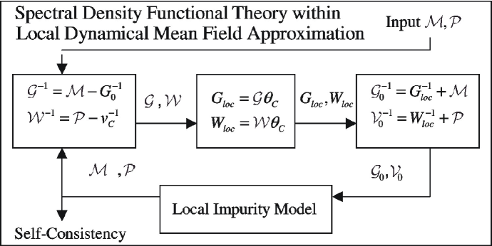
Figure 3: Illustration of self-consistent cycle in spectral density functional theory with local dynamical mean-field approximation: both local Green function $G_{loc}$ and local Coulomb interaction $W_{loc}$ are iterated. The auxiliary quantities $\mathcal{G}$ and $\mathcal{W}$ are used to simplify the construction of the functional.

Unfortunately, writing down the precise functional form for $\Phi_{SDF}[G_{loc},W_{loc}]$ or $\Psi_{SDF}[G_{loc},W_{loc}]$ is still a problem because the evaluation of the entropy requires the evaluation of the energy as a function of temperature and an additional integration over it. In general, the free energy $F=E-TS,$ where $E$ is the total energy and $S$ is the entropy. Since $\Gamma_{SDF}[\mathcal{G}]=K_{SDF}[\mathcal{G}]+\Phi_{SDF}[G_{loc}],$ both energy and entropy terms exist in the kinetic and interaction functionals. The energy part of $K_{SDF}[\mathcal{G}]=\mathrm{Tr(}-\nabla^{2}+V_{ext})\mathcal{G}\$and the energy part of $\Phi_{SDF}[G_{loc},W_{loc}]$ can be written explicitly as $\frac{1}{2}\mathrm{Tr}\mathcal{M}_{int}G_{loc}.$ The entropy correction is a more difficult one. In principle, it can be evaluated by performing calculations of the total energy $E_{SDF}[\mathcal{G}]=\mathrm{Tr(}-\nabla^{2}+V_{ext})\mathcal{G}+\frac{1}{2}\mathrm{Tr}\mathcal{M}_{int}G_{loc}$ at several temperatures and then taking the integral ReviewDMFT :

$$S(T)=S(\infty)-\int_{T}^{\infty}dT^{\prime}\frac{1}{T^{\prime}}\frac{dE_{SDF}}{dT^{\prime}}$$ (47)

The infinite temperature limit $S(\infty)$ for a well defined model Hamiltonian can be worked out. This program was implemented for the Hubbard model Marcelo and for Ce CeMcMahan .

Two well separate problems are now seen. For a given material using the formulae (20), (37), (2), (34), (45), (46) $\mathcal{G},\mathcal{W},G_{loc},W_{loc},\mathcal{G}_{0},\mathcal{V}_{0}$ should be computed using the methods and algorithms of the electronic structure theory. This procedure will in part be described in Section III. With given input $\mathcal{G}_{0}$ and $\mathcal{V}_{0},$ the solution of the impurity model constitutes a well separated problem which can be carried out either using the QMC method or other impurity solver. Some of the techniques are discussed in Refs. ReviewDMFT, ; ReviewLDA+DMFT, . In Section IV, while applying a simplified version of the theory to plutonium, we will briefly describe an impurity solver used in that calculation. A full description of this method will appear elsewhere Udo .

The described algorithm is quite general, totally ab initio and allows to determine all quantities, such as the one–electron local Green functions $G_{loc}$ and the dynamically screened local interactions $W_{loc}$. Unfortunately, its full implementation is a very challenging project which so far has only been carried out at the level of model HamiltoniansPing . There are several simplifications which can be made, however. The screened Coulomb interaction $\mathcal{W}(\mathbf{r},\mathbf{r}^{\prime},i\omega)$ can be treated on different levels of approximations. In many cases used in practical calculations with the LDA+DMFT method, this interaction $\mathcal{W}$ is assumed to be static and parametrized by a set of some optimally screened on–site parameters, such as Hubbard $U$ and exchange $J$. These parameters can be fixed by constrained density functional calculations, extracted from atomic spectra data or adjusted to fit the experiment. Since the described theory can perform a search in a constrained space with fixed interaction $\mathcal{W},$ this justifies the use of $U$ and $J$ as input numbers. A more refined approximation, can use a method such as GW to generate an energy–dependent $\mathcal{W}$ Ferdi which is then treated using extended DMFT Ping . Alternatively we can envision that $\mathcal{W}$ is already so short ranged that we can ignore the EDMFT self consistency condition, and we treat $\mathcal{W}$ as $\mathcal{W}_{fix}(x,x^{\prime})$ .This leads to performing a partial self–consistency with respect to the Green function only. The procedure is reduced to solving Dyson equations (20), (45) as well as to finding $\mathcal{M}_{int}$ via the solution of the impurity problem. A full self–consistency can finally be restored by including a second loop to relax $\mathcal{W}.$

A methodological comment should be made in order to make contact with the literature of cluster extensions of single site DMFT within model Hamiltonians. We adopted a less restrictive notion of locality by defining an effective action of the one particle Green function (and of the interaction) whose arguments are in nearby unit cells. This maintains the full translation invariance of the lattice. At the level of the exact effective action , this is an exact construction, and its extremization will lead to portions of the exact Greens function which obeys causality. Notice however that it has been proved recentlyBiroli  that generating approximations to the exact functional by restricting the Baym Kadanoff functional to non local Greens functions leads to violations of causality. For this reason, we propose to use techniques such as CDMFT which are manifestly causal for the purpose of realizing approximations to the local Greens functions.

Our final general comment concerns the optimal choice of local representation or, precisely, the definition of the local Green function. This is because the local dynamical mean–field approximation is likely to be accurate only  if we know in which portion of the Hilbert space the real electronic self–energy is well localized. Unfortunately, this is not known a priori, and in principle, only a full cluster DMFT calculation is capable to provide us some hints in attempts to answer this question. However, considerable empirical evidence can be used as a guide for choosing a basis for DMFT calculations, and we discuss these issues in the following sections.

II.3 Choice of Local Representation

We have already pointed out that spectral density functional theory is a basis set dependent theory since it probes the Green function locally in a certain region determined by a choice of basis functions in the Hilbert space. Provided the calculation is exact, the free energy of the system and the local spectral density in that Hilbert space will be recovered regardless the choice of it. We have developed the theory assuming that the basis in the Hilbert space is indeed the real space which gives us the choice (2) for the local Green function, i.e. the part of the real Green function restricted by $\theta_{loc}(\mathbf{r},\mathbf{r}^{\prime}).$ While this is most natural choice for the purpose of formulating locality in $\mathbf{r}$ and $\mathbf{r}^{\prime}$ variables, it is also very useful to discuss a more general choice, connected to some space of orbitals $\chi_{\xi}(\mathbf{r})$ which can be used to represent all the relevant quantities in our calculation. As we have in mind to utilize sophisticated basis sets of modern electronic structure calculations, we will sometimes waive the orthogonality condition and will introduce the overlap matrix $O_{\xi\xi^{\prime}}=\langle\chi_{\xi}|\chi_{\xi^{\prime}}\rangle$ especially in cases when we discuss a practical implementation of the method.

We note that the space $\chi_{\xi}(\mathbf{r})$ can in principle be interpreted as the reciprocal space plane wave representation $\chi_{\xi}(\mathbf{r})=e^{i(\mathbf{k}+\mathbf{G})\mathbf{r}},\xi=\mathbf{k}+\mathbf{G}$ with $\mathbf{k}$ being the Brillouin zone vector and $\mathbf{G}$ being the reciprocal lattice vector. Thus the Green function can be probed in the region of the reciprocal space. It can be interpreted as the real space representation if $\chi_{\xi}(\mathbf{r})=\delta(\mathbf{\xi}-\mathbf{r})$ where the sums over $\xi$ are interpreted as the integrals over the volume, and the locality in this basis is precisely exploited in (2). A tremendous transparency of the theory will also arrive if we interpret the orbital space $\{\chi_{\xi}\}$ as a general non–orthogonal tight-binding basis set when index $\xi$ combines the angular momentum index $lm$, and the unit cell index $\mathbf{R},$ i.e. $\chi_{\xi}(\mathbf{r})=\chi_{lm}(\mathbf{r}-\mathbf{R})=\chi_{\alpha}(\mathbf{r}-\mathbf{R}).$ Note that we can add additional degrees of freedom to the index $\alpha$ such, for example, as multiple kappa basis sets of the linear muffin–tin orbital based methods, Gaussian decay constants in the Gaussian orbital based methods, and so on. If more than one atom per unit cell is considered, index $\alpha$ should be supplemented by the atomic basis position within the unit cell, which is currently omitted for simplicity. For spin unrestricted calculations $\alpha$ accumulates the spin index $\sigma$ and the orbital space is extended to account for the eigenvectors of the Pauli matrix.

Let us now introduce the representation for the exact Green function in the localized orbital representation

$$G(\mathbf{r},\mathbf{r}^{\prime},i\omega)=\sum_{\alpha\beta}\sum_{\mathbf{k}}\chi_{\alpha}^{\mathbf{k}}(\mathbf{r})G_{\alpha\beta}(\mathbf{k},i\omega)\chi_{\beta}^{\mathbf{k}\ast}(\mathbf{r}^{\prime})=\sum_{\alpha\beta}\sum_{RR^{\prime}}\chi_{\alpha}(\mathbf{r}-\mathbf{R})G_{\alpha\beta}(\mathbf{R}-\mathbf{R}^{\prime},i\omega)\chi_{\beta}^{\ast}(\mathbf{r}^{\prime}-\mathbf{R}^{\prime})$$ (48)

Assuming the single–site impurity case, we can separate local and non–local parts $G_{loc}(\mathbf{r},\mathbf{r}^{\prime},i\omega)+G_{non-loc}(\mathbf{r},\mathbf{r}^{\prime},i\omega)$ as follows

$$G_{loc}(\mathbf{r},\mathbf{r}^{\prime},i\omega)=\sum_{\alpha\beta}G_{loc,\alpha\beta}(i\omega)\sum_{R}\chi_{\alpha}(\mathbf{r}-\mathbf{R})\chi_{\beta}^{\ast}(\mathbf{r}^{\prime}-\mathbf{R})=\sum_{\alpha\beta}G_{loc,\alpha\beta}(i\omega)\sum_{\mathbf{k}}\chi_{\alpha}^{\mathbf{k}}(\mathbf{r})\chi_{\beta}^{\mathbf{k}\ast}(\mathbf{r}^{\prime})$$ (49)

where we denoted the site–diagonal matrix elements $\delta_{RR^{\prime}}G_{\alpha\beta}(\mathbf{R}-\mathbf{R}^{\prime},i\omega)$ as $G_{loc,\alpha\beta}(i\omega)$. Note that this definition is different from the real–space definition (2). For example, (2) contains the information about the density of the system. The formula (49) does not describe the density since $\mathbf{R}\neq\mathbf{R}^{\prime}$ elements of the matrix $G_{\alpha\beta}(\mathbf{R}-\mathbf{R}^{\prime},i\omega)$ are thrown away. The locality of (49) is controlled exclusively by the decay of the orbitals $\chi_{\alpha}(\mathbf{r})$ as a function of $\mathbf{r}$, not by $\theta_{loc}(\mathbf{r},\mathbf{r}^{\prime})$

The local part of the Green function, $G_{loc}(\mathbf{r},\mathbf{r}^{\prime},i\omega),$ which is just defined with respect to the Hilbert space $\{\chi_{\alpha}\}$ can be found by developing the corresponding spectral density functional theory. Since the basis set is assumed to be fixed, the matrix elements $G_{loc,\alpha\beta}(i\omega)$ appear only as variables of the functional. As above, we introduce an auxiliary Green function $\mathcal{G}_{\alpha\beta}(\mathbf{k},i\omega)$ to deal with kinetic energy counterpart. Stationarity yields the matrix equation:

$$G_{0,\alpha\beta}^{-1}(\mathbf{k},i\omega)=\mathcal{G}_{\alpha\beta}^{-1}(\mathbf{k},i\omega)+\mathcal{M}_{int,\alpha\beta}(i\omega)$$ (50)

where the non–interacting Green function (9) is the matrix of non–interacting one–electron Hamiltonian

$$G_{0,\alpha\beta}^{-1}(\mathbf{k},i\omega)=\langle\chi_{\alpha}^{\mathbf{k}}|i\omega+\mu+\nabla^{2}-V_{ext}|\chi_{\beta}^{\mathbf{k}}\rangle$$ (51)

The self–energy $\mathcal{M}_{int,\alpha\beta}(i\omega)$ is the derivative $\delta\Phi_{SDF}[G_{loc,\alpha\beta}(i\omega)]/\delta G_{loc,\alpha\beta}(i\omega)$ and takes automatically the k–independent form.

While formally exact, this theory would have at least one undesired feature since, for example, the density of the system can no longer be found from the definition (49) of $G_{loc}(\mathbf{r},\mathbf{r}^{\prime},i\omega).$ As a result the Hartree energy cannot be simply recovered. If treated exactly $\Phi_{SDF}[G_{loc,\alpha\beta}(i\omega)]$ should contain the Hartree part. However, we see that the theory delivers k–independent $\mathcal{M}_{int,\alpha\beta}(i\omega)$ including the Hartree term. There seems to be a paradox since modern electronic structure methods calculate the matrix element of the Hartree potential within a given basis exactly, i.e. $\langle\chi_{\alpha}^{\mathbf{k}}|V_{H}|\chi_{\beta}^{\mathbf{k}}\rangle.$ The k–dependence is trivial here and is connected to the known k–dependence of the basis functions used in the calculation. Therefore, while formulating the spectral density functional theory for electronic structure calculation, we need to keep in mind that in many cases, the k–dependence is factorizable and can be brought into the theory without a problem. This warns us that the choice of the local Green function has to be done with care so that useful approximations to the functional can be worked out. It also shows that in many cases the k–dependence is encoded into the orbitals. It is not that non–trivial k–dependence of the self–energy operator, which is connected to the fact that $\mathcal{M}_{int}\left(\mathbf{r},\mathbf{r}^{\prime},i\omega\right)$ may be long–range, i.e. decay slowly when $\mathbf{r}$ departs from $\mathbf{r}^{\prime}$. It may very well be proportional to $\delta(\mathbf{r}-\mathbf{r}^{\prime})$ like the LDA potential and still deliver the k–dependence.

It turn out that the desired k dependence with the choice of the Green function after (49) can be quickly reinstated if we add the density of the system as another variable to the functional. This is clear since the density is a particular case of the local Green function in (2 ) taken at $\mathbf{r}=\mathbf{r}^{\prime}$ and summed over $i\omega.$ Therefore combination of definition (49) and $\rho$ is another, third possibility of defining $G_{loc}.$ This will allow treatment of all local Hartree–like potentials without a problem. Moreover, as we discuss below, this may allow to design better approximations to the functional since the Hilbert space treatment of locality is more powerful: it may allow us to treat more long–ranged self–energies than the ones restricted by $\theta_{loc}(\mathbf{r},\mathbf{r}^{\prime}),$ and the basis sets can be optimally adjusted to specific self–energies exactly as the basis sets used in electronic structure calculations are tailored to the LDA potential.

We have noted earlier that the mass operator $\mathcal{M}_{int}(\mathbf{r},\mathbf{r}^{\prime},i\omega)$ is an auxiliary object of the spectral density functional theory. It has the same meaning as the DFT Kohn–Sham potential: it is local self–mass operator that needs to be added to the non–interacting Green function in order to reproduce the local Green function of the system, as the DFT potential is added to the non–interacting Green function to reproduce the density of the system. Roughly speaking, SDFT provides the  exact energy and exact one–electron density of states which is advantageous compared to the DFT which provides the energy and the density only. However, we obtain  the full k–dependent one–particle spectra as the poles of auxiliary Green function $\mathcal{G}(\mathbf{r},\mathbf{r}^{\prime},z).$ Can these poles be interpreted as the exact k–dependent one–electron excitations? This question is similar to the question of the DFT: can the Kohn–Sham spectra be interpreted as the physical one–electron excitations? To answer both questions we need to know something about exact self–energy of the electron. If it is energy–independent, totally local, i.e. proportional to $\delta(\mathbf{r}-\mathbf{r}^{\prime})$ and well–approximated by the DFT potential, the Kohn–Sham spectra represent real one–electron excitations. The exact SDFT waives most of the restrictions: if the real self–energy is localized within the area $R_{loc},$ the exact SDFT calculation with the cluster $\Omega_{loc}$ including $R_{loc}$ will find the exact k–dependent spectrum. If we pick $\Omega_{loc}$ larger than $R_{loc},$ the SDFT equations themselves will choose physical localization area for the self–energy during our self–consistent calculation. However, these statements become approximate if we utilize the local dynamical mean field approximation instead of extremizing the exact functional. Even if the real self–energy of the electron is sufficiently short–ranged, this approximation will introduce some error in the calculation, the situation similar to LDA within DFT. However, the local dynamical mean field theory does not necessarily have to be formulated in real space. The assumption of localization for self–energy can be done in some portion of the Hilbert space. In that portion of the Hilbert space the cluster impurity model needs to be solved.

The choice of the appropriate Hilbert space, such, e.g., as atomic–like tight–binding basis set is crucial, to obtain an economical solution of the impurity model. Let us for simplicity discuss the problem of optimal basis in some orthogonal tight–binding (Wannier–like) representation for the electronic self–energy

$$\Sigma(\mathbf{r},\mathbf{r}^{\prime},i\omega)=\sum_{\alpha\beta}\sum_{\mathbf{k}}\chi_{\alpha}^{\mathbf{k}}(\mathbf{r})\Sigma_{\alpha\beta}(\mathbf{k},i\omega)\chi_{\beta}^{\mathbf{k}\ast}(\mathbf{r}^{\prime})=\sum_{\alpha\beta}\sum_{RR^{\prime}}\chi_{\alpha}(\mathbf{r}-\mathbf{R})\Sigma_{\alpha\beta}(\mathbf{R}-\mathbf{R}^{\prime},i\omega)\chi_{\beta}^{\ast}(\mathbf{r}^{\prime}-\mathbf{R}^{\prime})$$ (52)

We can separate our orbital space $\{\chi_{\alpha}\}$ onto the subsets describing light $\{\chi_{A}\}$ and heavy $\{\chi_{a}\}$ electrons. Assuming either off–diagonal terms between them are small or we work with exact Wannier functions, the self–energy $\Sigma(\mathbf{r},\mathbf{r}^{\prime},i\omega)$ can be separated onto contributions from the light, $\Sigma_{L}(\mathbf{r},\mathbf{r}^{\prime},i\omega),$ and from the heavy, $\Sigma_{H}(\mathbf{r},\mathbf{r}^{\prime},i\omega),$ electrons. $\Sigma_{\alpha\beta}(\mathbf{k},i\omega)$ is expected to be k–dependent but largely $\omega$ independent for the light block, i.e $\Sigma_{L}(\mathbf{r},\mathbf{r}^{\prime},i\omega)=\sum{}_{AB}\sum_{\mathbf{k}}\chi_{A}^{\mathbf{k}}(\mathbf{r})\Sigma_{AB}(\mathbf{k})\chi_{B}^{\mathbf{k}\ast}(\mathbf{r}^{\prime})$. The k–dependency here should be well–described by LDA–like approximations, therefore we expect $\Sigma_{L}(\mathbf{r},\mathbf{r}^{\prime},i\omega)\sim V_{eff}(\mathbf{r})\delta(\mathbf{r}-\mathbf{r}^{\prime}).$ A different situation is expected for the heavy block where we would rely on the result

$$\Sigma_{H}(\mathbf{r,r}^{\prime},i\omega)\sim V_{eff}(\mathbf{r})\delta(\mathbf{r}-\mathbf{r}^{\prime})+\sum_{ab}\chi_{a}(\mathbf{r})\Sigma_{ab}^{\prime}(i\omega)\chi_{b}^{\ast}(\mathbf{r}^{\prime})$$ (53)

The first term here gives the k-dependence coming from an LDA–like potential. It describes the dispersion in the heavy band. The second term is the energy dependent correction where site–diagonal approximation $\mathbf{R}=\mathbf{R}^{\prime}$ is imposed. What is the best choice of the basis to use in connection with $\Sigma_{ab}^{\prime}(i\omega)$ in (53)? Here the decay of the orbitals $\chi_{\alpha}(\mathbf{r})$ as a function of $\mathbf{r}$ is now entirely in charge of the self–energy range. In light of the spectral density functional theory, the answer is the following: the local dynamical mean field approximation would work best for such basis $\chi_{\alpha}(\mathbf{r})$ whose range approximately corresponds to a self–energy localization $R_{loc}$ of the real electron. Even though $R_{loc}$ is not known a priori, something can be learned about its value based on a substantial empirical evidence. It is, for example, known that LDA energy bands when comparing to experiments at first place miss the energy dependent $\Sigma_{ab}^{\prime}(i\omega)$ like corrections. This is the case for bandwidths in transition metals (and also in simple metals), the energy gaps of semiconductors, etc. It is also known that many–body based theories work best for massively downfolded model Hamiltonians where only active low–energy degrees of freedom at the region around the Fermi level $E_{F}$ remain. The many–body Hamiltonian

$$\hat{H}=\sum_{\alpha\beta}\sum_{RR^{\prime}}h_{\alpha R\beta R^{\prime}}^{(0)}[c_{\alpha R}^{+}c_{\beta R^{\prime}}+h.c.]+\sum_{\alpha\beta\gamma\delta}\sum_{RR^{\prime}R"R^{\prime\prime\prime}}V_{\alpha\beta\gamma\delta}^{RR^{\prime}R^{\prime\prime}R^{\prime\prime\prime}}c_{\alpha R}^{+}c_{\beta R^{\prime}}^{+}c_{\delta R^{\prime\prime\prime}}c_{\gamma R^{\prime\prime}}$$ (54)

with $V_{\alpha\beta\gamma\delta}^{RR^{\prime}R"R^{\prime\prime\prime}}=\int d\mathbf{r}d\mathbf{r}^{\prime}\chi_{\alpha R}^{\ast}(\mathbf{r})\chi_{\beta R^{\prime}}^{\ast}(\mathbf{r}^{\prime})v_{C}(\mathbf{r}-\mathbf{r}^{\prime})\chi_{\gamma R^{\prime\prime}}(\mathbf{r})\chi_{\delta R^{\prime\prime\prime}}(\mathbf{r}^{\prime})$ assumes the one–electron Hamiltonian $h_{\alpha R\beta R}^{(0)}$ is obtained as a fit to the bands near $E_{F}.$ This can always be done by long ranged Wannier functions. It is also clear that the correlation effects are important at first place for the partially occupied bands since only these bring various configurational interactions in the many–body electronic wave functions. For example, the well–known one–band Hamiltonian for CuO₂ plane of high–T_c materials considers an antibonding combination of Cu${}_{x^{2}-y^{2}}$ and O_x,y orbitals which crosses $E_{F}$. Also, the calculations based on the LDA+DMFT method usually obtain reliable results when treating only the bands crossing the Fermi level as the correlated one–electron states. This is, for example, the case of Pu or our OpticsDMFT and previous LaTiO3 calculation for LaTiO₃ where $t_{2g}$ three band Hamiltonian is considered. All this implies that the range for $\Sigma_{ab}^{\prime}(i\omega)$ term in (53) should correspond to the properly constructed Wannier orbitals,  which is fairly long–ranged. What happen if we instead utilize mostly localized representation which, for example, can be achieved by tight–binding fits to the energy bands at higher energy scale. For the case of CuO₂ this would correspond to a three band Hamiltonian with Cu${}_{x^{2}-y^{2}}$ and O_x,y orbitals treated separately. For LaTiO₃ system this is a Hamiltonian derived from Ti_t2g and O_p orbitals. The answer here can be given as a practical matter of most economic way to solve the impurity problem: provided Cu and O levels are well separated, provided both approaches use properly downfolded for each case Coulomb interaction matrix elements $V_{\alpha\beta\gamma\delta}^{RR^{\prime}R"R^{\prime\prime\prime}},$ and provided correlations are treated on all orbitals, the final answer should be similar regardless the choice of the basis. A faster algorithm will be obtained by treating the one–band Hamiltonian with antibonding Cu${}_{x^{2}-y^{2}}$– O_x,y orbital. If indeed the self–energy is localized on the scale of the distance between Cu and O, it is clear where the inefficiency of the three–band model appears: the second term in (53) needs to be extended within the cluster involving both Cu and nearest O sites and should involve both Cu and O centered orbitals simply to reach the cluster boundary. In the one-band case this is encoded into the decay of the properly constructed Wannier state.

The previous discussion is merely a conjecture. It does not imply that the localization range for the real self–energy of correlated electron at given frequency $\omega$ is directly proportional to the size of Wannier states located in the vicinity of $\omega+\mu.$ It may very well be that in many cases this range is restricted by a single atom only (atomic sphere of Cu in the example above). Clearly more experience can be gained by studying a correlation between the decay of the Coulomb matrix element $V^{RRR^{\prime}R^{\prime}}$ as a function of $\mathbf{R}-\mathbf{R}^{\prime}$ and the obtained matrix $\Sigma(\mathbf{R}-\mathbf{R}^{\prime},\omega)$ using a suitable cluster DMFT technique. These works are currently being performed and will be reported elsewhereIndranil . The given discussion however warns that in general the best choice of the basis for single–site dynamical mean field treatment may not be the case of mostly localized representation. In this respect the area restricted by $\theta_{loc}(\mathbf{r},\mathbf{r}^{\prime})$ which is used to formulate SDFT in the real space may need to be extended up to a cluster. However, alternative formulation with the choice of local Green function after (49) may be more economical since a single–site approximation may still deliver good results. As we have argued, such spectral density functional theory will also need the density of the system to complete the definition of local Green function. The local dynamical mean field approximation can be applied to the interaction functional $\Phi_{SDF}$ which is viewed as $\Phi_{SDF}[\rho,G_{loc}].$ This idea is used by the LDA+DMFT method described below.

II.4 LDA+DMFT Method

Various methods such as LDA+U ReviewLDA+U , LDA+DMFTReviewLDA+DMFT and local GWZein ; ReviewTsvelik which appeared recently for realistic calculations of properties of strongly correlated materials can be naturally understood within spectral density functional theory. Let us, for example, explore the idea of expressing the energy as the density functional. Local density approximation prompts us that a large portion of the exchange–correlation part $\Phi_{xc}[\rho]$ can be found easily. Indeed, the charge density is known to be accurately obtained by the LDA. Why not think of LDA as the most primitive impurity solver, which generates manifestly local self–energy with localization radius collapsed to a single $\mathbf{r}$ point? It is tempting to represent $\Phi_{SDF}[G_{loc}]=E_{H}[\rho]+E_{xc}^{LDA}[\rho]+\tilde{\Phi}[G_{loc}]-\Phi_{DC}[G_{loc}],$ where the new functional $\tilde{\Phi}_{SDF}[G_{loc}]$ needs in fact to take care of those electrons which are strongly correlated and heavy, thus badly described by LDA. Conceptually, that means that the solution of the cluster impurity model for the light electrons is approximated by LDA and does not need a frequency resolution for their self–energies.

Unfortunately, the LDA has no diagrammatic representation, and it is difficult to separate the contributions from the light and heavy electrons. The $E_{xc}^{LDA}[\rho]$ is a non–linear functional and it already includes the contribution to the energy from all orbitals in some average form. Therefore we need to take care of a non–trivial double counting, encoded in the functional $\Phi_{DC}[G_{loc}]$. The precise form of the double counting is related to the approximation imposed for $\tilde{\Phi}[G_{loc}]$. We postpone this discussion until establishing the connection to the LDA+U method in the following subsection.

The LDA+DMFT approximation considers both the density and the local Green function $G_{loc,\alpha\beta}(i\omega)$ defined in (49) as the parameters of the spectral density functional SKcondmat . A further approximation is made to accelerate the solution of a single–site impurity model: the functional dependence comes from the subblock of the correlated electrons only. If localized orbital representation $\{\chi_{\alpha}\}$ is utilized, a subspace of the heavy electrons $\{\chi_{a}\}$ can be identified. Thus, the approximation can be written as $\tilde{\Phi}_{SDF}[G_{loc,ab}(i\omega)]$ , where $G_{loc,ab}(i\omega)$ is the heavy block of the local Green function. The double counting correction depends only on the average density of the heavy electrons. Its precise form will be discussed below, but for now we assume that $\Phi_{DC}[G_{loc}]=\Phi_{DC}[\bar{n}_{c}]$ with $\bar{n}_{c}=T\sum_{i\omega}\sum_{a}G_{loc,aa}(i\omega)e^{i\omega 0^{+}}$, where index $a$ runs within a correlated $l_{c}$ shell only. We can write the LDA+DFMT approximation for the interaction energy as follows:

$$\Phi_{LDA+DMFT}[\rho,G_{loc}]=E_{H}[\rho]+E_{xc}^{LDA}[\rho]+\tilde{\Phi}[G_{loc,ab}(i\omega)]-\Phi_{DC}[\bar{n}_{c}]$$ (55)

The kinetic energy part is treated as usual with introducing the auxiliary Green function $\mathcal{G}(\mathbf{r},\mathbf{r}^{\prime},i\omega).$

The full functional $\Gamma_{LDA+DMFT}[\mathcal{G}]$ is considered as a functional of the matrix $\mathcal{G}_{\alpha\beta}(\mathbf{R}-\mathbf{R}^{\prime},i\omega)$ or its Fourier transformed analog $\mathcal{G}_{\alpha\beta}(\mathbf{k},i\omega).$ The stationarity is examined with respect to $\mathcal{G}_{\alpha\beta}(\mathbf{k},i\omega)$ and produces the saddle–point equation similar to (20). It has the following matrix form

$$G_{0,\alpha\beta}^{-1}(\mathbf{k},i\omega)=\mathcal{G}_{\alpha\beta}^{-1}(\mathbf{k},i\omega)+\mathcal{M}_{int,\alpha\beta}(\mathbf{k},i\omega)$$ (56)

where the non–interacting Green function (9) is the matrix of non–interacting one–electron Hamiltonian

$$G_{0,\alpha\beta}^{-1}(\mathbf{k},i\omega)=\langle\chi_{\alpha}^{\mathbf{k}}|i\omega+\mu+\nabla^{2}-V_{ext}|\chi_{\beta}^{\mathbf{k}}\rangle$$ (57)

The self–energy $\mathcal{M}_{int,\alpha\beta}(\mathbf{k},i\omega)$ is the variational derivative of $\Phi_{LDA+DMFT}[\rho,G_{loc}].$ Its precise form depends on the basis set used in the LDA+DMFT calculation.

In general, it can be split onto several contributions including Hartree, LDA exchange–correlation, DMFT and the double–counting correction. In orthogonal tight–binding, both DMFT, $\mathcal{\tilde{M}}_{ab}(i\omega),$ and double counting, $\delta_{ab}V_{aa}^{DC},$ matrices do not depend on $\mathbf{k}$. These matrices are non–zero within the heavy block only. The Dyson equation (56) can be rewritten by separating from $\mathcal{M}_{int,\alpha\beta}(\mathbf{k},i\omega)$ the total LDA potential $V_{LDA}(\mathbf{r})=V_{ext}(\mathbf{r})+V_{H}(\mathbf{r})+V_{xc}^{LDA}(\mathbf{r})$:

$$\mathcal{G}_{\alpha\beta}^{-1}(\mathbf{k},i\omega)=\langle\chi_{\alpha}^{\mathbf{k}}|i\omega+\mu+\nabla^{2}-V_{LDA}|\chi_{\beta}^{\mathbf{k}}\rangle-\delta_{\alpha a}\delta_{\beta a}V_{aa}^{DC}+\delta_{\alpha a}\delta_{\beta b}\mathcal{\tilde{M}}_{ab}(i\omega)$$ (58)

The Green function $\mathcal{G}_{\alpha\beta}(\mathbf{k},i\omega)$ obtained from (9) is used to find $G_{loc,\alpha\beta}(i\omega)=\sum_{\mathbf{k}}\mathcal{G}_{\alpha\beta}(\mathbf{k},i\omega)$ which is then used in another Dyson equation to compute the bath Green function:

$$\mathcal{G}_{0,ab}^{-1}(i\omega)=G_{loc,ab}^{-1}(i\omega)+\mathcal{\tilde{M}}_{ab}(i\omega)$$ (59)

In Section III we will also describe an accurate procedure to solve the real space form (45) of the Dyson equation using the LMTO basis set. The LDA+DMFT bath Green function $\mathcal{G}_{0,ab}(i\omega)$ is the only essential input to the auxiliary impurity model. Thus, the procedure of self–consistency within LDA+DMFT is reduced to the following steps. First, some self–energy matrix of the heavy orbitals $\mathcal{\tilde{M}}_{ab}(i\omega)$ is guessed. Then, the Dyson equation (56) is solved in the entire Hilbert space and delivers the Green function $\mathcal{G}_{\alpha\beta}(\mathbf{k},i\omega).$ After that, the local Green function of the correlated electrons is constructed, which is then used in the equation (59) to deliver the bath Green function $\mathcal{G}_{0,ab}(i\omega)$. This matrix is the input to the impurity model. Solution of this model delivers the new self–energy $\mathcal{\tilde{M}}_{ab}(i\omega)$ and the process is iterated towards self–consistency.

Notice that once the DMFT self–consistency is reached, the process can either be stopped or continued since the Green function $\mathcal{G}_{\alpha\beta}(\mathbf{k},i\omega)$ delivers new charge density of the system which modifies the Hartree and LDA exchange–correlation potentials in the expression (58). In this respect, the LDA+DMFT method assumes a double iterational loop, the internal one over the self–energy and the external one over the density. This is precisely dictated by the spectral density functional stationarity condition. We illustrate such loop on Fig. 4. Note that in order to access accurate total energies and remove ambiguity that the LDA Green function (and not any other one) is used as an input to the DMFT calculation, this density self–consistency loop needs to be carried out. Our application to the volume expansion in Pu described later in this paper involves solution of the SDFT equations allowing the full relaxation of the charge density.

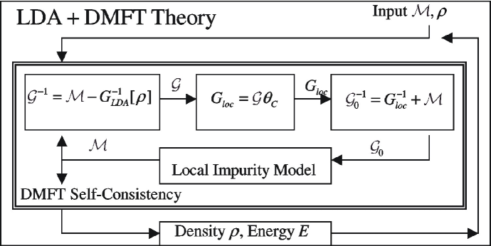
Figure 4: Illustration of self-consistent cycle in spectral density functional theory with LDA+DMFT approximation: double iterational cycle consists of the innner DMFT loop and outer (density plus total energy) loop.

Iterations over the density are not complicated to incorporate in the programs for electronic structure calculations. The spherical part of the density at a given site can be written approximately using the atomic sphere approximation as an integral over the partial density of states $N_{l}(E)$ till the Fermi level $E_{F}$

$$\rho(r)=\sum_{l}\int_{-\infty}^{E_{F}}N_{l}(E)\varphi_{l}^{2}(r,E)dE$$ (60)

where $\varphi_{l}(r,E)$ are the solutions of the radial Schrödinger equation. Usually these are constructed using spherical part of the LDA potential but in the present context the non–local self–energy operator needs to be utilizedZeinLGW :

$$(-\nabla_{rl}^{2}-E)\varphi_{l}(r,E)+\int\mathcal{M}_{eff}(r,r^{\prime},E)\varphi_{l}(r^{\prime},E)r^{2}dr=0$$ (61)

Expression (60) can be simplified further if we assume a Taylor expansion of $\varphi_{l}(r,E)$=$\varphi_{l}(r,E_{\nu l})+(E-E_{\nu l})\dot{\varphi}_{l}(r,E_{\nu l})$ around some linearization energies $E_{\nu l}$ taken at the centers of gravities of the occupied energy bands, i.e. $E_{\nu l}=\int_{-\infty}^{E_{F}}EN_{l}(E)dE/\int_{-\infty}^{E_{F}}N_{l}(E)dE$. During the iterations, DMFT modifies the density of states, $\Delta N_{l}(E),$ which leads to the change $\Delta\rho(r)$ of the density. The latter has a feedback onto the change $\Delta\varphi_{l}(r,E)$ [or changes $\Delta\varphi_{l}(r,E_{\nu l}),\Delta\dot{\varphi}_{l}(r,E_{\nu l})$]. If we assume that these changes are small comparing to the original LDA values, we can work out a linear response relationship for the density

$$\Delta\rho(r)=\sum_{l}\int_{-\infty}^{E_{F}}\Delta N_{l}(E)\varphi_{l}^{2}(r,E)dE+\sum_{l}\int_{-\infty}^{E_{F}}N_{l}(E)\varphi_{l}(r,E)\Delta\varphi_{l}(r,E)dE+\sum_{l}N_{l}(E_{F})\varphi_{l}^{2}(r,E_{F})\Delta E_{F}$$ (62)

and for the LDA potential

$$\Delta V_{LDA}(r)=e^{2}\int\frac{\Delta\rho(r^{\prime})}{|\mathbf{r}-\mathbf{r}^{\prime}|}d\mathbf{r}^{\prime}+\frac{dV_{xc}^{LDA}}{d\rho}\Delta\rho(r)$$ (63)

Thus, to first order, these are the quantities which are iterated in the external density loop of the spectral density functional as shown on Fig. 4.

The main physical point of the LDA+DMFT methodology is identification of a subset of the correlated orbitals $\{\chi_{a}\}$ which is separated from the full Hilbert space $\{\chi_{\alpha}\}.$ In the case like Pu, this is the subset of f–electron orbitals. In other situations, this subset can be isolated based on physical grounds. If $\{\chi_{a}\}$ is appropriately constructed Wannier representation, this subset may describe the bands crossing the Fermi level. We expect the dynamical self–energy corrections to appear at first place only within the subset $\{\chi_{a}\}$. However, changes in the electronic densities of states, $\Delta N_{l}(E),$ will appear for all light and heavy electrons.

We did not discuss so far the relaxation of the screened Coulomb interaction $\mathcal{W}(\mathbf{r},\mathbf{r}^{\prime},i\omega)$, which, in principle, needs to be done during the self–consistency in parallel to $\mathcal{G}(\mathbf{r},\mathbf{r}^{\prime},i\omega)$. We stress that the short–range behavior appears only for the local effective susceptibility $\mathcal{P}(\mathbf{r},\mathbf{r}^{\prime},i\omega)$ in (33) and means its fast decay when $\mathbf{r}$ departs from $\mathbf{r}^{\prime}.$ Contrary, the function $\mathcal{W}(\mathbf{r},\mathbf{r}^{\prime},i\omega)$ can be as long range as the bare Coulomb interaction if necessary. This is dictated by Eq. (33) and is similar to the relationship (20) between $\mathcal{G}$ and $\mathcal{M}_{int}.$

The locality  assumption for $\mathcal{P}$ should simplify the self–consistency over $\mathcal{W}$. This should be faster than the one employed in the full GW method which formally tries to compute full $\Pi(\mathbf{r},\mathbf{r}^{\prime},i\omega).$ In the language of local orbital representation $\{\chi_{\alpha}\},$ this means computation of all matrix elements for $\Pi_{\alpha\beta}(\mathbf{R}-\mathbf{R}^{\prime},i\omega)$ or its Fourier transform $\Pi_{\alpha\beta}(\mathbf{k},i\omega)$ as compared to the site–diagonal ($\delta_{RR^{\prime}})$ or small cluster cases of SDFT. This will be discussed below in connection to the recently proposed Zein ; ReviewTsvelik local version of the GW method.

So far we did not mention the problem of the optimal choice of the double counting corrections. This is discussed below in connection to the LDA+U method.

II.5 Double Counting and LDA+U Method

Historically, the LDA+U method has been introduced AnisimovLDA+U as an extension of the local spin density approximation (LSDA) to treat the ordered phases of Mott insulating solids. In this respect it is a natural extension of LSDA. However, this method was first to recognize that a better energy functional can be constructed if not only the density but the density matrix of correlated orbitals is brought into the density functional. We have discussed the correlated subset $\{\chi_{a}\}$ and local Green functions $G_{loc,\alpha\beta}(i\omega)$ in connection to the LDA+DMFT method. The density matrix $n_{ab}$ is related to the correlated subblock of the local Green function

$$n_{ab}=T\sum_{i\omega}e^{i\omega 0^{+}}G_{loc,ab}(i\omega)$$ (64)

Therefore, the LDA+U method can be viewed as an approximation (Hartree–Fock approximation) to the spectral density functional within LDA+DMFT.

The correct interaction energy among the correlated electrons can be written down explicitly using the Hartree–Fock approximation. In our language the LDA+DMFT interaction energy functional (55) is rewritten in the form

$$\Phi_{LDA+U}[\rho,n_{ab}]=E_{H}[\rho]+\Phi_{xc}^{LDA}[\rho]+\tilde{\Phi}_{U}[n_{ab}]-\Phi_{DC}[\bar{n}_{c}]$$ (65)

where the functional form $\tilde{\Phi}_{U}[n_{ab}]$ is known explicitly:

$$\tilde{\Phi}_{U}[n_{ab}]=\frac{1}{2}\sum_{abcd}(U_{acbd}-U_{acdb})n_{ab}n_{cd}$$ (66)

Here, indexes $a,b,c,d$ involve fixed angular momentum $l$ of the heavy orbitals and run over magnetic $m$ and spin $\sigma$ quantum numbers. The on–site Coulomb interaction matrix $U_{abcd}$ is the on–site Coulomb interaction matrix element $V_{\alpha=a\beta=b\gamma=c\delta=d}^{RRRR}$ appeared in (54) which is again taken for the subblock of the heavy orbitals. Note that sometimes $U_{abcd}$ is defined as $V_{\alpha=a\beta=c\gamma=b\delta=d}^{RRRR}.$

The double counting term $\Phi_{DC}[n_{ab}]$ needs to be introduced since both the L(S)DA and U terms account for the same interaction energy between the correlated orbitals. This includes in first place the Hartree part. However, the precise form of the double counting is unclear due to non–linear nature of the LDA exchange–correlation energy. In practice, it was proposedReviewLDA+U that the form for $\Phi_{DC}$ is

$$\Phi_{DC}[\bar{n}_{c}]=\frac{1}{2}\bar{U}\bar{n}_{c}(\bar{n}_{c}-1)-\frac{1}{2}\bar{J}[\bar{n}_{c}^{\uparrow}(\bar{n}_{c}^{\uparrow}-1)+\bar{n}_{c}^{\downarrow}(\bar{n}_{c}^{\downarrow}-1)].$$ (67)

where $\bar{U}=\frac{1}{(2l+1)^{2}}\sum_{ab}U_{abab}$ , $\bar{J}=\bar{U}-\frac{1}{2l(2l+1)}\sum_{ab}(U_{abab}-U_{abba})$and where $\bar{n}_{c}^{\sigma}=\sum_{a\in l_{c}}n_{aa}\delta_{\sigma_{a}\sigma},$ $\bar{n}_{c}=\bar{n}_{c}^{\uparrow}+\bar{n}_{c}^{\downarrow}.$ Some other forms of the double countings have also been discussed in Ref. Mazin, .

The minimization of the functional $\Gamma_{LDA+U}[\rho,n_{ab}]$ is now performed. The self–energy correction in (58) appears as the orbital dependent correction $\mathcal{\tilde{M}}_{ab}-V_{ab}^{DC}$:

$$\mathcal{\tilde{M}}_{ab} = \frac{\delta\tilde{\Phi}_{U}}{\delta n_{ab}}=\sum_{cd}(U_{acbd}-U_{acdb})n_{cd}$$ (68)

$$V_{ab}^{DC} = \frac{\delta\Phi_{DC}}{\delta n_{ab}}=\delta_{ab}[\bar{U}(\bar{n}_{c}-\frac{1}{2})-\bar{J}(\bar{n}_{c}^{\sigma}-\frac{1}{2})]$$ (69)

While the correction is static, it is best viewed as the Hartree–Fock approximation to the self–energy $\mathcal{M}_{ab}(i\omega)$ within the LDA+DMFT method. Note that such interpretation allows us to utilize double counting forms within LDA+DMFT as $\mathcal{\tilde{M}}(\mathbf{r},\mathbf{r}^{\prime},i\infty)$ or $\mathcal{\tilde{M}}(\mathbf{r},\mathbf{r}^{\prime},i0)$. Note also that the solution of the impurity problem collapses in the LDA+U method since the self–energy is known analytically by formula (68).

From a practical point of view, despite the great success of the LDA+U theory in predicting materials properties of correlated solids ReviewLDA+U there are obvious problems with this approach when applied to metals or to systems where the orbital symmetries are not broken. They stem from the well–known deficiencies of the Hartree–Fock approximation. The most noticeable is that it only describes spectra of magnetically ordered systems which have Hubbard bands. We have however argued that a correct treatment of the electronic structure of strongly correlated systems has to treat both Hubbard bands and quasiparticle bands on the same footing. Another problem occurs in the paramagnetic phase of Mott insulators: in the absence of any broken symmetry the LDA+U method reduces to the LDA, and the gap collapses. In systems like NiO where the gap is of the order of eV, but the Neel temperature is a few hundred Kelvin, it is unphysical to assume that the gap and the magnetic ordering are related. For this reason the LDA+U predicts magnetic order in cases that it is not observed, as, e.g., in the case of Pu PuPRL .

II.6 Local GW Approximation

We now discuss the relaxation of the screened Coulomb interaction $\mathcal{W}(\mathbf{r},\mathbf{r}^{\prime},i\omega)$ which appeared in the spectral density functional formulation of the problem. Both LDA+DMFT and LDA+U methods parametrize the interaction $\mathcal{W}$ with optimally screened set of parameters, such, e.g, as the matrix $U_{abcd}$ appeared in (66). This matrix is supposed to be given by an external calculation such, e.g., as the constrained LDA method ConstrainedDFT . To determine this interaction self consistently an additional self–consistency loop described by the equations (33) and (46) has to be switched on together with calculation of the local susceptibility $\mathcal{P}(\mathbf{r},\mathbf{r}^{\prime},i\omega)$ by the impurity solver. This brings a truly self–consistent ab initio method without input parameters and the double counting problems.

A simplified version of this method has been recently proposed ReviewTsvelik ; Zein which is known as a local version of the GW method (LGW). Within the spectral density functional theory, this approximation appears as approximation to the functional $\Psi_{SDF}[G_{loc},W_{loc}]$ taken in the form

$$\Psi_{LGW}[G_{loc},W_{loc}]=-\frac{1}{2}\mathrm{Tr}G_{loc}W_{loc}G_{loc}$$ (70)

As a result, the susceptibility $\mathcal{P}(\mathbf{r},\mathbf{r}^{\prime},i\omega)$ is approximated by the product of two local Green functions, i.e.$\mathcal{P}=-2\delta\Psi_{LGW}/\delta W_{loc}=G_{loc}G_{loc},$ and the exchange–correlation part of our mass operator is approximated by the local GW diagram, i.e. $\mathcal{M}_{xc}=\delta\Psi_{LGW}/\delta G_{loc}=-G_{loc}W_{loc}$.

Thus, the impurity model is solved and the procedure can be made self–consistent: For a given $\mathcal{M}_{int}$ and $\mathcal{P}$, the Dyson equations (20), (37) for $\mathcal{G}$ and $\mathcal{W}$ are solved. Then, the local quantities $G_{loc,}$ $W_{loc}$ are generated and used to find new $\mathcal{M}_{int}$ and $\mathcal{P}$ thus avoiding the computation of the bath Green function $\mathcal{G}_{0}$ after (45), and the interaction $\mathcal{V}$, after (46).

Note that since the local GW approximation (70) is relatively cheap from computational point of view, its implementation on a cluster and for all orbitals should not be a problem. The results of the single–site approximation for the local quantities have been developed independently and reported in the literature.Zein . The cluster extension is currently being performed and the results will be reported elsewhere ZeinLGW .

Note finally that the local GW approximation is not the only one which can be implemented as the simplified impurity solver. For example, another popular approximation known as the fluctuational exchange approximation (FLEX) can be worked out along the same lines. Note also that the combination of the DMFT and full GW diagram has been recently proposed ReviewTsvelik ; Georges and a simplified implementation for Ni Georges , and for a model Hamiltonian Ping have been carried out. This procedure incorporates full k–dependence of the self–energy known diagrammatically within GW together with the additional local DMFT diagrams.

III Calculation of Local Green Function

The solution of the Dyson equations described in the previous section for a given strongly correlated material requires the calculation of the local Green function during the iterations towards self–consistency. This is very similar to the procedure in the density functional theory, when the charge density is computed. A big advantage of DFT is the use of Kohn–Sham orbitals which reduces the equation (22) for the Kohn–Sham Green function to a set of one–particle Schrödinger’s like equations for the wave functions. As a result the kinetic energy contribution is calculated directly and the evaluation of the total energy of a solid is not a problem. Here, a similar algorithm will be described for the energy–dependent Dyson equation, the solution in terms of the linear–muffin–tin orbital basis set will be discussed, and the formula for evaluating the total energy will be given.

III.1 Energy Resolved One-Particle Representation

We introduced the auxiliary Green function $\mathcal{G}(\mathbf{r},\mathbf{r}^{\prime},i\omega)$ to deal with the kinetic part of the action in SDFT. It satisfies to the Dyson equation (9). Let us now introduce the representation of generalized energy–dependent one-particle states

$$\mathcal{G}(\mathbf{r},\mathbf{r}^{\prime},i\omega) = \sum_{\mathbf{k}j}\frac{\psi_{\mathbf{k}j\omega}^{R}(\mathbf{r})\psi_{\mathbf{k}j\omega}^{L}(\mathbf{r}^{\prime})}{i\omega+\mu-E_{\mathbf{k}j\omega}}$$ (71)

$$\mathcal{G}^{-1}(\mathbf{r},\mathbf{r}^{\prime},i\omega) = \sum_{\mathbf{k}j}\psi_{\mathbf{k}j\omega}^{R}(\mathbf{r})(i\omega+\mu-E_{\mathbf{k}j\omega})\psi_{\mathbf{k}j\omega}^{L}(\mathbf{r}^{\prime})$$ (72)

where the left $\psi_{\mathbf{k}j\omega}^{L}(\mathbf{r})$ and right $\psi_{\mathbf{k}j\omega}^{R}(\mathbf{r})$ states satisfy to the following Dyson equations:

$$[-\nabla^{2}+V_{ext}(\mathbf{r})+V_{H}(\mathbf{r})]\psi_{\mathbf{k}j\omega}^{R}(\mathbf{r})+\int\mathcal{M}_{xc}(\mathbf{r},\mathbf{r}^{\prime},i\omega)\psi_{\mathbf{k}j\omega}^{R}(\mathbf{r}^{\prime})d\mathbf{r}^{\prime} = E_{\mathbf{k}j\omega}\psi_{\mathbf{k}j\omega}^{R}(\mathbf{r})$$ (73)

$$[-\nabla^{2}+V_{ext}(\mathbf{r}^{\prime})+V_{H}(\mathbf{r}^{\prime})]\psi_{\mathbf{k}j\omega}^{L}(\mathbf{r}^{\prime})+\int\psi_{\mathbf{k}j\omega}^{L}(\mathbf{r})\mathcal{M}_{xc}(\mathbf{r},\mathbf{r}^{\prime},i\omega)d\mathbf{r} = E_{\mathbf{k}j\omega}\psi_{\mathbf{k}j\omega}^{L}(\mathbf{r}^{\prime})$$ (74)

[we dropped the imaginary unit for simplicity in the notation $\psi_{\mathbf{k}j\omega}(\mathbf{r})$ which shall be thought as a shortened version of $\psi_{\mathbf{k}j}(\mathbf{r},i\omega)$]. These equations should be considered as the eigenvalue problems with complex non-hermitian self–energy. As a result, the eigenvalues $E_{\mathbf{k}j\omega}$ [a shortened form for $E_{\mathbf{k}j}(i\omega)$] being the same for both equations are complex in general. The explicit dependency on the frequency $i\omega$ in both eigenvectors and eigenvalues comes from the self–energy. Note that left and right eigenfunctions are orthonormal

$$\int d\mathbf{r}\psi_{\mathbf{k}j\omega}^{L}(\mathbf{r})\psi_{\mathbf{k}j^{\prime}\omega}^{R}(\mathbf{r})\mathbf{=}\delta_{jj^{\prime}}$$ (75)

and can be used to evaluate the charge density of a given system using the Matsubara sum and the integral over the k–space:

$$\rho(\mathbf{r})=T\sum_{i\omega}\sum_{\mathbf{k}j}g_{\mathbf{k}j\omega}\psi_{\mathbf{k}j\omega}^{L}(\mathbf{r})\psi_{\mathbf{k}j\omega}^{R}(\mathbf{r})e^{i\omega 0^{+}}$$ (76)

where

$$g_{\mathbf{k}j\omega}=\frac{1}{i\omega+\mu-E_{\mathbf{k}j\omega}}$$ (77)

We  have cast the notation of spectral density theory in a form similar to DFT. The function $g_{\mathbf{k}j\omega}$ is the Green function in the orthogonal left/right representation which plays a role of a ”frequency dependent occupation number”.

It needs to be pointed out that the frequency dependent energy bands $E_{\mathbf{k}j\omega}$ represent an auxiliary set of complex eigenvalues. These are not the true poles of the exact one–electron Green function $G(\mathbf{r},\mathbf{r}^{\prime},z)$ considered at complex z plane. However, they are designed to reproduce the local spectral density of the system. Note also that these bands $E_{\mathbf{k}jz}$ are not the true poles of the auxiliary Green function $\mathcal{G}(\mathbf{r},\mathbf{r}^{\prime},z).$ The latter ones still need to be located by solving a non–linear equation corresponding to the singularities in the expression (71) after analytic continuation to real frequency. For a one–band case this equation is simply: $z+\mu-E_{\mathbf{k}z}=0$ , whose solution delivers the quasiparticle dispersion $Z_{\mathbf{k}}$. General knowledge of the poles positions $Z_{\mathbf{k}j}$ will allow us to write an alternative expression for $\mathcal{G}$ which is similar to (71), but with the eigenvectors found at $Z_{\mathbf{k}j}$ thus carrying out no auxiliary frequency dependence. These poles are the real one–electron excitational spectra in case $\mathcal{G}$ is a good approximation to $G$. However, the use of (71) is advantageous, since it avoids additional search of poles and allows direct evaluation of the local spectral and charge densities the system.

The energy–dependent representation allows us to obtain a very compact expression for the total energy. As we have argued, the entropy terms are more difficult to evaluate. However, they are generally small as long as we stay at low temperatures. The pure kinetic part of the free energy expressed via [see, Eq.(39)]

$$Tr\ln\mathcal{G}-Tr\mathcal{M}_{eff}\mathcal{G}=T\sum_{i\omega}e^{i\omega 0^{+}}\int d\mathbf{r}d\mathbf{r}^{\prime}\ln\mathcal{G}(\mathbf{r},\mathbf{r}^{\prime},i\omega)-T\sum_{i\omega}\int d\mathbf{r}d\mathbf{r}^{\prime}\mathcal{M}_{eff}(\mathbf{r},\mathbf{r}^{\prime},i\omega)\mathcal{G}(\mathbf{r}^{\prime},\mathbf{r},i\omega)$$ (78)

needs to be separated onto the energy and entropy terms. Both contributions can be evaluated without a problem, but in light of neglecting the entropy correction in the interaction part, we concentrate on evaluating  the kinetic energy only:

$$T\sum_{i\omega}e^{i\omega 0^{+}}\int d\mathbf{r}\left[(-\nabla_{\mathbf{r}}^{2})\mathcal{G}(\mathbf{r},\mathbf{r}^{\prime},i\omega)\right]_{\mathbf{r}=\mathbf{r}^{\prime}}=T\sum_{i\omega}e^{i\omega 0^{+}}\sum_{\mathbf{k}j}\frac{\langle\psi_{\mathbf{k}j\omega}^{L}|-\nabla^{2}|\psi_{\mathbf{k}j\omega}^{R}\rangle}{i\omega+\mu-E_{\mathbf{k}j\omega}}$$ (79)

The SDFT total energy formula is now arrived by utilizing the relationship $E_{\mathbf{k}j\omega}=\langle\psi_{\mathbf{k}j\omega}^{L}|-\nabla^{2}+\mathcal{M}_{eff}|\psi_{\mathbf{k}j\omega}^{R}\rangle=\langle\psi_{\mathbf{k}j\omega}^{L}|-\nabla^{2}+V_{ext}+V_{H}+\mathcal{M}_{xc}|\psi_{\mathbf{k}j\omega}^{R}\rangle$:

$$E_{SDF}=T\sum_{i\omega}e^{i\omega 0^{+}}\sum_{\mathbf{k}j}g_{\mathbf{k}j\omega}E_{\mathbf{k}j\omega}-T\sum_{i\omega}\int d\mathbf{r}d\mathbf{r}^{\prime}\mathcal{M}_{eff}(\mathbf{r,r}^{\prime},i\omega)\mathcal{G}(\mathbf{r}^{\prime},\mathbf{r},i\omega)+$$

$$+\int d\mathbf{r}V_{ext}(\mathbf{r})\rho(\mathbf{r})+\frac{1}{2}\int d\mathbf{r}V_{H}(\mathbf{r})\rho(\mathbf{r})+\frac{1}{2}T\sum_{i\omega}\int d\mathbf{r}d\mathbf{r}^{\prime}\mathcal{M}_{xc}(\mathbf{r,r}^{\prime},i\omega)G_{loc}(\mathbf{r}^{\prime},\mathbf{r},i\omega)$$ (80)

If the self–energy is considered as input to the iteration while the Green function is the output, near stationary point, it should have a convergency faster than the convergency in the Green function.

It is instructive to consider the non–interactive limit when the self–energy represents a local energy–independent potential, say, the ground–state Kohn Sham potential of the density functional theory. This provides an important test for our many-body calculation. It is trivial to see that in the DFT limit, we obtain the Kohn–Sham eigenfunctions

$$\psi_{\mathbf{k}j\omega}^{R}(\mathbf{r}) \rightarrow \psi_{\mathbf{k}j}(\mathbf{r})$$ (81)

$$\psi_{\mathbf{k}j\omega}^{L}(\mathbf{r}) \rightarrow \psi_{\mathbf{k}j}^{\ast}(\mathbf{r})$$ (82)

$$E_{\mathbf{k}j\omega} \rightarrow E_{\mathbf{k}j}$$ (83)

and the one–electron energy bands are no longer frequency dependent. The sum over Matsubara frequencies in the expression for the charge density (76) can be performed analytically using the expression for the Fermi–Diraq occupation numbers:

$$f_{\mathbf{k}j}=\frac{1}{e^{(E_{\mathbf{k}j}-\mu)/T}+1}=T\sum_{i\omega}\frac{e^{i\omega 0^{+}}}{i\omega+\mu-E_{\mathbf{k}j}}$$ (84)

and the formula (76) collapses to the standard expression for the density of non–interacting fermions. The total energy expression (80) is converted back to the DFT expression for the total energy since the eigenvalue $E_{\mathbf{k}j\omega}$ becomes the DFT band structure $E_{\mathbf{k}j},$ and the summation over Matsubara frequencies $T\sum_{i\omega}e^{i\omega 0^{+}}g_{\mathbf{k}j\omega}$ gives according to (84) the Fermi–Diraq occupation number $f_{\mathbf{k}j}$. The standard DFT expression is recovered:

$$E_{DFT}=\sum_{\mathbf{k}j}f_{\mathbf{k}j}E_{\mathbf{k}j}-\int d\mathbf{r}V_{eff}(\mathbf{r})\rho(\mathbf{r})+\int d\mathbf{r}V_{ext}(\mathbf{r})\rho(\mathbf{r})+\frac{1}{2}\int d\mathbf{r}V_{H}(\mathbf{r})\rho(\mathbf{r})+E_{xc}[\rho]$$ (85)

where $E_{\mathbf{k}j}=\langle\psi_{\mathbf{k}j}|-\nabla^{2}+V_{eff}|\psi_{\mathbf{k}j}\rangle=\langle\psi_{\mathbf{k}j}|-\nabla^{2}+V_{ext}+V_{H}+V_{xc}|\psi_{\mathbf{k}j}\rangle.$

III.2 Use of Linear Muffin–Tin Orbitals

The next problem is to solve the Dyson equation for the eigenvalues. The sophisticated basis sets developed to solve the one–electron Schrödinger equation can be directly used in this case. We utilize the LMTO method described extensively in the past literature OKA-LMTO ; TBLMTO ; SavrasovLMTO as it provides a minimal atom–centered local orbital basis set ideally suited for the electronic structure calculation. Within the LMTO basis, the full Green function is represented as a sum

$$\mathcal{G}(\mathbf{r},\mathbf{r}^{\prime},i\omega)=\sum_{\mathbf{k}}\sum_{\alpha\beta}\chi_{\alpha}^{\mathbf{k}}(\mathbf{r})\mathcal{G}_{\alpha\beta}(\mathbf{k},i\omega)\chi_{\beta}^{\mathbf{k\ast}}(\mathbf{r}^{\prime})$$ (86)

and, as we have argued in the previous section, the matrix $\mathcal{G}_{\alpha\beta}(\mathbf{k},i\omega)$ needs to be considered as a variable in the spectral density functional. The stationarity yields the equation for the Green function

$$\mathcal{G}_{\alpha\beta}(\mathbf{k},i\omega)=\left[(i\omega+\mu)\hat{O}(\mathbf{k})-\hat{h}^{(0)}(\mathbf{k})-\mathcal{M}_{int}(\mathbf{k},i\omega)\right]_{\alpha\beta}^{-1}$$ (87)

where the overlap matrix $O_{\alpha\beta}(\mathbf{k})=\langle\chi_{\alpha}^{\mathbf{k}}|\chi_{\beta}^{\mathbf{k}}\rangle,$ the non–interacting Hamiltonian matrix $h_{\alpha\beta}^{(0)}(\mathbf{k})=\langle\chi_{\alpha}^{\mathbf{k}}|-\nabla^{2}+V_{ext}(\mathbf{r})|\chi_{\beta}^{\mathbf{k}}\rangle$ and the self–energy formally comes as a matrix element

$$\mathcal{M}_{int,\alpha\beta}(\mathbf{k},i\omega)=\int d\mathbf{r}d\mathbf{r}^{\prime}\chi_{\alpha}^{\mathbf{k\ast}}(\mathbf{r})\mathcal{M}_{int}(\mathbf{r},\mathbf{r}^{\prime},i\omega)\chi_{\beta}^{\mathbf{k}}(\mathbf{r}^{\prime})$$ (88)

over the LMTOs. Again, it is worth to point out that the self–energy here depends on $\mathbf{k}$ via the orbitals even if the single–impurity case is considered. In calculations performed on a cluster, the self–energy will also pick its non–trivial $\mathbf{k}$–dependence coming from the nearest sites.

While formally valid, the present approach is not very efficient since the Green function $\mathcal{G}(\mathbf{r},\mathbf{r}^{\prime},i\omega)$ has to be evaluated via (86). This is the $\mathbf{k}$–integral which has poles in a complex frequency plane, and integrating singular functions need to be performed with care. In this respect, we adopt the eigenvalue representation (71). We expand the energy–dependent states in terms of the LMTO basis $\{\chi_{\alpha}^{\mathbf{k}}\}$ as follows:

$$\psi_{\mathbf{k}j\omega}^{R(L)}(\mathbf{r})=\sum_{\alpha}A_{\alpha}^{\mathbf{k}j\omega,R(L)}\chi_{\alpha}^{\mathbf{k}}(\mathbf{r})$$ (89)

The unknown coefficients $A_{\alpha}^{\mathbf{k}j\omega,R(L)}$ are now the quantities which have to be considered as variables in the spectral density functional. The stationarity yields the equations

$$\sum_{\beta}\left[h_{\alpha\beta}^{(0)}(\mathbf{k})+\mathcal{M}_{int,\alpha\beta}(\mathbf{k},i\omega)-E_{\mathbf{k}j\omega}O_{\alpha\beta}(\mathbf{k})\right]A_{\beta}^{\mathbf{k}j\omega,R} = 0$$ (90)

$$\sum_{\alpha}A_{\alpha}^{\mathbf{k}j\omega,L}\left[h_{\alpha\beta}^{(0)}(\mathbf{k})+\mathcal{M}_{int,\alpha\beta}(\mathbf{k},i\omega)-E_{\mathbf{k}j\omega}O_{\alpha\beta}(\mathbf{k})\right] = 0$$ (91)

These are the non–hermitian eigenvalue problems solved by standard numerical methods. The orthogonality condition involving the overlap matrix is

$$\sum_{\alpha\beta}A_{\alpha}^{\mathbf{k}j\omega,L}O_{\alpha\beta}(\mathbf{k})A_{\beta}^{\mathbf{k}j^{\prime}\omega,R}=\delta_{jj^{\prime}}$$ (92)

Note that the present algorithm just inverts the matrix (87) with help of the ”right” and ”left” eigenstates. The Green function (87) in the basis of its eigenvectors becomes

$$\mathcal{G}_{\alpha\beta}(\mathbf{k},i\omega)=\sum_{j}\frac{A_{\alpha}^{\mathbf{k}j\omega,R}A_{\beta}^{\mathbf{k}j\omega,L}}{i\omega+\mu-E_{\mathbf{k}j\omega}}$$ (93)

This formula can be safely used to compute the Green function as the integral over the Brillouin zone, Eq. (86), because the energy denominator can be integrated analytically using the tetrahedron method Wigneron .

Our next topic here is the evaluation of the bath Green function $\mathcal{G}_{0}(\mathbf{r},\mathbf{r}^{\prime},i\omega)$. It can be found from the integral equation

$$\mathcal{G}_{0}(\mathbf{r},\mathbf{r}^{\prime},i\omega)=G_{loc}(\mathbf{r},\mathbf{r}^{\prime},i\omega)-\int d\mathbf{r}^{\prime\prime}d\mathbf{r}^{\prime\prime\prime}G_{loc}(\mathbf{r},\mathbf{r}^{\prime\prime},i\omega)\mathcal{M}_{int}(\mathbf{r}^{\prime\prime},\mathbf{r}^{\prime\prime\prime},i\omega)\mathcal{G}_{0}(\mathbf{r}^{\prime\prime\prime},\mathbf{r},i\omega)$$ (94)

where $\mathbf{r}$ and $\mathbf{r}^{\prime}$ run over $\Omega_{loc}$ In order to solve this equation, it is useful to represent $\mathbf{r}=\mathbf{\rho}+\mathbf{R,}$ $\mathbf{r}^{\prime}=\mathbf{\rho}^{\prime}+\mathbf{R}^{\prime}\mathbf{,}$ and redenote $\mathcal{G}_{0}(\mathbf{r},\mathbf{r}^{\prime},i\omega)=\mathcal{G}_{0,RR^{\prime}}(\mathbf{\rho},\mathbf{\rho}^{\prime},i\omega),G_{loc}(\mathbf{r},\mathbf{r}^{\prime},i\omega)=G_{loc,RR^{\prime}}(\mathbf{\rho},\mathbf{\rho}^{\prime},i\omega),\mathcal{M}_{int}(\mathbf{r},\mathbf{r}^{\prime},i\omega)=\mathcal{M}_{int,RR^{\prime}}(\mathbf{\rho},\mathbf{\rho}^{\prime},i\omega).$ Considering one atom per unit cell let us see how this can be solved using single–kappa LMTO–ASA method. The generalization to multiatomic systems with multiple kappa basis sets as well as inclusion of full potential terms in the calculation can be done along the same lines. The form of the LMTO basis function inside the sphere centered at $\mathbf{R}$ is

$$\chi_{\alpha}^{\mathbf{k}}(\mathbf{r})=\chi_{\alpha}^{\mathbf{k}}(\mathbf{\rho})e^{i\mathbf{kR}}=e^{i\mathbf{kR}}[\Phi_{\alpha}^{H}(\mathbf{\rho})+\sum_{L}\Phi_{L}^{J}(\mathbf{\rho})S_{L\alpha}^{\mathbf{k}}]$$ (95)

where $S_{L\alpha}^{\mathbf{k}}$ are the structure constants of the LMTO  method and where $\Phi_{L}^{H,J}(\mathbf{\rho})$ are linear combinations of the solutions of the radial Schrödinger equation taken at spherical part of the potential and matched to the spherical Hankel (H) and Bessel (J) functions at the muffin–tin sphere boundary as well as their energy derivatives taken at some set of energies $E_{\nu l}$ at the center of interest. The local Green function can be represented in this basis set as follows

$$G_{loc,RR^{\prime}}(\mathbf{\rho},\mathbf{\rho}^{\prime},i\omega)=\sum_{LL^{\prime}}\sum_{\mu,\nu=H,J}\Phi_{L}^{(\mu)}(\mathbf{\rho})G_{loc,LRL^{\prime}R^{\prime}}^{(\mu\nu)}(i\omega)\Phi_{L^{\prime}}^{(\nu)\ast}(\mathbf{\rho}^{\prime})$$ (96)

where the matrices $G_{loc,\alpha R\beta R^{\prime}}^{HH}(i\omega),G_{loc,\alpha RL^{\prime}R^{\prime}}^{HJ}(i\omega),G_{loc,LR\beta R^{\prime}}^{JH}(i\omega),G_{loc,LRL^{\prime}R^{\prime}}^{JJ}(i\omega)$ (indexes $R$ and $R^{\prime}$ are restricted to a cluster) are given by the following Brillouin zone integrals

$$G_{loc,LRL^{\prime}R^{\prime}}^{(\mu\nu)}(i\omega)=\sum_{\mathbf{k}j}\frac{A_{L(\mu)}^{\mathbf{k}j\omega,R}A_{L^{\prime}(\nu)}^{\mathbf{k}j\omega,L}}{i\omega+\mu-E_{\mathbf{k}j\omega}}e^{i\mathbf{k}(\mathbf{R}-\mathbf{R}^{\prime})}$$ (97)

Here $A_{L(H)}^{\mathbf{k}j\omega,R(L)}$ are the original eigenvectors $A_{L}^{\mathbf{k}j\omega,R(L)}$ and $A_{L(J)}^{\mathbf{k}j\omega,L}=\sum_{\alpha}A_{\alpha}^{\mathbf{k}j\omega,L}S_{L\alpha}^{\mathbf{k}},$ $A_{L(J)}^{\mathbf{k}j\omega,R}=\sum_{\alpha}S_{L\alpha}^{\mathbf{k\ast}}A_{\alpha}^{\mathbf{k}j\omega,R}$ are the convolutions of the eigenvectors with the LMTO structure constants. We now utilize a similar representation for the bath Green function

$$\mathcal{G}_{0,RR^{\prime}}(\mathbf{\rho},\mathbf{\rho}^{\prime},i\omega)=\sum_{LL^{\prime}}\sum_{\mu,\nu=H,J}\Phi_{L}^{(\mu)}(\mathbf{\rho})\mathcal{G}_{0,LRL^{\prime}R^{\prime}}^{(\mu\nu)}(i\omega)\Phi_{L^{\prime}}^{(\nu)\ast}(\mathbf{\rho}^{\prime})$$ (98)

where the matrices $\mathcal{G}_{0,\alpha R\beta R^{\prime}}^{HH}(i\omega),\mathcal{G}_{0,\alpha RL^{\prime}R^{\prime}}^{HJ}(i\omega),\mathcal{G}_{0,LR\beta R^{\prime}}^{JH}(i\omega),\mathcal{G}_{0,LRL^{\prime}R^{\prime}}^{JJ}(i\omega)$ can be found from the following  Dyson equation (where the matrices sizes have been enlarged by a factor of 2)

$$\mathcal{G}_{0,LRL^{\prime}R^{\prime}}^{(\mu\nu)-1}(i\omega)=G_{loc,LRL^{\prime}R^{\prime}}^{(\mu\nu)-1}(i\omega)+\mathcal{M}_{int,LRL^{\prime}R^{\prime}}^{(\mu\nu)}(i\omega)$$ (99)

with the self–energy matrices are defined as follows

$$\mathcal{M}_{int,LRL^{\prime}R^{\prime}}^{(\mu\nu)}(i\omega)=\int d\mathbf{\rho}d\mathbf{\rho}^{\prime}\Phi_{L}^{(\mu)\ast}(\mathbf{\rho})\mathcal{M}_{int,RR^{\prime}}(\mathbf{\rho},\mathbf{\rho}^{\prime},i\omega)\Phi_{L^{\prime}}^{(\nu)}(\mathbf{\rho}^{\prime})$$ (100)

The solution of the impurity model with $\mathcal{G}_{0,LRL^{\prime}R^{\prime}}^{(\mu\nu)}(i\omega)$ delivers new matrix elements (100). The k–dependent self–energy (88) to be used in constructing the new Green function in (87) is found first by restoring the $\mathbf{k}$–dependence from the cluster $\mathcal{M}_{int,LL^{\prime}}^{(\mu\nu)}(\mathbf{k},i\omega)=\sum_{R-R^{\prime}}\mathcal{M}_{int,LRL^{\prime}R^{\prime}}^{(\mu\nu)}(i\omega)e^{i\mathbf{k}(\mathbf{R}-\mathbf{R}^{\prime})}$ and second, restoring the $\mathbf{k}$–dependence of the LMTO basis as follows

$$\mathcal{M}_{int,\alpha\beta}(\mathbf{k},i\omega)=\mathcal{M}_{int,\alpha\beta}^{HH}(\mathbf{k},i\omega)+\sum_{L}\mathcal{M}_{int,\alpha L}^{HJ}(\mathbf{k},i\omega)S_{L\beta}^{\mathbf{k}}+\sum_{L^{\prime}}S_{L^{\prime}\alpha}^{\mathbf{k\ast}}\mathcal{M}_{int,L^{\prime}\beta}^{JH}(\mathbf{k},i\omega)+\sum_{LL^{\prime}}S_{L\alpha}^{\mathbf{k\ast}}\mathcal{M}_{int,LL^{\prime}}^{JJ}(\mathbf{k},i\omega)S_{L^{\prime}\beta}^{\mathbf{k}}$$ (101)

In practical calculations performed with the LDA+DMFT method for Pu, only the subset of orbitals $\{\chi_{a}\}$ is treated as correlated (f electrons of Pu) and a single–impurity case is considered. It is useful to separate the Hartree and LDA exchange–correlations terms. Instead of dealing with the non–interacting Hamiltonian in (87), we can rearrange the contributions to arrive

$$\mathcal{G}_{\alpha\beta}(\mathbf{k},i\omega)=\left[(i\omega+\mu)\hat{O}(\mathbf{k})-\hat{h}^{LDA}(\mathbf{k})-\Delta\mathcal{\hat{M}}(\mathbf{k},i\omega)\right]_{\alpha\beta}^{-1}$$ (102)

where $h_{\alpha\beta}^{LDA}(\mathbf{k})=\langle\chi_{\alpha}^{\mathbf{k}}|-\nabla^{2}+V_{LDA}(\mathbf{r})|\chi_{\beta}^{\mathbf{k}}\rangle$ with $V_{LDA}(\mathbf{r})=V_{ext}(\mathbf{r})+V_{H}(\mathbf{r})+V_{xc}^{LDA}(\mathbf{r}).$ The matrix $\Delta\mathcal{M}_{\alpha\beta}(\mathbf{k},i\omega)=\mathcal{\tilde{M}}_{\alpha\beta}(\mathbf{k},i\omega)-V_{\alpha\beta}^{DC}(\mathbf{k}),$ where $\mathcal{M}_{\alpha\beta}(\mathbf{k},i\omega)=\delta_{\alpha a}\delta_{\beta b}\mathcal{\tilde{M}}_{ab}(\mathbf{k},i\omega)$ and $V_{\alpha\beta}^{DC}(\mathbf{k})=\delta_{\alpha a}\delta_{\beta b}V_{ab}^{DC}(\mathbf{k})$ represent the DMFT correction and double counting term described by (69). These matrices are non–zero within the correlated subset. To accelerate the calculation of the impurity model, we can parametrize the self–energy matrix as $\mathcal{\tilde{M}}_{ab}^{(\mu\nu)}(i\omega)=\mathcal{\tilde{M}}_{ab}^{(p)}(i\omega)\langle\Phi_{a}^{(\mu)}|\Phi_{b}^{(\nu)}\rangle.$ With such parametrization, the local Green function which enters the Dyson equation should be defined as follows $G_{loc,ab}(i\omega)=\sum_{\mathbf{k}j}\sum_{\mu\nu}A_{a(\mu)}^{\mathbf{k}j\omega,R}$ $\langle\Phi_{a}^{(\mu)}|\Phi_{b}^{(\nu)}\rangle A_{b(\nu)}^{\mathbf{k}j\omega,L}/$ $(i\omega+\mu-E_{\mathbf{k}j\omega})$. This represents the generalization of a partial–density–of–state formula of the LMTO method. The bath Green function can be found from the equation: $\mathcal{G}_{0,ab}(i\omega)^{-1}=G_{loc,ab}(i\omega)^{-1}+\mathcal{\tilde{M}}_{ab}^{(p)}(i\omega)$ and can be passed to the impurity solver. The latter delivers a new self–energy $\mathcal{\tilde{M}}_{ab}^{(p)}(i\omega)$ which is then multiplied by $\langle\Phi_{a}^{(\mu)}|\Phi_{b}^{(\nu)}\rangle$ and used to reconstruct new $\mathbf{k}$–dependent self–energy after (101). Such procedure preserves all $\mathbf{k}$–dependent information coming from the orbitals.

IV Applications to Plutonium

This section describes the application of the theory to Plutonium. Pu is known to be an anomalous metal PuBook . It has six crystallographic structures. Starting from the low temperature $\alpha$ phase (0 to 100 C) with 16 atoms per unit cell it shows a series of phase transitions and ends up in relatively simple fcc $\delta$ (300–450 C) and bcc $\varepsilon$ phases (500–650 C) just before it melts. The temperature dependence of atomic volume in Pu is anomalous PuVol . It shows an enormous volume expansion between $\alpha$ and $\delta$ phases which is about 25%. Within the $\delta$ phase, the metal shows negative thermal expansion. Transition between $\delta$ and higher–temperature $\varepsilon$ phase occurs with a 5% volume collapse. Also, Pu shows anomalous resistivity behavior PuRHO characteristic for the heavy fermion systems, but neither of its phases is magnetic. The susceptibility is small and relatively temperature independent. The photoemission PuExp1 shows a strong narrow Kondo–like peak at the Fermi level consistent with large values of the linear specific heat coefficient.

Density functional based LDA and GGA calculations describe the properties of Pu incorrectly. They predict magnetic ordering PuMag . They underestimate PuLDA equilibrium volume of the $\delta$ and $\varepsilon$ phase by as much as 30% , the largest discrepancy known in LDA, which usually predicts the volume of solids within a few % accuracy even for such correlated systems as high temperature superconductors. Despite this, the volume of the $\alpha$ phase is predicted correctly by LDA PuLDA . Since the transport and thermodynamic properties of $\alpha$ and $\delta$ Pu are very similar, the nature of the $\alpha$ phase and the reason why LDA predicts accurately its structure and volume is by itself is another puzzle.

To address these questions several approaches have been developed. The LDA+U method was applied to $\delta$ Pu PuPRL ; PuLDA+U . It is able to produce the correct volume of the $\delta$ phase for values of the parameter $U\char 126\relax$4 eV consistent with atomic spectral data and constrained density functional calculations. Similar calculation has been performed by a so–called orbitally ordered density functional method PuLDA+J . However, both methods predict Pu to be magnetic, which is not observed experimentally. The LDA+U method is unable to predict the correct excitation spectrum. Also, to recover the $\alpha$ phase within LDA+U  the parameter U has to be set to zero which is inconsistent with its transport properties and with microscopic calculations of this parameter. Another approach proposed PuCore in the past is the constrained LDA approach in which some of the 5f electrons, are treated as core, while the remaining are allowed to participate in band formation. Results of the self–interaction–corrected LDA calculations have been reported PuSIC , as well as qualitative discussion of the bonding nature across the actinides series has been given Harrison .

Thus, the problem of Pu is challenging because its f-electrons are close to the Mott transition Johansson . It provides us a crucial test for our quantitative theory of strong correlations. A short version of this work has appeared already PuNature . Our implementation is based on the self–consistent LDA+DMFT method and uses the LMTO method in its tight-binding representation TBLMTO . Spin–orbit coupling effects are important for actinide compounds and have been included in the calculation for Pu. The “full potential” terms have been neglected in the calculation through the use of the atomic sphere approximation with a one-kappa LMTO basis set. The necessary $\mathbf{k}$-space integrals for evaluating Green functions and charge densities have been carried out using the tetrahedron method using (8,8,8) grid in the Brillouin zone.

We study in detail the total energy as a function of the parameter $U$ and give our predictions for the volumes in $\alpha,$ $\delta,$ and $\varepsilon$ phases. A comparative analysis of the one–electron spectra in both $\alpha$ and $\delta$ phases is also given and the comparison with the photoemission experiment PuExp1 is made. Since the dynamical mean field theory requires the solution of the Anderson impurity model for the multi-orbital f–shell of Pu, we have developed a method which, inspired by the success of the iterative perturbation theory ReviewDMFT , interpolates the self–energy between small and large frequencies. At low frequencies, the exact value of the self-energy and its slope is extracted from the Friedel sum rule and from a slave-boson treatmentGutz ; Ruck ; Fleszar . This approach is accurate as it has been shown recently to give the exact critical value of $U$ in the large degeneracy limit Parcollet  At high frequencies the self-energy behavior can be computed based on high–frequency moments expansionsHubbard1 ; Moments . The result of interpolation can be encoded into a simple form for the self–energy like the following continuous fraction expansion

$$\Sigma(i\omega)=\Sigma(i\infty)+\frac{A}{i\omega-\frac{B}{i\omega-C}}$$ (103)

where the unknown coefficients are determined to satisfy known conditions in the low– and high–frequency limits. This kind of self–energy fits Quantum Monte Carlo (QMC) data in large region of parameters, such as $U$ and doping, and where this comparison is at all possible (small degeneracy and high temperature). Thus, our approach interpolates between four major limits: small and large i$\omega$’s valid for any $U$ as well as small and large $U^{\prime}s$ (band vs. atom) valid for any $i\omega$. The analytical continuation to the real frequency axis is not a problem with the present method and avoids the use of the Pade Pade and maximum entropy ReviewQMC based techniques.

Complete details of the method can be found in Ref. Udo, . Here we only mention technicalities connected to the f–electrons of Pu where we deal with the impurity Green functions which are the matrices 14x14. However, for the relativistic f-level in cubic symmetry, the matrices can be reduced to 5x5 with 4 non-zero off–diagonal elements. The solution of such impurity problem is still a formidable numerical problem. We therefore make some simplifications. First, the off–diagonal elements are in general small and will be neglected. We are left with the 5f^5/2 state split into 2 levels which are 2-fold ($\Gamma_{7}$), and 4-fold ($\Gamma_{8}$) degenerate, and with the 5f^7/2 state split into 3 levels which are 2-fold ($\Gamma_{6}$), 2-fold ($\Gamma_{7}$) and 4-fold ($\Gamma_{8}$) degenerate. Second, since in Pu the intermultiplet spin-orbit splitting is much larger than the intramultiplet crystal field splitting ($>$ 5:1), we reduce the problem of solving AIM for the levels separately by treating the 5f^5/2 $\Gamma_{7}$ and $\Gamma_{8}$ levels as one 6-fold degenerate level, and the 5f^7/2 $\Gamma_{6}$, $\Gamma_{7}$ and $\Gamma_{8}$ levels as another 8-fold degenerate level.

IV.1 Calculation of Volume

We perform our calculations for $\delta$ and $\epsilon$ phases of Pu having simple fcc and bcc structures respectively. Since our method does not yet allow us to treat complicated lattices, only a simplified study of the $\alpha$ phase which formally has 16 atoms per unit–cell will be reported. The total energy as a function of volume is evaluated self–consistently using formula (80). It contains all the electrons including the core electrons. The local density approximation includes generalized gradient corrections after Ref. Perdew, . Since the LDA+DMFT approximation (55) is used, we subtract from the LDA the average interaction energy of the f electrons in the form (67) of the double counting term and then add improved estimates of these quantities using the self–consistent solution of the impurity model.

To illustrate the importance of correlations, we discuss the results for various strengths of the on–site Coulomb interaction $U$. Fig. 5 reports our theoretical predictions. First, the total energy as a function of volume of the fcc lattice is computed. The temperature is fixed at $600K$, i.e. in the vicinity of the region where the $\delta$ phase is stable. $U$=0 GGA curve indicates a minimum at $V/V_{0}$=0.7. This volume is in fact close to the volume of the $\alpha$ phase. Certainly, we expect that correlations should be less important for the compressed lattice in general, but there is no sign whatever of the $\delta$ phase in the $U$=0 calculation. The total energy curve is dramatically different for $U$$>$0. The details depend sensitively on the actual value of $U$. The behavior at $U$=4 eV shows the possibility of a double minimum; it is actually realized for a slightly smaller value of $U$. We find that for $U=$ 3.8 eV, the minimum occurs near $V/V_{\delta}$=0.80 which corresponds to the volume of the $\alpha$ phase if we allow for monoclinic distortions and a volume–dependent $U$. When $U$ increases by 0.2 eV the minimum occurs at $V/V_{\delta}$=1.05 which corresponds to the volume of the $\delta$ phase, in close agreement with experiment. Since the energies are so similar, we may expect that as temperature decreases, the lattice undergoes a phase transition from the $\delta$ phase to the $\alpha$ phase with the remarkable decrease of the volume by 25%.

Figure 5: Total energy as a function of volume in Pu for different values of $U$ calculated using the LDA+DMFT approach. Data for the fcc lattice are computed at T=600K, while data for the bcc lattice are given for T=900K.

We repeated our calculations for the bcc structure using the temperature $T=900K$ where the $\epsilon$ phase is stable. Fig. 5 shows these results for $U=$ 4 eV with a location of the minimum at around $V/V_{\delta}$=1.03. While the theory has a residual inaccuracy in determining the $\delta$ and $\epsilon$ phase volumes by a few percent, a hint of volume decrease with the $\delta\rightarrow\epsilon$ transition is clearly reproduced. Thus, our first-principles calculations reproduce the main features of the experimental phase diagram of Pu.

Note that the values of $U\sim$4 eV which are needed in our simulation to describe the $\alpha\rightarrow\delta$ transition, are in good agreement with the values of on–site Coulomb repulsion between f–electrons estimated by atomic spectral data PuU1 , constrained density functional studies PuU2 , and our previous LDA+U studiesPuPRL .

The double-well behavior in the total energy curve is unprecedented in LDA or GGA based calculations but it is a natural consequence of the proximity to a Mott transition. Indeed, recent studies of model Hamiltonian systems ReviewDMFT ; Sahana in the vicinity of the Mott transition show that two DMFT solutions which differ in their spectral distributions can coexist. It is very natural that allowing the density to relax in these conditions can give rise to the double minima as seen in Fig. 5.

IV.2 Calculation of Spectra

We now report our calculated spectral density of states for the fcc structure using the volume $V/V_{\delta}$=0.8 and $V/V_{\delta}$=1.05 corresponding to our theoretical studies of $\alpha$ and $\delta$ phases. To compare the results of the dynamical mean–field calculations with the LDA method as well as with the experiment, we discuss the results presented in Fig. 6. Fig. 6(a) shows the density of states calculated using LDA+DMFT method in the vicinity of the Fermi level. Solid black line corresponds to the $\delta$ phase and solid grey line corresponds to the $\alpha$ phase. We predict the appearance of a strong quasiparticle peak near the Fermi level which exists in the both phases. Also, the lower and upper Hubbard bands can be clearly distinguished in this plot. The width of the quasiparticle peak in the $\alpha$ phase is found to be larger by 30 per cent compared to the width in the $\delta$ phase. This indicates that the low-temperature phase is more metallic, i.e. it has larger spectral weight in the quasiparticle peak and smaller weight in the Hubbard bands. Recent advances have allowed the experimental determination of these spectra, and our calculations are consistent with these measurements PuExp1 . Fig. 6(b) shows the measured photoemission spectrum for $\delta$ (black line) and $\alpha$ (gray line) Pu. We can clearly see a strong quasiparticle peak. Also a smaller peak located at 0.8 eV for the $\delta$–phase can be found. We interpret it as the lower Hubbard band.

The result of the local density approximation is shown on Fig. 6(a) by dashed line. The LDA produces two peaks near the Fermi level corresponding to 5f^5/2 and 5f^7/2 states separated by the spin-orbit coupling. The Fermi level falls into the dip between these states and cannot reproduce the features seen in photoemission. We should also mention that LDA+U fails completely PuPRL ; PuLDA+U to reproduce the intensity of the $f$–states near the Fermi level as it pushes the $f$–band 2–3 eV below the Fermi energy. This is the picture expected from the static Hartree–Fock theory such as the LDA+U. Only full inclusion of the dynamic effects within the DMFT allows to account for both the quasiparticle resonance and the Hubbard satellites which explains all features of the photoemission spectrum in $\delta$ Pu.

The calculated by LDA+DMFT densities of states at E_F equal to 7 st./[eV*cell] are consistent with the measured values of the linear specific heat coefficient. We still find a residual discrepancy by about factor of 2 due to either inaccuracies of the present calculation or due to the electron–phonon interactions. However, these values represent an improvement as compared to the LDA calculations which appear to be 5 times smaller. Similar inaccuracy has been seen in the LDA+U calculation PuPRL .

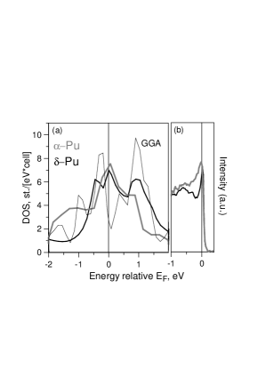
Figure 6: a) Comparison between calculated densities of states using the LDA+DMFT approach for fcc Pu: the data for $V/V_{\delta}=1.05,\,U=4.0$ eV (black line) , the data for $V/V_{\delta}=0.80,\,\,U=3.8$ eV (gray line) which correspond to the volumes of the $\delta$ and $\alpha$ phases respectively. The result of the GGA calculation (dotted line) at $V/V_{\delta}=1\,\,(U=0)$ is also given. b) Measured photemission spectrum of $\delta$ (black line) and $\alpha$ (grey line) Pu at the scale from -1.0 to 0.4 eV (after Ref. PuExp1, ).

A simple physical explanation drawn from these studies suggests that in the $\delta$ phase the f electrons are slightly on the localized side of the interaction–driven localization-delocalization transition with a sharp and narrow Kondo–like peak and well-defined upper and lower Hubbard bands. It therefore has the largest volume as has been found by previous LDA+U calculationsPuPRL ; PuLDA+U which take into account Hubbard bands only. The low-temperature $\alpha$ phase is more metallic, i.e. it has larger spectral weight in the quasiparticle peak and smaller weight in the Hubbard bands. It will therefore have a much smaller volume that is eventually reproduced by LDA/GGA calculations which neglect both Coulomb renormalizations of quasiparticles and atomic multiplet structure. The delicate balance of the energies of the two minima may be the key to understanding the anomalous properties of Pu such as the great sensitivity to small amounts of impurities (which intuitively would raise the energy of the less symmetric monoclinic structure, thus stabilizing the $\delta$ phase to lower temperature) and the negative thermal expansion. Notice however, that the $\alpha$ phase is not a weakly correlated phase: it is just slightly  displaced towards the delocalized side of the localization–delocalization transition, relative to the $\delta$ phase. This is a radical new viewpoint in the theoretical literature on Pu, which has traditionally regarded the $\alpha$ phase as well understood within LDA. However, the correlation viewpoint is consistent with a series of anomalous transport properties in the $\alpha$ phase reminiscent of heavy electron systems. For example, the resistivity of $\alpha$–Pu around room temperature is anomalously large, temperature independent and above the Mott limit PuRHO (the maximum resistivity allowed to the conventional metal). Strong correlation anomalies are also evident in the thermoelectric power PuTHERM .

V Conclusion

In conclusion, this work describes a first principles method for calculating the electronic structure of materials where many–body correlation effects between the electrons are not small and cannot be neglected. It allows simultaneous evaluation of the total free energy and the local electronic spectral density. The approach is based on the effective action functional formulation of the free energy and is viewed as spectral density functional theory. An approximate form of the functional exploits a local dynamical mean–field theory of strongly correlated systems accurate in the situations when the self–energy is short ranged in a certain portion of space. The localization is defined with reference to some basis in Hilbert space. It does not necessarily imply localization in real space and is treated using a general basis set following the ideology of the cellular dynamical mean field theory. Further approximations of the theory, such as LDA+DMFT and local GW are discussed. Implementation of the method is described in terms of the energy–dependent one–particle states expanded via the linear muffin–tin orbitals. Application of the method in its LDA+DMFT form is given to study the anomalous volume expansion in metallic Plutonium. We obtain equilibrium volume of the $\delta$ phase in good agreement with experiment with no magnetic order imposed in the calculation. The calculated one–electron densities of states are consistent with the results of the photoemission. Our most recent studies PuScience of the lattice dynamical properties of Pu address the problem of the $\delta\rightarrow\varepsilon$ transitions and show good agreement with experimentPuWong .

Alternative developments of the LDA+DMFT approach by several groups around the world discuss other applications of the dynamical mean field theory in electronic structure calculations. The results obtained are promising. Volume collapse transitions, materials near the Mott transition, systems with itinerant and local moments, as well as many other exciting problems are beginning to be explored using these methods.

The authors would like to thank for many enlightening discussions the participants of the research school on Realistic Theories of Correlated Electron Materials, Kavli Institute for Theoretical Physics, fall 2002, where the part of this work was carried out. Many helpful discussions with the participants of weekly condensed matter seminar at Rutgers University are also acknowledged. Conversations with A. Georges, A Lichtenistein, N. E. Zein related to various aspects of dynamical mean–field and GW theories are much appreciated. The authors are indebted to E. Abrahams, A. Arko, J. Joyce, H. Ledbetter, A. Migliori, and J. Thompson for discussing the issues related to the work on Pu. The work was supported by the NSF DMR Grants No. 0096462, 02382188, 0312478, 0342290,  US DOE division of Basic Energy Sciences Grant No DE-FG02-99ER45761, and by Los Alamos National Laboratory subcontract No 44047-001-0237. Kavli Institute for Theoretical Physics is supported by NSF grant No. PHY99-07949.

References

- (1) For a review, see, e.g., Theory of the Inhomogeneous Electron Gas, edited by S. Lundqvist and S. H. March (Plenum, New York, 1983).
- (2) For a review, see, e.g., F. Aryasetiawan and O. Gunnarsson, Rep. Prog. Phys. 61, 237 (1998).
- (3) See, e.g., N. E. Bickers and D. J. Scalapino, Ann. Phys. 193, 206 (1989).
- (4) For a review, see, e.g.,M. Jarrell, and J. E. Gubernatis, Physics Reports, 269, 133 (1996).
- (5) For a review, see, e.g., E. Dagotto, Rev. Mod. Phys. 66, 763 (1994).
- (6) S. R. White, Phys. Rev. Lett. 69, 2863 (1992).
- (7) For a review, see, V. I. Anisimov, F. Aryasetiawan, and A. I. Liechtenstein, J. Phys. Cond. Matter 9, 767 (1997).
- (8) See, e.g., A. Svane and O. Gunnarsson, Phys. Rev. Lett. 65, 1148 (1990); Z. Szotek, W. M. Temmerman and H. Winter, Phys. Rev. B47, 4029 (1993).
- (9) For a review, see, E. K. U. Gross, J. F. Dobson, and M. Petersilka, in Density Functional Theory, edited by R. F. Nalewajski, Springer Series Topics in Current Chemistry (Springer, Heidelberg, 1996).
- (10) For a review, see, e.g., A. Georges, G. Kotliar, W. Krauth, and M. J. Rozenberg, Rev. Mod. Phys. 68, 13 (1996).
- (11) For a review, see, e.g., H. Held, I. A. Nekrasov, G. Keller, V. Eyert, N. Blümer, A. K. McMahan, R. T. Scalettar, Th. Pruschke, V. I. Anisimov, D. Vollhardt, in Psi–k Network Newsletter, June 2003.
- (12) G. Kotliar and S. Y. Savrasov, in New Theoretical approaches to strongly correlated systems, edited by A. M. Tsvelik, (Kluwer Academic Publishers, the Netherlands, 2001), p. 259; cond–mat/020824.
- (13) S. Y. Savrasov and D. Y. Savrasov, Phys. Rev. B 54, 16487 (1996).
- (14) J. Hubbard, Proc. Roy. Soc. (London) A281, 401 (1964).
- (15) M. S. Hybertsen and S. G. Louie, Phys. Rev. B 34, 5390 (1986).
- (16) N. E. Zein, V. P. Antropov, Phys. Rev. Lett. 89,126402 (2002).
- (17) M. H. Hettler, A. N. Tahvildar-Zadeh, and M. Jarrell, T. Pruschke, H. R. Krishnamurthy, Phys. Rev. B 58, 7475 (1998).
- (18) G. Kotliar, S. Savrasov, G. Palsson, and G. Biroli, Phys. Rev. Lett. 87, 186401 (2001).
- (19) G. Biroli, O. Parcollet, G. Kotliar, cond-mat/0307587 (unpublished).
- (20) V. I. Anisimov, A. I. Poteryaev, M. A. Korotin, A. O. Anokhin, and G. Kotliar, J. Phys.: Condens. Matter 35, 7359 (1997).
- (21) A. Fujimori, I. Hase, M. Nakamura, H. Namatame, Y. Fujishima, Y. Tokura, M. Abbate, F. M. F. de Groot, M. T. Czyzyk, J. C. Fuggle, O. Strebel, F. Lopez, M. Domke, and G. Kaindl, Phys.Rev. B 46, 9841 (1992).
- (22) A. Lichtenstein and M. Katsnelson, Phys. Rev. B 57, 6884 (1998).
- (23) K. Held, G. Keller, V. Eyert, D. Vollhardt, V.I. Anisimov, Phys. Rev. Lett. 86, 5345 (2001).
- (24) A. I. Lichtenstein, M. I. Katsnelson, G. Kotliar, Phys. Rev. Lett. 87, 067205 (2001).
- (25) V. S. Oudovenko, G. Palsson, G. Kotliar, S. Y. Savrasov, cond–mat/0209336 (unpublished).
- (26) P. Sun, G. Kotliar, Phys. Rev. B 66, 085120 (2002).
- (27) S. Biermann, F. Aryasetiawan, A. Georges, Phys. Rev. Lett. 90, 086402 (2003).
- (28) M. S. Hibertsen, M. Schlüter, and N. E. Christensen, Phys. Rev. B 39, 9028 (1989); A. K. McMahan, R. M. Martin and S. Satpathy, Phys. Rev. B 38, 6650 (1988).
- (29) R. Chitra and G. Kotliar, Phys. Rev. B62, 12715 (2000).
- (30) R. Chitra and G. Kotliar, Phys. Rev. B 63, 115110 (2001).
- (31) K. Held, A.K. McMahan, R.T. Scalettar, Phys. Rev. Lett. 87, 276404 (2001).
- (32) S. Savrasov, G. Kotliar, and E. Abrahams, Nature 410, 793 (2001).
- (33) S. Y. Savrasov, G. Kotliar, Phys. Rev. Lett. 90, 056401 (2003).
- (34) X. Dai, S. Y. Savrasov, G. Kotliar, A. Migliori, H. Ledbetter, E. Abrahams, Science 300, 953 (2003).
- (35) S. Sachdev and J. Ye, Phys. Rev. Lett. 70, 3339 (1993); H. Kajueter and G. Kotliar (unpublished); H. Kajueter, PhD thesis, Rutgers University, 1995; Q. Si and J. L. Smith, Phys. Rev. Lett. 77, 3391 (1996); J. L. Smith and Q. Si, Phys. Rev. B 61, 5184 (2000).
- (36) P. W. Anderson, Phys. Rev. 124, 41 (1961).
- (37) M. Gutzwiller, Phys. Rev. 134, A923 (1964).
- (38) G. Kotliar and A. E. Ruckenstein, Phys. Rev. Lett. 57, 1362 (1986).
- (39) R. Fresard and G. Kotliar, Phys. Rev. B. 56, 12909 (1997).
- (40) W. Nolting, W. Borgiel , Phys. Rev. B 39, 6962(1989).
- (41) V. Oudovenko, S. Y. Savrasov, G. Kotliar, and D. Villani (unpublished).
- (42) O. K. Andersen, Phys. Rev. B 12, 3060 (1975).
- (43) O. K. Andersen and O. Jepsen, Phys. Rev. Lett. 53, 2571 (1984).
- (44) S. Y. Savrasov, Phys. Rev. B54, 16470 (1996).
- (45) R. Fukuda, T. Kotani, and S. Yokojima, Prog. Theor. Phys. 92, 833 (1994).
- (46) N. Argaman and G. Makov, cond–mat/9806013 (unpublished).
- (47) M. Valiev and G. Fernando, Phys. Lett. A 227, 265 (1997).
- (48) T. Plefka, J. Phys. A 15, 1971 (1982); A. Georges and J. S. Yedidia, J. Phys. A 24, 2173 (1991).
- (49) A. Georges, in Proceedings of the NATO Advanced Study Institute on Field Theory of Strongly Correlated Bosons and Fermions in Low-Dimensional Disordered systems, edited by I. V. Lerner, B. Altshuler, V. I. Fal’ko (NATO Science Series II, 2002)
- (50) J. Harris and R. O. Jones, J. Phys. F 4, 1170 (1974); O. Gunnarsson and B. I. Lundqvist, Phys. Rev. B 13, 4274 (1976); D. C. Langreth and J. P. Perdew, Phys. Rev. B 15, 2884 (1977).
- (51) A. Georges and G. Kotliar, Phys. Rev. B 45, 6479 (1992).
- (52) M. J. Rozenberg, G. Kotliar and X. Y. Zhang, Phys. Rev. B 49, 10181 (1994).
- (53) M. Springer and F. Aryasetiawan, Phys. Rev. B 57, 4364 (1998); T. Kotani, J. Phys.: Condens. Matter 12, 2413 (2000).
- (54) I.A. Nekrasov, K. Held, N. Blumer, A.I. Poteryaev, V.I. Anisimov, and D. Vollhardt, Eur. Phys. J. B18, 55 (2000).
- (55) I. Paul, et.al (unpublished).
- (56) S. Y. Savrasov, G. Kotliar, cond-mat/0106308 (unpublished).
- (57) V. I. Anisimov, J. Zaanen, and O. K. Andersen, Phys. Rev. B 44, 943 (1991).
- (58) I. I. Mazin, A. G. Petukhov, L. Chioncel and A. I. Lichtenstein, Phys. Rev. B 67, 153106 (2003).
- (59) S. Savrasov and G. Kotliar, Phys. Rev. Lett. 84, 3670 (2000).
- (60) N. E. Zein , et.al (unpublished).
- (61) Ph. Lambin and J. P.Vigneron, Phys. Rev. B 29, 3430 (1984).
- (62) For a review, see e.g., The Actinides: Electronic Strucuture and Related Properties, edited by A. J. Freeman and J. B. Darby, Vols. 1 and 2 (Academic Press, New York, 1974).
- (63) S. S. Hecker, L. F. Timofeeva, Los Alamos Science 26, 244 (2000).
- (64) A. M. Boring and J. L. Smith, Los Alamos Science 26, 91 (2000).
- (65) A.J. Arko, J.J. Joyce, L. Morales, J. Wills, and J. Jashley, Phys. Rev. B62, 1773 (2000).
- (66) I. V. Solovyev, A. I. Liechtenstein, V. A. Gubanov, V. P. Antropov, and O. K. Andersen, Phys. Rev. B43, 14414 (1991).
- (67) For recent calculations, see, P. Söderlind, O. Eriksson, B. Johansson, and J. M. Wills, Phys. Rev. B50, 7291 (1994); M. D. Jones, J. C. Boettger, R. C. Albers, and D. J. Singh, Phys. Rev. B61, 4644 (2000).
- (68) J. Bouchet, B. Siberchicot, F. Jollet, and A. Pasturel, J. Phys.: Condens. Matter 12, 1 (2000).
- (69) P. Söderlind, Europhys. Lett. 55, 525 (2001).
- (70) O. Eriksson, J. D. Becker, A. V. Balatsky, and J. M. Wills, J. Alloys and Comp. 287, 1 (1999).
- (71) L.Petit, A.Svane, W.M.Temmerman, and Z.Szotek, Solid State Commun. 116, 379 (2000); A. Setty and B. R. Cooper, in Bulletin of March Meeting of American Physical Society (2003), abstract G15.007.
- (72) W. Harrison, Phil. Mag. B 82, 1755 (2002).
- (73) B. Johansson, Phil. Mag. 30, 469 (1974).
- (74) S. Florens, A. Georges, G. Kotliar, O. Parcollet, Phys. Rev. B 66, 205102 (2002).
- (75) H. J. Vidberg and J.W. Serene, Journal of Low Temperature Physics, 29, 179 (1977).
- (76) J. P. Perdew, K. Burke, and M. Ernzerhof, Phys. Rev. Lett. 77, 3865 (1996).
- (77) J. P. Desclaux and A. J. Freeman, in Handbook on the Physics and Chemistry of the Actinides, edited by A. J. Freeman and G. H. Lander (Elsevier, Amsterdam, 1984), Vol. 1.
- (78) P. E. A. Turchi, A. Gonis, N. Kioussis, D. L. Price, B. R. Cooper, in Proceedings of the International Workshop on Electron Correlations and Materials Properties, edited by A. Gonis, N. Kioussis, and M. Ciftan, Kluwer Academic, New York, 1999, p. 531.
- (79) See, e.g., G. Kotliar, S. Murthy, M. J. Rozenberg, Phys. Rev. Lett. 89, 046401 (2002).
- (80) R. Lallement, J. Phys. Chem. Solids 24, 1617 (1963).
- (81) J. Wong, M. Krisch, D. L. Farber, F. Occelli, A. J. Schwartz, T.–C. Chiang, M. Wall, C. Boro, and R. Xu, Science, in press (2003).