Two dimensional electron gas near full polarization

Abstract

We establish the consistency of the Fermi liquid description and find a relation between Fermi liquid constants for the two dimensional electron system near the point of full polarization due to a parallel magnetic field $H$. Our results enable us to predict connections between different thermodynamic properties of the system. In particular, we find that near the point of full polarization $H_{c}$, the thermodynamic compressibility of the system experiences a jump with the subleading $(H_{c}-H)^{1/2}$ dependence on the magnetic field. Also, the magnetization has a cusp with the dependence of the type $(H-H_{c})+(H_{c}-H)^{3/2}$ at $H<H_{c}$.

I Introduction

The appearance of the new generation of high mobility heterostructures pfeiffer resulted in observations of interesting phenomena effects ; du ; sivan which brought new spotlight on the effects of strong interactions in two-dimensional electron systems (2DES). For us this renews theoretical interest in the thermodynamical properties of clean Fermi liquids.

Traditional theoretical description of 2DES is based upon the theories of weakly interacting Fermi gas ando and Landau Fermi liquid theory landau ; AGD . In the limit of very strong interactions (corresponding to low electron densities) such a description breaks down. However the situation changes if the low density 2DES interacts with another 2DES with much higher density. In this paper we present an example where this coexistance naturally occurs as a result of a strong spin polarization of a 2DES due to a high in-plane magnetic field. We find a consistent Landau Fermi liquid description for this system (despite the fact that a naive estimate of the plasma parameter $r_{s}$ for the minority spin component yields a formally large value). The remarkable feature of our result is that in the close vicinity of the spin polarized state the perturbative expansion is possible in terms of the inverse gas parameter of the low density subsystem. This enbles us to determine the functional form of the dependencies of the 2DES compressibility, magnetization, and specific heat on the small density of the minority electrons.

To understand the relation of this problem to the Fermi liquid theory at zero field let us recall the basic structure of the quasiparticle interaction functional (we will not write the trivial long-range Coulomb interaction term)

$${\cal H}_{\rm int}=\frac{1}{2}F^{\rho}\rho^{2}+\frac{1}{2}\sum_{\alpha,\beta=x,y,z}F^{\sigma}_{\alpha\beta}S^{\alpha}S^{\beta},$$ (1)

where $\rho$ is the charge density, $S^{x,y,z}$ denote components of the spin density, and $F^{\rho},\ \hat{F}^{\sigma}$ are the corresponding Fermi liquid parameters. The charge (singlet channel) and the spin (triplet) fluctuations are decoupled, and $SU(2)$ symmetry of the system guarantees $F^{\sigma}_{\alpha\beta}=F^{\sigma}\delta_{\alpha\beta}$.

If the magnetic field is applied along, say, the $x$ - direction (in the plane of the 2DES), the $SU(2)$ symmetry is reduced to $U(1)$ and one may write for the quadratic part of the energy

$${\cal H}_{\rm int}=\frac{F^{\rho}}{2}\rho^{2}+\frac{F^{\sigma}_{\parallel}}{2}\left[S^{x}\right]^{2}+{F^{\sigma\rho}}\rho S^{x}+\frac{F^{\sigma}_{\perp}}{2}\sum_{\alpha=y,z}S^{\alpha}S^{\alpha}.$$ (2)

This means that the system can no longer be described by two constants. Now the reduced symmetry allows for four independent parameters.

Simplifications are possible, however, with the further increase of the magnetic field, because oscillations of the spin density components $S_{y,z}$ become gapped (the gap equals to the Zeeman splitting $E_{z}$). Therefore, for the description of low lying excitations with the energy much smaller than $E_{z}$, the last term in Eq. (2) can be ignored. Introducing deviations of densities of majority (minority) electrons $n_{1(2)}=\rho/2\pm S_{x}/2$, one obtains the two-fluid model

$${\cal H}_{\rm int}=\frac{F_{11}}{2}n_{1}^{2}+\frac{F_{22}}{2}n_{2}^{2}+F_{12}n_{1}n_{2}$$ (3)

characterized by three independent parameters.

Equation (3) suggests two questions: (i) what is the lowest density of minority electrons for which it is applicable; and (ii) whether the three constants of the model are indeed independent. The ultimate goal of this paper is to show that (i) the Fermi liquid description is consistent for any density of the minority electrons and (ii) there is a relation between the Fermi liquid constants for the vanishing density of the minority electrons. The only requirement for this description to be valid is that the fully polarized electron system is a stable Fermi liquid. The remarkable feature of this result is that in the close vicinity of the spin polarized state the perturbative expansion in terms of the inverse gas parameter $\hbar v_{F2}/e^{2}$ is possible (here $v_{F2}$ is the Fermi velocity of the minority electrons).

The remainder of the paper is organized as follows. In Section II we give a phenomenological description of the system near full polarization, present the main results and predict connections between different thermodynamic properties of the system. Section III contains the microscopic derivation (justification) of the announced results, first in an intuitive, then in Subsections III.2 and III.3, in a more rigorous manner.

II Phenomenology near full polarization

II.1 Structure of the theory

Let us consider the system first at zero temperature. Because the total spin of the system commutes with the Hamiltonian, we can write the energy density of the system $\delta{\cal H}$ in terms of the majority ($n_{1}$) and minority electron density ($n_{2}$). Omitting the trivial term of the direct Coulomb interaction (we will work with fixed total density $n_{1}+n_{2}=N$), one finds

$${\cal H}=\frac{1+F_{11}}{2\nu_{1}}\delta n_{1}^{2}+{\cal H}_{2}(n_{2},N)+\frac{F_{12}}{{\nu_{1}}}n_{2}\delta n_{1}-$$

$$\quad\quad-\frac{E_{z}-E_{z}^{c}(N)}{2}\left(\delta n_{1}-n_{2}\right)-\frac{E_{z}}{2}N.$$ (4)

The first term in Eq. (II.1) is the quadratic expansion of the ground state energy of the fully spin polarized electron system, $n_{1}=N$. It has the standard Fermi-liquid form with $\nu_{1}$ being the density of states (entering the slope of the specific heat). The second term ${\cal H}_{2}$ characterizes the energy of the minority electrons at fixed $n_{1}=N$ and the third term characterizes the change in this energy due to modification of the majority density. The last two terms characterize the shift of the energies due to the magnetic field, $H$, and $E_{z}=g\mu_{B}H$ is the bare Zeeman splitting, with $g$ being the bare (non-renormalized by electron-electron interaction) Lande $g$-factor, and $\mu_{B}$ being the Bohr magneton. The quantity $E_{z}^{c}(N)$ corresponds to the value of the magnetic field above which the magnetization is independent of the field. In other words, this value limits from above the region of the field where the finite density of the minority electrons is still energetically profitable.

In order to find the ground state of the whole system we have to minimize energy Eq. (II.1) with respect to the electron densities. Having in mind that the total electron density is fixed by an external gate, we note that the densities are coupled by the constraint

$$\delta n_{1}+n_{2}=\delta N,\quad n_{2}\geq 0,$$ (5)

where $\delta N$ is the change in the total electron density with respect to the density threshold for the population of the minority subband controllable by the variation of the gate voltage. This yields either $n_{2}=0$ or

$$0=\frac{\partial{\cal H}_{2}(n_{2},N)}{\partial n_{2}}+\left[E_{z}-E_{z}^{c}(N)\right]+$$ (6)

$$\quad\quad+\frac{1+F_{11}}{\nu_{1}}\left(n_{2}-\delta N\right)-\frac{F_{12}}{\nu_{1}}\left(2n_{2}-\delta N\right).$$

The crititical field $E_{z}^{c}(N+\delta N)$ is determined as the field at which $n_{2}=0$ solves Eq. (6). Then the first term vanishes (see below) and we obtain

$$\frac{\partial E_{z}^{c}}{\partial N}=\frac{1+F_{11}-F_{12}}{\nu_{1}}.$$ (7)

Further progress requires knowledge of the function ${\cal H}_{2}(n_{2},N)$. We find

$${\cal H}_{2}(n_{2},N)=\int\limits_{0}^{n_{2}}dn^{\prime}\int\limits_{0}^{n^{\prime}}dn^{\prime\prime}\left[\frac{1}{\nu_{2}(n^{\prime\prime},N)}+\frac{F_{22}(n^{\prime\prime},N)}{\nu_{1}(N)}\right],$$ (8a)

where the dependence of the density of states of the electron density is given by

$$\frac{1}{\nu_{2}(n,N)}=\frac{1}{\nu_{2}(N)}+$$ (8b)

$$\quad\quad+\frac{4\sqrt{\pi n}[1+F_{11}(N)-F_{12}(N)]^{2}}{3e^{2}\pi^{2}\left[\nu_{1}(N)\right]^{2}}+{\cal O}\left(\frac{n}{N}\ln\frac{n}{N}\right),$$

and the Fermi liquid constant for the minority electrons is

$$F_{22}(n,N)=-\left[1+F_{11}(N)-2F_{12}(N)\right]+$$ (8c)

$$\quad+\frac{4\sqrt{\pi n}[1+F_{11}(N)-F_{12}(N)]^{2}}{e^{2}\pi^{2}\nu_{1}(N)}+{\cal O}\left(\frac{n}{N}\ln\frac{n}{N}\right).$$

Equations (8) constitute the key point of this paper. They state, that properties of the minority electrons can be expressed in terms of the density of states $\nu_{2}(N)\equiv\nu_{2}(n_{2}=0,N)$ at the point of full polarization (renormalized by interaction with the majority electrons) and the Fermi liquid constants, $F_{11},\ F_{12}$ of the majority electrons. We will see below that the above equations impose certain connections between different observable quantities. It is interesting to notice that the relevant expansion parameter here is not the strength of the Coulomb interaction, $e^{2}$, but rather its inverse power. This expansion is valid for $n_{2}a_{B}^{2}\ll 1$, where $a_{B}$ is the usual screening radius in two dimensions, $a_{B}\simeq 1/\nu_{1}e^{2}$.

Postponing a rigorous derivation of Eqs. (8) until the next section, we discuss their physical meaning. Consider $n_{2}\to 0$ and retain only the first line in Eq. (8c). Substituting the result into Eqs. (8a) and (II.1) and keeping only quadratic terms we find

$${\cal H}=\frac{n_{2}^{2}}{2\nu_{2}}+\frac{\left(1+F_{11}\right)}{2\nu_{1}}\left(\delta n_{1}^{2}-n_{2}^{2}\right)+\frac{F_{12}}{{\nu_{1}}}n_{2}\left(n_{2}+\delta n_{1}\right).$$

Let us now set $\delta n_{1}=-n_{2}$ (keeping electrical neutrality). The Hamiltonian takes the form

$${\cal H}=\frac{n_{2}^{2}}{2\nu_{2}},$$

which correponds to the compressibility of non - interacting minority electrons. This is not accidental; the majority electrons screen the Coulomb interaction at distances of the order of the screening radius. At small densities, however, the distance between minority electrons is much larger than this radius. Therefore, this screened interaction is seen by minority electrons only as contact interaction, i.e. the effect of this interaction vanishes because of the Pauli principle. This explains the origin of the first line in Eq. (8c). The second term in Eq. (8c) describes the effect of the finite interaction range. This effect clearly vanishes as the distance between minority electrons increases. Because the residual interaction is of the dipole type $U_{sc}(r)\simeq e^{2}a_{B}^{2}/r^{3}$, its effect can be estimated as $\delta{\cal H}\simeq U_{sc}(r=1/\sqrt{n_{2}})n_{2}$ which immediately gives a $\sqrt{n_{2}}$ dependence to the Fermi liquid parameter $F_{22}$. As a matter of fact, the same $\sqrt{n_{2}}$ arises in all angular harmonics of $F_{22}$ (and $F_{12}$ as well; see the following section). This leads to renormalization of the effective mass and, therefore, the density of states in Eq. (8b). The residual interaction is weak and therefore the perturbative treatment of the minority electrons is legitimate.

To complete the calculation of the ground state energy, we use Eqs. (8) in Eq. (6) and find with the help of Eq. (7)

$$n_{2}=n_{0}\left[1-\gamma R_{s}n_{0}^{1/2}+\dots\right];$$ (9)

$$R_{s}=\frac{1}{e^{2}\nu_{2}}\left(\nu_{2}\frac{\partial E_{z}^{c}}{\partial N}\right)^{2};$$

$$n_{0}=\nu_{2}(N)\left[E_{z}^{c}(N+\delta N)-E_{z}\right]\theta\left(E_{z}^{c}(N+\delta N)-E_{z}\right)$$

Here $\theta(x)$ is the step function, and

$$\gamma=\frac{32}{9\pi^{3/2}}=0.639\dots$$ (10)

is a numerical coefficient. It is noteworthy that the subleading term in this dependence is singular near $E_{z}=E_{z}^{c}$. Substituting Eq. (9) into Eqs. (8) and the result into Eq. (II.1), we find for the ground state energy ${\cal E}$

$${\cal E}=\frac{1+F_{11}}{2\nu_{1}}\delta N^{2}-\frac{E_{z}N}{2}-\frac{n_{0}^{2}}{2\nu_{2}}+\frac{2}{5}\frac{\gamma R_{s}n_{0}^{5/2}}{\nu_{2}},$$ (11)

where we omitted terms linear in $\delta N$ (apart from the term proportional to $E_{z}$) as they will not contribute to the observable quantities discussed in the following subsection.

II.2 Experimental consequences.

In this subsection we apply the above ideas to establish relations between different thermodynamic properties of the system near the point of full polarization.

The leading contribution to the specific heat of the two-liquid system is simply the sum of the quasiparticle specific heats of the two species of electrons,

$$\left(\frac{\partial C_{V}}{\partial T}\right)_{T\to 0}=\frac{\pi^{2}\nu_{1}(N)}{3}+$$ (12)

$$\quad\quad+\frac{\pi^{2}\nu_{2}(N)}{3}\left[1-\left(\frac{3\gamma^{2}R_{s}^{2}\nu_{2}\delta E_{z}}{8}\right)^{\frac{1}{2}}\right]\theta\left(\delta E_{z}\right);$$

$$\quad\quad\quad\quad\quad\delta E_{z}=E_{z}^{c}(N)-E_{z}.$$

This gives the operational definition of the density of states, even though the actual measurement of the specific heat in two dimensions is technically difficult.

Next, Eq. (7) allows one to find a certain combination of the Fermi-liquid constants $1+F_{11}-F_{12}$ from the measurement of the critical magnetic field as a function of electron density.

Further information about the Fermi liquid constants can be obtained from studying the thermodynamic compressibility $\kappa=(\partial^{2}{\cal E}/\partial^{2}N)^{-1}$, where ${\cal E}$ is the ground state energy of the system. Differentiating Eq. (11) yields

$$\frac{1}{\kappa}=\frac{1+F_{11}}{\nu_{1}}-e^{2}R_{s}\left(1-\frac{3\gamma}{2}\sqrt{R_{s}^{2}\nu_{2}\delta E_{z}}\right)\theta\left(\delta E_{z}\right).$$ (13)

We see that the measurement of the jump in the compressibility gives the value of the parameter $R_{s}$ which together with Eq. (9) and measurements of $\partial_{N}E_{z}^{c}(N)$ yields the value of $\nu_{2}(N)$ without specific heat measurements. After that the coefficient in front of subleading square-root singularity does not contain any fitting parameters.

Finally, we calculate the magnetizetion $M=-\partial_{H}{\cal E}$ as the function of magnetic field $H$. Differentiating Eq. (11) at $\delta N=0$ with the help of Eq. (9), we obtain

$$M=g\mu_{B}\left[\frac{N}{2}-\nu_{2}\delta E_{z}\left(1-\gamma\sqrt{R_{s}^{2}\nu_{2}\delta E_{z}}\right)\theta\left(\delta E_{z}\right)\right].$$ (14)

It is important to emphasize that after the compressibility and $M$ at $E_{z}>E_{z}^{c}$ are measured, the formula for magnetization at $E_{z}<E_{z}^{c}$ will not have any adjustable parameters. It is also worth noticing that the sub-leading dependence has a square root singularity, similar to that in Eq. (13).

The predicted dependencies of magnetization and compressibility are plotted on Fig. 1.

Figure 1: Predicted dependences of compressibility (dashed-dotted line) and susceptibility (solid line).

III Microscopic derivation

The purpose of this section is to develop the microscopic description leading to Eqs. (8), which is needed to justify the Fermi liquid description of the minority electrons and to calculate the coefficient in the second term of Eqs. (8b) and (8c). The form of the first term in Eq. (8c) follows already from the physical argument presented after Eq. (8c) and it will also be confirmed by the microscopic calculation.

The route we are taking in this section is the following. First, we express our physical arguments in the language of the perturbation theory, i.e. identify the set of diagrams leading to Eqs. (8). The rest of the derivation aims at showing that (i) these are the only diagrams that produce a combination of the constant ($n_{2}=0$ term) and the term with $\sqrt{n_{2}}$ singularity, (ii) all other diagrams result in contributions of the order of $(n_{2}/N)\ln n_{2}/N$; (iii) the Fermi liquid description of the minirity electrons is justified. This material will be structured into subsections III.1, III.2 and III.3. The rather cumbersome content of these subsections will not directly contribute to the final results and might be skipped by a pragmatic reader.

III.1 Perturbation theory

The goal of the microscopic consideration presented in this section is to prove the main assumption of the phenomenological treatment, namely Eqs. (8). We start by showing how one can arrive at Eqs. (8) using a simple-minded perturbative approach. The reason to do this is to build up physical intuition, identify the group of diagrams which gives the dominant contribution to the minority electron interaction, and to clarify the assumptions, which one needs to make in order to justify this treatment. In the following two subsections we shall prove the validity of these assumptions and provide a more rigorous treatment of the problem.

The main physical idea of the following picture is that close to the point of full polarization only the majority electrons participate in screening. Therefore, as a building block for the perturbation theory we are going to use the dynamically screened (by the majority electrons) Coulomb interaction, which propagator has a diagrammatic representation of Fig. 2. The corresponding analytic expression is

$$V(\omega,q)=\frac{V_{0}(q)}{1+V_{0}(q)\Pi_{1}\left(\omega,q\right)},$$ (15)

where $V_{0}(q)=2\pi e^{2}/|q|$ is the bare Coulomb interaction and $\Pi_{1}\left(\omega,q\right)$ is the polarization operator of the majority system. It is defined as the part of the density - density correlation function irreducible with respect to one Coulomb line. For small momentum and frequency transfers, $q,\omega/v_{F1}\ll p_{F1}$, it has the usual Fermi-liquid form AGD

$$\Pi_{1}\left(\omega,q\right)=\int\frac{d\phi_{1}d\phi_{2}}{(2\pi)^{2}}\Pi_{1}\left(\omega,{\bf q};{{\bf n}}_{1},{{\bf n}}_{2}\right);$$ (16)

$$\Pi_{1}\left(\omega,{\bf q};{{\bf n}}_{1},{{\bf n}}_{2}\right)=\Pi_{1}^{qp}\left(\omega,{\bf q};{{\bf n}}_{1}\right)2\pi\delta(\phi_{1}-\phi_{2})-$$

$$-\int\frac{d\phi_{3}}{2\pi}\Pi_{1}^{qp}\left(\omega,{\bf q};{{\bf n}}_{1}\right)\frac{F_{11}\left(\widehat{{\bf n}_{1}{\bf n}_{3}}\right)}{\nu_{1}}\Pi_{1}\left(\omega,{\bf q};{{\bf n}}_{3},{{\bf n}}_{2}\right);$$

$$\Pi_{1}^{qp}\left(\omega,{\bf q};{{\bf n}}\right)=\frac{\nu_{1}v_{F1}{{\bf n}}\cdot{\bf q}}{v_{F1}{{\bf n}}\cdot{\bf q}-\omega-i0\mbox{sgn}\omega}.$$ (17)

Here $F_{11}\left(\widehat{{\bf n}_{1}{\bf n}_{2}}\right)$ is the majority Fermi liquid parameter (taken at zero minority density $n_{2}=0$), $\Pi_{1}^{qp}\left(\omega,q;{{\bf n}}\right)$ characterizes the linear response of non-interacting quasiparticles, and $\nu_{1}$ is the density of states of majority quasiparticles. The latter quantity enters into the specific heat of the spin polarized ($n_{2}=0$) system. Equation (16) takes into account all possible contributions singular as a function of $v_{F1}q/\omega$ and neglects all the contributions which are regular functions of the parameters $(q/p_{F1})^{2}$ and $\omega/\epsilon_{F1}$. Unit vectors ${\bf n}_{i}=(\cos\phi_{i},\sin\phi_{i})$ characterize the direction of motion of the quasiparticle.

Now we discuss the origin of Eqs. (8).

Figure 2: Dyson equation for the dynamical screening by majority electrons.

III.1.1 Interaction of minority electrons

To justify the relation Eq. (8c) we need to describe the interaction of minority electrons in terms of the parameters of majority electrons. Since interaction between minority electrons is characterized by the energy transfer $\omega\simeq qv_{F2}\ll qv_{F1}$, we can use the static approximation for $V(\omega,q)$. Moreover, at wavectors smaller than the inverse screening radius of majority electrons $\nu_{1}V_{0}(q)\gg 1$. In this case Eq. (15) becomes (see subsection III.2 for further discussions)

$$V\left(\omega,q\right)\approx\frac{1}{\nu_{1}}\left[1+F_{11}^{(0)}-\frac{\left(1+F_{11}^{(0)}\right)^{2}}{\nu_{1}V_{0}(q)}+\dots\right].$$ (18)

Here we use angular harmonics of the Fermi liquid functions

$$F_{ij}\left(\phi\right)=\sum_{m}e^{im\phi}F_{ij}^{(m)},$$ (19)

for $i,j=1,2$. The zeroth angular harmonics, $F_{ij}^{(0)}$, that appear in Eq. (18) correspond to the constants used in the previous sections.

Figure 3: Leading contribution to $F_{22}$.

The lowest order contribution to the minority electron interaction (that determines the Fermi liquid constant $F_{22}$) is given by the diagram in Fig. 3. Using Eq. (18) to evaluate this contribution we find

$${\rm Fig}.~{}\ref{F22first}.=-\frac{1+F_{11}^{(0)}}{\nu_{1}}+\frac{\left(1+F_{11}^{(0)}\right)^{2}}{\nu_{1}^{2}V_{0}(|{\bf p}_{1}-{\bf p}_{2}|)}\dots.$$ (20)

This contribution is proportional to $|{\bf p}_{1}-{\bf p}_{2}|\sim p_{F2}\propto\sqrt{n_{2}}$ which produces the singular density dependence in Eq. (8c).

We now show that higher order diagrams built out of the same ingredients as the simplest diagram in Fig. 3 depend on at least the second power of $|{\bf p}_{1}-{\bf p}_{2}|$ and thus result only in regular contributions to $F_{22}$.

Indeed, summation of the ten second order diagrams in Fig. 4 yields zero whenever one of the dashed lines is substituted with a constant. Therefore, the constant part of the potential Eq. (18) can be omitted entirely from the second order perturbation theory and one obtains

$${\rm Fig}.~{}\ref{F22second}.\ {\rm(a)}+\dots+{\rm(g)}\propto\left[\frac{\left(1+F_{11}^{(0)}\right)^{2}}{\nu_{1}^{2}V_{0}(p_{12})}\right]^{2}\propto(p_{12})^{2};$$

$$\quad\quad\quad p_{12}=|{\bf p}_{1}-{\bf p}_{2}|.$$

This cancellation is not accidental and in fact is due to the Fermi statistics of the minority electrons. All higher order terms are canceled in the same manner.

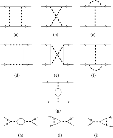
Figure 4: Connected second-order minority diagrams (all solid lines denote Green’s functions of minority electrons).

Unfortunately, this is still not the whole story. Majority electrons affect minority electrons not only through the density-density interaction but also through the renormalization of the spectrum of minority electrons (the simplest analogy here is the polaronic shift of the bottom of the minority band). This renormalization depends on the distribution function of majority electrons and, therefore, generates the Fermi liquid function $F_{12}$. The lowest order diagrams for this parameter are shown in Fig. 5. Precisely the same diagrams enter into the two particle irreducible vertex (that contributes to $F_{22}$) in Fig. 6. Therefore, this so far neglected contribution to the minority interaction can be expressed entirely in terms of $F_{12}$ (by means of direct comparison with diagrams in Fig. 5). We find

$${\rm Fig}.~{}\ref{alles}.(a)=\frac{[F_{12}^{(0)}]^{2}}{\nu_{1}^{2}}\Pi_{1}(0,p_{12})=\frac{[F_{12}^{(0)}]^{2}}{\nu_{1}(1+F_{11}^{(0)})}$$ (21a)

$${\rm Fig}.~{}\ref{alles}.(b)=-\frac{[F_{12}^{(0)}]^{2}}{\nu_{1}^{2}}\Pi_{1}(0,p_{12})^{2}V(0,p_{12})$$ (21b)

$$\hskip 44.10185pt=-\frac{[F_{12}^{(0)}]^{2}}{\nu_{1}(1+F_{11}^{(0)})}+\frac{[F_{12}^{(0)}]^{2}}{\nu_{1}^{2}V_{0}(p_{12})}$$

$${\rm Fig}.~{}\ref{alles}.(c)={\rm Fig}.~{}\ref{alles}.(d)=F_{12}^{(0)}\Pi_{1}(0,p_{12})V(0,p_{12})$$

$$\hskip 44.10185pt=\frac{F_{12}^{(0)}}{\nu_{1}}\left[1-\frac{1+F_{11}^{(0)}}{\nu_{1}V_{0}(p_{12})}\right]$$ (21c)

The reason that only the zeroth harmonics of the Fermi liquid parameters appear in Eq. (21) is that we assume: (i) $F_{12}^{(0)}\approx const+{\cal O}(q^{2}/p_{F1}^{2})$ (where $q$ is the transmitted wavevector); (ii) $F_{12}^{(1)}\sim{\cal O}(q/p_{F1})$. The dependence of $q$ on the scale of the order of $p_{F1}$ can be neglected because it would generate smallness of the order of $n_{2}/N$.

Finally, to obtain the Fermi liquid parameter $F_{22}$ we combine the two-particle irreducible minority vertex functions discussed above:

$$\frac{F_{22}(\theta)}{\nu_{1}}={\rm Fig}.~{}\ref{F22first}+{\rm Fig}.~{}\ref{alles}(a)+\dots+(d)\Big{|}_{\begin{matrix}|{\bf p}_{i}|=p_{F2};\cr\widehat{{\bf p}_{1}{\bf p}_{2}}=\theta,\end{matrix}}$$

where $i=1,2$. Summing up contributions of Eq. (21) and (20) we obtain the angle-dependent Fermi liquid parameter $F_{22}$

$$F_{22}(\theta)=-\left[1+F_{11}^{(0)}-2F_{12}^{(0)}\right]+\frac{[1+F_{11}^{(0)}-F_{12}^{(0)}]^{2}}{\nu_{1}V_{0}(2p_{F2}\sin\frac{\theta}{2})}.$$ (22)

The zeroth angular harmonic of Eq. (22) gives precisely Eq. (8c), if we recall the Landau theorem that relation $n_{2}=p_{F2}^{2}/4\pi$ is not changed by interaction in any order of the perturbation theory.

Figure 5: Lowest order diagrams for $F_{12}$.

III.1.2 Density of states of minority electrons

In order to determine the DoS (or the effective mass) of minority quasiparticles, let us recall Galilean invariance, which results in the following two-liquid variant of the usual Ward identity

$$\frac{1}{m_{2}(n)}=\frac{1}{m}-\frac{1}{m_{1}}\int\frac{d\theta}{2\pi}\left\{\frac{p_{F1}}{p_{F2}}F_{12}(\theta)+F_{22}(\theta)\right\}\cos(\theta),$$ (23)

where $m$ is the bare (band) electron mass, and $m_{1}$ is the majority quasiparticle mass. At zero minority density $F_{12}$ renormalizes the mass by the amount of order one [since the large factor $p_{F1}/p_{F2}$ cancels exactly due to the assumptions that we made deriving Eqs. (21); see the assumption (ii) in the paragraph followingEqs. (21)]:

$$\frac{1}{m_{2}(0)}=\frac{1}{m}-\frac{1}{m_{1}}\lim_{p_{F2}\to 0}\frac{p_{F1}}{p_{F2}}\int\frac{d\theta}{2\pi}F_{12}(\theta)\cos(\theta).$$ (24)

After the cancellation of the prefactor the remaining dependence of $F_{12}^{(1)}$ on $n_{2}$ is analytic. Hence, this term does not produce any singular dependence of the minority DoS on $n_{2}$. The square root dependence is caused entirely by the interaction between minority electrons, i.e. $F_{22}$. By plugging in Eq. (22) to Eq. (23) and using Eq. (24) one immediately retrieves the DoS Eq. (8b).

Figure 6: Contributions to $F_{22}$ from the renormalization of the minority spectrum.

III.1.3 Underlying assumptions

The line of argument presented so far relies on several assumptions which require further justification. These include: (i) the momentum dependence of $F_{12}$ was assumed to have the specific form (see the text following Eqs. (21); (ii) the screened interaction $V(\omega,{\bf q})$ was only considered in the limit of small frequencies, based on the intuitive assumption $\omega\simeq v_{F2}q\ll v_{F1}q$ [see text preceding Eq. (18)]; (iii) the consideration of minority interaction was limited to certain class of diagrams, see above.

The assumption (i) allowed for the explicit result Eq. (22) that followed from the evaluation of the diagrams in Figs. 3 and 6. The essence of the assumption (iii) is that no other diagram contributes to the singular dependence of $F_{22}$. Partially this was illustrated by considering diagrams in Fig. 4, however, one could imagine more complicated diagrams involving majority electrons. Moreover, the cancellation of diagrams in Fig. 4 relied heavily on the assumption (ii). Thus, in order to rigorously prove our conjecture Eqs. (8) we need to justify the above assumptions. Although proper consideration of these issues will not change the final results, we include the following subsections in order to complete the derivation.

Our strategy will be the following. First, we will set the number of minority electrons $n_{2}$ to zero inside diagrams in consideration, and discuss the analytic and scaling properties of the self-energy and $n$-point irreducible vertex functions. We will see that apart from a well-defined subclass of minority 2-particle vertices, (providing us with the nonanalytic dependence for $F_{22}$), all n-point functions are smooth (i.e. Taylor-expandable) as a function of external momenta. Second, we will treat $n_{2}\ll N$ as a perturbation and show that this may introduce only corrections linear in the small parameter $n_{2}/N$. We will use the vertex functions and the gauge invariance of the theory to calculate the Fermi liquid constant $F_{22}$ in terms of the Fermi-liquid parameters of majority spin and obtain Eq. (22). Finally, we will justify the calculation of the minority mass in more detail.

III.2 Completely polarized system

In this subsection we discuss the properties of the irreducible vertex functions which we shall use in the following subsection to calculate the Fermi liquid parameters.

III.2.1 Green functions

We start by defining zero-temperature, real time Green functions of minority ($j=2$) or majority ($j=1$) electrons:

$$\langle T_{t}\hat{\psi}_{j}({\bf R}_{1})\hat{\psi}_{k}^{\dagger}({\bf R}_{2})\rangle$$ (25)

$$\quad=i\delta_{jk}\int\frac{d^{3}P}{(2\pi)^{3}}e^{-i{\bf P}({\bf R}_{1}-{\bf R}_{2})}G_{j}({\bf P}),$$

where all the operators are taken in the Heisenberg representation and averaging is performed over the ground state of the system. To shorten the notation we use hereinafter the $(1+2)$-dimensional vectors ${\bf R}\equiv(t,{\bf r})$ and ${\bf P}\equiv(\epsilon,{\bf p})$ with the scalar product ${\bf P}{\bf R}=\epsilon t-{\bf p}{\bf r}$. There are no Green functions mixing the electron species because the electron spin component along the magnetic field is conserved.

Let us set the number of minority electrons $n_{2}$ to zero. For majority electrons we will need only the linearized spectrum near the energy shell:

$$G_{1}(\epsilon,{\bf p})=\frac{Z_{1}}{\epsilon-\xi_{1}-\Sigma_{1}\left(\displaystyle\frac{\epsilon}{v_{F1}p_{F1}},\displaystyle\frac{\xi_{1}}{v_{F1}p_{F1}}\right)},$$ (26)

where $\xi_{1}=v_{F1}\left(|{\bf p}|-p_{F1}\right)$ is the distance from the Fermi surface, $Z_{1}$ is the quasiparticle weight, $v_{F1}$ is the Fermi velocity renormalized by interaction, and $p_{F1}$ is the Fermi momentum. The relation $[p_{F1}]^{2}=4\pi n_{1}$ ($n_{1}$ being the density of majority electrons) is not affected by interaction due to the conservation of the number of states and the spin conservation (Landau theorem). The remainder of the self-energy for the majority electrons possesses the following property:

$$\Sigma_{1}(x,y)={\rm Re}\Sigma_{1}(x,y)+i\mbox{sgn}x\ \left|{\rm Im}\Sigma_{1}(x,y)\right|.$$ (27)

The leading dependence of the self-energy in two dimesnions is $\Sigma_{1}(x,x)\simeq i|x|x\ln(1/|x|)$.

As usual in Fermi liquid theory, the leading non-analytic dependences of vertex functions orginate from the overlap of poles of two Green functions with close momenta. In this case we will use the standard representation

$$G_{1}\left({\bf P}+\frac{{\bf Q}}{2}\right)G_{1}\left({\bf P}-\frac{{\bf Q}}{2}\right)$$ (28)

$$\quad\quad=2i\pi Z_{1}^{2}\delta(\epsilon)\delta(\xi)\frac{\Pi_{1}^{qp}\left(\omega,q;{{\bf n}}\right)}{\nu_{1}}+\varphi({\bf P},{\bf Q}),$$

where 2+1 vector ${\bf Q}=(\omega,\ {\bf q})$ is small in comparison with the Fermi momentum, ${\bf n}={\bf p}/|p|$ is the unit vector along the momentum ${\bf p}$, and $\varphi({\bf P},{\bf Q})$ is a smooth function with well defined limit at ${\bf Q}\to 0$. The quasiparticle polarization operator was defined in Eq. (17).

The minority electrons are described in a similar manner with the exception that now the spectrum cannot be linearized:

$$G_{2}(\epsilon,{\bf p})=\frac{1}{\epsilon-\frac{p^{2}}{2m}-\Sigma_{2}(\epsilon,{\bf p})},$$ (29)

where $m$ is the bare mass of the electron and $\Sigma_{2}$ is the self-energy of minority electrons. Because $n_{2}=0$, condition $\int d\epsilon e^{i0\epsilon}G_{2}(\epsilon,{\bf p})=0$ must be satisfied and therefore $G_{2}(\epsilon)$ is an analytic function of $\epsilon$ at ${\rm Im}\epsilon>0$. The self-energy has the effect of renormalizing the residue, the mass and the chemical potential:

$$-\Sigma_{2}(\epsilon,p)= i0+Z_{2}^{-1}\mu_{2}+(Z_{2}^{-1}-1)\epsilon$$

$$-\left(\frac{1}{Z_{2}m_{2}}-\frac{1}{m}\right)\frac{p^{2}}{2}-Z_{2}^{-1}\tilde{\Sigma}_{2}.$$

Here the parameter $Z_{2}$ is the quasiparticle weight for the minority electrons. It has the physical meaning of the overlap of the initial wave-function of the majority electrons with the wave-function of these electrons after they screen the potential of an introduced minority electron. The chemical potential $\mu_{2}$ is shifted with respect to its bare zero value by the interaction with the majority electrons. This effect is analogous to the polaronic shift of the bottom of the band. The same polaronic effect introduces the renormalization of the electron mass, $m_{2}$. There are two important points worth mentioning here: (i) $\Sigma_{2}$ cannot introduce linear in ${\bf p}$ corrections to the spectrum, and (ii) the sign of $m_{2}$ is unknown, we will assume that it is renormalized to a positive value.

The parameters $Z_{2}$, $\mu_{2}$, and $m_{2}$ (recall that we are discussing the case of $n_{2}=0$) are determined by the integration over large momenta of the order of $p_{F1}$. That is why they can not be calculated from the first principles and we treat them as input parameters of the theory. If the interaction in the majority sector is weak, then the calculation of $\mu_{2}$, and $m_{2}$ is possible. The imaginary part of the remainder of the retarded self-energy can be presented in the form (see Appendix A)

$$-{\rm Im}\tilde{\Sigma}_{2}\left({\epsilon};p\right)=\frac{\epsilon\sqrt{2m_{2}|\epsilon|}}{p_{F1}}\left[f\left(\frac{p^{2}}{2m_{2}|\epsilon|}\right)+{\cal O}\left(\frac{p}{p_{F1}}\right)\right],$$ (31)

where $f(x)$ is a dimensionless function with properties

$$f(x)=\left\{\begin{matrix}{2}/{3}&x\to 0\cr\cr x^{1/2}&x\to\infty.\end{matrix}\right.$$ (32)

The above self-energy describes in particular the finite lifetime of the minority electrons with respect to the emission of the electron-hole pairs in the majority liquid. The rate of this decay is proportional to $\epsilon^{3/2}$. This is different from the usual $\epsilon^{2}\ln\epsilon$ for the two dimensional Fermi liquid because there is no Fermi surface for the minority electrons formed yet. However, the quasiparticles are still well defined even in this case provided that $\epsilon\ll p_{F1}v_{F1}$. The form of Eq. (31) follows from simple dimensional analysis of corresponding diagrams which is elaborated upon later in this section, however the dimensionless function $f(x)$ can be obtained only by direct calculation, see Appendix A.

As we already mentioned, the Green’s function for the minority electrons at $n_{2}=0$ is an analytic function of $\epsilon$ at the upper semiplane ${\rm Im}\epsilon>0$. Therefore, the contribution of two close poles is not dangerous and the singular part of the type of Eq. (28) does not arise.

Concluding this subsection, we emphasize that we have assumed that the curvature of the spectrum at $k=0$ for the minority electrons is positive. All the further scheme is based on this assumption, which we cannot justify for arbitrary interaction strength. We will not speculate on the alternative scenario in this paper. For more information on the minority Green’s function and self-energy we refer the reader to Appendix A.

III.2.2 Vertex functions - general definitions

To characterize interaction of the minority electrons with each other as well as with the majority electrons we will need $2n$-point vertex functions, which we denote by $\Delta_{i_{1}\dots i_{n}}^{j_{1}\dots j_{n}}({\bf P}_{1}^{out},\dots\bf P_{n}^{out};{\bf P}_{1}^{in},\dots\bf P_{n}^{in})$, and define as

$$-i(2\pi)^{3}\delta\left(\sum_{k=1}^{n}\left({\bf P}_{k}^{out}-{\bf P}_{k}^{in}\right)\right)\Delta_{i_{1}\dots i_{n}}^{j_{1}\dots j_{n}}({\bf P}_{1}^{out},\dots\bf P_{n}^{out};{\bf P}_{1}^{in},\dots\bf P_{n}^{in})=\int d{\bf R}_{1}^{out}\dots d{\bf R}_{n}^{out}d{\bf R}_{1}^{in}\dots d{\bf R}_{n}^{in}$$ (33)

$$\times\exp\left(-i\sum_{k=1}^{n}\left({\bf P}_{k}^{out}{\bf R}_{k}^{out}-{\bf P}_{k}^{in}{\bf R}_{k}^{in}\right)\right)\langle T\hat{\psi}_{j_{1}}({\bf R}_{1}^{out})\dots\hat{\psi}_{j_{n}}({\bf R}_{n}^{out})\hat{\psi}_{j_{1}}^{\dagger}({\bf R}_{1}^{in})\dots\hat{\psi}_{j_{n}}^{\dagger}({\bf R}_{n}^{in})\rangle^{amp}.$$

The external legs on each diagram are amputated.

Because of spin conservation, the number of incoming legs with $j=1(2)$ equals to the number of outgoing legs with $j=1(2)$. Because of the Fermi statistics the vertex function is antisymmetric with respect to the permutations of outgoing legs

$$\Delta_{i_{1}\dots,i_{k},\dots,i_{l},\dots,i_{n}}^{j_{1}\dots j_{n}}\left({\bf P}_{1}^{out},\dots,{\bf P}_{i_{k}}^{out},\dots,{\bf P}_{i_{l}}^{out}\dots,{\bf P}_{n}^{out};{\bf P}_{1}^{in},\dots\bf P_{n}^{in}\right)=$$

$$-\Delta_{i_{1}\dots,i_{l},\dots,i_{k},\dots,i_{n}}^{j_{1}\dots j_{n}}\left({\bf P}_{1}^{out},\dots,{\bf P}_{i_{l}}^{out},\dots,{\bf P}_{i_{k}}^{out}\dots,{\bf P}_{n}^{out};{\bf P}_{1}^{in},\dots\bf P_{n}^{in}\right);$$ (34)

and have the same property for the ingoing ones.

Our aim is to identify the relation of the Fermi liquid constants with the vertex functions in the theory. To do that we follow the standard procedure of the Fermi liquid theory and explicitly separate those contributions to vertex functions that contain possible singularities. There are two sources of singularities: (i) overlaps of poles of two Green’s functions, see Eq. (28), and (ii) the Coulomb propagator. Exact vertex functions Eq. (33) can be built using $\Pi_{1}^{qp}$ and $V_{0}$ as the basic building blocks in addition to the nonsingular part of $\Delta$:

$$\Gamma_{i_{1}\dots i_{n}}^{j_{1}\dots j_{n}}\equiv\Delta_{i_{1}\dots i_{n}}^{j_{1}\dots j_{n}}\Big{|}_{\rm irreducible}.$$ (35)

Here “irreducible” means that $\Gamma$ comprises all the diagrams that can not be cut by one Coulomb line or two majority Green’s functions. More precisely, in each diagram reducible in two majority electrons we substitute only the smooth part of the product of two corresponding Green’s functions

$$G_{1}\left({\bf P}+\frac{{\bf Q}}{2}\right)G_{1}\left({\bf P}-\frac{{\bf Q}}{2}\right)\to\varphi({\bf P},{\bf Q}),$$ (36)

see Eq. (28). Irreducible vertices (35) obey the antisymmetry relation (34).

The total vertex function can be quite easily found from the irreducible ones. The corresponding relation for the 4-point vertex function is presented on Fig. 7. In this scheme the Fermi liquid parameters are going to be determined by the vertex $W$.

The 3-point irreducible (in the same sense as $\Gamma$) vertex function $B_{i}({\bf P},{\bf Q})$ satisfies the Ward identity

$$B_{i}({\bf P},0)=1-\frac{\partial\Sigma_{i}(\epsilon,{\bf p})}{\partial\epsilon},$$ (37)

where ${\bf P}=(\epsilon,{\bf p})$. Notice that due to the irreducibility definition, see Eq. (36), the question of the order of limits is resolved automatically.

Figure 7: Relation of irreducible ($\Gamma$, $B$) and reducible ($\Delta$) vertices.

At $n_{2}=0$ any closed loop for the minority electrons vanishes, so majority electrons obey the standard Fermi liquid description, which does not depend on the values of $\Gamma_{12}^{12}$ and $\Gamma_{22}^{22}$. Calculation of vertices involving minority electrons, however, requires knowledge of the irreducible vertex functions $\Gamma_{12}^{12}$ and $\Gamma_{22}^{22}$; we will need their values at external momenta much smaller than $p_{F1}$. We intend to prove the smallness of $\Gamma_{22}^{22}$ and determine the dependence of $\Gamma_{12}^{12}$ on external momenta in this region. The proof is based on the dimensional analysis of each order of the perturbation theory for the minority vertices.

In building further perturbation theory for the finite density of minority electrons, we will use the screened interaction (15) as the basic interaction propagator, because it already contains all the singularities (28) of the theory. In particular, $V(\omega=0,q)$ is always finite and short range, unlike the bare interaction. We will see later that the relevant contributions come from $\omega\ll v_{F1}q$; in this region, we can easily solve Eq. (16), and obtain from Eq. (15)

$$V(q,\omega) \approx \frac{1}{\nu_{1}}\left[1+F_{11}^{(0)}-\frac{\left(1+F_{11}^{(0)}\right)^{2}}{\nu_{1}V_{0}(q)}-\frac{i|\omega|}{qv_{F1}}+\dots\right]$$ (38)

$$= \frac{1}{\nu_{1}}\left[1+F_{11}^{(0)}-\frac{q}{q_{s}}-\frac{i|\omega|}{qv_{F1}}+\dots\right].$$

The wavevector

$$q_{s}\equiv p_{F1}\left(\frac{e^{2}}{v_{F1}}\right)\frac{1}{\left(1+F_{11}^{(0)}\right)^{2}}$$ (39)

characterizes the screening of the Coulomb potential by majority electrons. For reasonable interaction strength $q_{s}$ is not that different from $p_{F1}$. That is why we will not write ratio $q_{s}/p_{F1}$ in the subsequent estimates unless it is necessary for a quantitative analysis.

III.2.3 Vertex functions $\Gamma$ for minority electrons

Let us start with the vertex function involving ingoing and outgoing legs for minority electrons. We intend to show that the form of the potential (38) and the antisymmetry relation (34), guarantees that for the small external energies and momenta, $p_{i}\ll p_{F1},\ \epsilon_{i}\ll v_{F1}p_{F1}$, the $2n$ point function has the following structure:

$$\Gamma_{2,\dots,2}^{2,\dots,2}({\bf P}_{1}^{out},\dots,{\bf P}_{n}^{in})$$

$$\quad=\frac{\gamma^{(n)}\left(\left\{\frac{{\bf p}_{i}}{Q}\right\},\left\{\frac{2m_{2}\epsilon_{i}}{Q^{2}}\right\}\right)}{\nu_{2}\left(p_{F1}\right)^{n}Q^{n-4}}\left[1+{\cal O}\left(\frac{Q}{p_{F1}}\right)\right];$$

$$Q\equiv\left[\sum_{i=1}^{n}\left([{\bf p}_{i}^{in}]^{2}+[{\bf p}_{i}^{out}]^{2}\right)\right]^{1/2},$$ (40)

where $\gamma^{(n)}$ is a finite dimensionless function, obeying the antisymmetricity relation following from Eq. (34).

Relation (40) can be shown as following. Consider any order of the perturbation theory (lowest non-vanishing diagrams for $4-$ and $6-$ point vertices are shown in Fig. 8). We notice that there are two scales in the problem. The first, “ultraviolet” scale is determined by the majority electrons, i.e. the wavevectors of the order of $p_{F1}$ and the energies of the order of $v_{F1}p_{F1}$. The second, “infrared” scale is determined by the momenta and energies of the external legs, i.e. the scale of the integration over the momentum and energy is qiven by $Q$ and $Q^{2}/(2m_{2})$ respectively. Statement (40) is the obvious consequence of the perturbation theory for infrared diagrams. Indeed, the lowest order nonvanishing diagram for the $2n$-point function contains $n$ interaction lines and $n$ electron minority Green functions, see Fig. 8. Calculating a diagram in this regime one can use approximation (38) for the interaction potential. The constant part of the potential (corresponding to contact interation) cancels immediately from the whole theory (i.e. from any vertex function $\Delta$) when being substituted in any interaction line, see e.g. Fig. 4., due to the antisymmetry relation (34), which is a simple manifestation of the fact that spinless fermions are not sensitive to the contact interaction. Only does the remaining part of the interaction

$$\delta V(q,\omega)=-\frac{1}{\nu_{1}}\left[\frac{q}{q_{s}}+\frac{i|\omega|}{qv_{F1}}\right]$$

contribute to the final answer. Then any infrared integral like

$${\cal I}_{n}=\int d^{2}pd\epsilon[\delta V(p,\epsilon)]^{n}[G_{2}(p,\epsilon)]^{n}$$

[we omit external momenta here] can be made dimensionless by expressing all momenta in units of $Q$, and all energies in units of $Q^{2}/2m_{2}$. This way, we obtain

$${\cal I}_{n}=Q^{2}\frac{Q^{2}}{2m_{2}}\left(\frac{Q^{2}}{2m_{2}}\right)^{-n}\left(\frac{Q}{m_{2}p_{F1}}\right)^{n}\times\begin{pmatrix}{\rm dimensionless}\cr{\rm function}\end{pmatrix},$$

which clearly has the form of Eq. (40). Inclusion of additional $m$ interaction lines bearing small momenta into the tree level diagrams in Fig. 8, provides additional smallness $(Q/p_{F1})^{m}$.

Figure 8: Lowest order contributions to 4- and 6-point minority vertex functions $\Gamma$. Dashed lines denote the non-constant part of the screened Coulomb interaction $\delta V$, internal lines are minority propagators $G_{2}$. Black triangles denote the vertex $B$, see Fig. 7.

This procedure of finding the scaling form of the minority vertex function $\Gamma$ relies on assumption that the integrals are determined by the small momentum region. To justify this assumption, let us show that the contribution from the ultraviolet is always small. Indeed, let us separate the contribution into $\Gamma$ from Eq. (40) where all the integrals are determined by the ultraviolet parts. Then we can introduce the momentum scale $k^{\ast}=Ap_{F1}$, where $A$ is a numerical coefficient smaller than $1$, and restrict integration over momenta by $k>k^{\ast}$ and over the energy by $|\epsilon|>v_{F1}k^{\ast}$, and call this contribution $\tilde{\Gamma}$. Because the integrals are restricted to the high momentum region, $\tilde{\Gamma}$ is an analytic function of its external momenta and energies and can be expanded in Taylor series. Because of the antisymmetricity constraint (34), the first nonvanishing term has the form (put all external energies to $0$ for the sake of simplicity):

$$\tilde{\Gamma}_{2,\dots,2}^{2,\dots,2}({\bf P}_{1}^{out},\dots,{\bf P}_{n}^{in})\simeq\frac{1}{\left[p_{F1}\right]^{2n-4}\nu_{1}}$$ (41)

$$\quad\times\frac{\prod_{i<j}\prod_{k<l}\left({\bf p}^{(in)}_{i}-{\bf p}^{(in)}_{j}\right)\cdot\left({\bf p}^{(out)}_{k}-{\bf p}^{(out)}_{l}\right)}{\left[k^{\ast}\right]^{n(n-1)}}.$$

Because, by construction, $k^{\ast}$ is different from $p_{F1}$ only by a numerical factor, this estimate is smaller than the result of Eq. (40) by a factor of $\left(Q/p_{F1}\right)^{n^{2}-4}$, for $n>2$.

The case of the $4$-point vertex is special – ultraviolet and infrared estimates have the same powers of $p_{F1}$ in the denominator. It means that this vertex function is uniformly contributed by all energy scales. Therefore, function $\gamma^{(2)}$, may contain logarithmic dependence of the high energy scale $p_{F1}$. Indeed, the direct calculation of this particular vertex shown in Appendix B gives

$$\Gamma_{2,2}^{2,2} \left({\bf P}_{1}^{out},{\bf P}_{2}^{out};{\bf P}_{1}^{in},{\bf P}_{2}^{in}\right)=$$

$$\frac{1}{\nu_{2}}\frac{Q^{2}}{[p_{F1}]^{2}}\left[\gamma_{1}\ln\frac{Q}{p_{F1}}+\gamma_{2}+{\cal O}\left(\frac{Q}{p_{F1}}\right)\right],$$

where the dimensionless functions $\gamma_{i}$ describe the dependence on the external momenta and energies: $\gamma_{i}=\gamma_{i}\left(\left\{\frac{{\bf p}_{j}}{Q}\right\},\left\{\frac{2m_{2}\epsilon_{j}}{Q^{2}}\right\}\right)$. From the dimensional analysis above, it follows that all the leading graphs should have one infrared loop similar to the tree level diagrams. All other loops must be ultraviolet – their role is the “dressing” of the vertices of the tree-level diagrams [black triangles in Fig. 8]. This dressing changes the numerical coefficient in the final expressions but does not affect the analytic structure of Eq. (40).

III.2.4 Vertex functions $\Gamma$ involving minority and majority electrons

The next object to consider is the vertex function involving both minority and majority spins. We start from the simplest vertex $\Gamma_{12}^{12}$ with two minority and two majority legs. This object characterizes the correction to the simple Coulomb interaction between minority and majority electrons, the lowest order diagrams contributing to this vertex are shown on Fig. 9. We will be interested in the behavior of this vertex when the energy and momentum transfers are small in comparison with the Fermi energy and Fermi momentum of majority electrons, but are arbitrary in comparison with energy and momentum of minority electrons. Furthermore, we are interested in the situation, where the majority legs are nearly on-shell. We intend to show, that this vertex has the form

$${\nu_{1}}\Gamma_{12}^{12}({\bf P}_{1}^{out},{\bf P}_{2}^{out};{\bf P}_{1}^{in},{\bf P}_{2}^{in})=\gamma_{12}^{(2)}+\frac{{\bf p}_{1}\cdot{\bf p}_{2}}{\left[p_{F1}\right]^{2}}\eta_{12}^{(2)}$$ (43)

$$\quad\quad+{\cal O}\left(\frac{\epsilon}{\epsilon_{F1}}\right)+{\cal O}\left(\frac{\xi_{1}}{\epsilon_{F1}}\right)+{\cal O}\left(\left[\frac{{\bf p}_{2}}{p_{F1}}\right]^{2}\right).$$

$${\bf P}_{1,2}^{in}=\left(\epsilon_{1,2}\pm\frac{\omega}{2},\ {\bf p}_{1,2}\pm\frac{{\bf k}}{2}\right);$$

$${\bf P}_{1,2}^{out}=\left(\epsilon_{1,2}\mp\frac{\omega}{2},\ {\bf p}_{1,2}\mp\frac{{\bf k}}{2}\right),\ \ \xi_{1}=v_{F1}\left(|{\bf p}_{1}|-p_{F1}\right)$$

where $\gamma_{12}^{(2)}$ and $\eta_{12}^{(2)}$ are finite numerical coefficients.

To understand the relation (43), we notice that it is equivalent to the statement that $\Gamma_{12}^{12}$ can be expanded in a Taylor series as a function of momenta and energy of the minority electrons. The form of the term linear in ${\bf p}_{2}$ is guarded by the rotational and time reversal symmetries. What we need to prove is that the Taylor expansion indeed exists. This would be true if the dominant contribution to the vertex came from the “ultraviolet” region [in the same sense asused for derivation of Eq. (41)].

The only suspicious region where the non-analytic dependence of ${\bf P}_{2}$ can arise is the infrared integration in the diagrams which are reducible in one minority and one majority line, see Fig. 9. (a) and (b). Indeed, only in this case is the appearance of the overlaping poles possible, which may lead to the nonalyticity. Let us, however, examine the expressions for both those diagrams in more detail. Let us write their analytic expression:

$${\rm Fig}.~{}\ref{G12lowest}.(a)+{\rm Fig}.~{}\ref{G12lowest}.(b)\simeq\int d\Omega d^{2}q\times$$

$$\times V\left({\bf q}_{+},\Omega_{+}\right)V\left({\bf q}_{-},\Omega_{-}\right)G_{2}\left(\epsilon_{2}-\Omega,{\bf p}_{2}-{\bf q}\right))$$

$$\times\left[G_{1}\left(\epsilon_{1}+\Omega,{\bf p}_{1}+{\bf q}\right)+G_{1}\left(\epsilon_{1}-\Omega,{\bf p}_{1}-{\bf q}\right)\right]$$

$${\bf q}_{\pm}={\bf q}\pm\frac{{\bf k}}{2},\quad\Omega_{\pm}=\Omega\pm\frac{\omega}{2}$$ (44)

where the screened potential is given by Eq. (15). The dangerous contribution may come only from the pole part of the majority Green’S function (26). For $|p|=p_{F1}$ we have

$$G_{1}\left(\epsilon,{\bf p}+{\bf q}\right)=-G_{1}\left(-\epsilon,{\bf p}_{1}-{\bf q}\right),$$ (45)

which is nothing but the electron-hole symmetry for linearized spectrum. Therefore, the two terms in brackets in Eq. (44) cancel each other at $\epsilon_{1},\xi_{1}=0$, and therefore no infrared contribution is possible. All the corrections associated with the electron- hole asymmetry of majority electrons have at least one extra power of the Fermi energy $\epsilon_{F1}$ in the denominator.

It is clear that the same argument about the electron-hole symmetry remains valid even if the interaction lines $V$ are replaced by the dressed vertices (43), and therefore, the form (43) persists in all of the orders of the perturbation theory.

Figure 9: Lowest order diagrams for $\Gamma_{12}$.

So far, we established that the infrared part of the diagrams involving mutual scattering of one minority and one majority electrons does not contribute because of the electron-hole symmetry of the majority system. It is clear that the above reasoning can be applied to higher order vertices as well. For further analysis, we will need only the $6$-point vertex involving one majority and two minority electrons. Repeating all of the above consideration and taking into account the antysimmetricity (34) with respect to the permutations of the minority electrons, we find with logarithmic accuracy (the majority electrons are assumed to be on shell):

$${\nu_{1}}\Gamma_{122}^{122}\left({\bf P}_{1}^{out},{\bf P}_{2}^{out},{\bf P}_{3}^{out};{\bf P}_{1}^{in},{\bf P}_{2}^{in},{\bf P}_{3}^{in}\right)=\frac{\left({\bf p}_{2}^{in}-{\bf p}_{3}^{in}\right)\cdot\left({\bf p}_{2}^{out}-{\bf p}_{3}^{out}\right)}{\left[p_{F1}\right]^{4}}\left[\gamma_{122}^{(3)}\ln\left(\frac{p_{F1}}{{\rm max}(p_{2}^{in},p_{3}^{in};\ p_{2}^{out},p_{3}^{out})}\right)+{\cal O}(1)\right],$$ (46)

where $\gamma_{122}^{(3)}$ is the coefficient of the order of unity; we will not need its value in the subsequent consideration. This formula may be understood as the dependence of the prefactor in the two-particle vertex function (III.2.3) on the density of the majority electrons.

III.2.5 Vertex functions W

The established dependence of the vertex functions $\Gamma_{12}^{12};\Gamma_{22}^{22}$ enables us to find the dependence of functions $W$ from Fig. 7. explicitly. We will see later that the value of $W$ on shell is directly related to the Fermi liquid constants. We solve the diagramatic equation in Fig. 7. at $q\ll p_{F1}$, and $\omega\ll v_{F1}p_{F1}$. Under this condition, we may replace $B_{i}({\bf P},{\bf Q})\to B_{i}({\bf P},0)$ and use the Ward identity (37). Moreover, on majority shell $B_{1}({\bf P},0)=1/Z_{1}$ and for $\epsilon\ll v_{F1}p_{F1}$ and $p\ll p_{F1}$, $B_{2}({\bf P},0)=1/Z_{2}$. This yields at $\omega\ll v_{F1}q$

$$W_{22}^{22}({\bf P}_{1},{\bf P}_{2};\omega,{\bf q})=\frac{1}{Z_{2}^{2}\nu_{1}}\left[1+F_{11}^{(0)}-\frac{i|\omega|}{qv_{F1}}\right]-\frac{2Z_{1}\gamma_{12}}{Z_{2}\nu_{1}}-\left[\frac{\left(1+F_{11}^{(0)}\right)^{2}}{Z_{2}^{2}}-\frac{2Z_{1}\gamma_{12}\left(1+F_{11}^{(0)}\right)}{Z_{2}}+\left(Z_{1}\gamma_{12}\right)^{2}\right]\frac{1}{\nu_{1}^{2}V_{0}(q)}.$$ (47)

The leading correction to Eq. (47) comes from Eq. (III.2.3) and it has the estimate $({\bf p}_{1}/p_{F1})^{2}\ln({\bf p}_{1}^{2}/p_{F1}^{2})$. The momentum dependence of the vertices $B$ give a correction of the order of $({\bf p}_{1}/p_{F1})^{2}$. We neglect the corrections of this kind.

The other function we need in further calculations is $W_{12}^{12}({\bf P}_{1},{\bf P}_{2};\omega,{\bf q})$. The Coulomb interaction line does not flip the spin of the electron and therefore this object is determined solely by the irreducible vertex (43). We find

$$W_{12}^{12}({\bf P}_{1},{\bf P}_{2};\omega,{\bf q})=-\frac{\gamma_{12}^{(2)}}{\nu_{1}}-\frac{({\bf p}_{1}+{\bf p}_{2})^{2}-{\bf q}^{2}}{\nu_{1}\left[p_{F1}\right]^{2}}\eta_{12}^{(2)}.$$ (48)

The minus sign here is associated with the change of the direction at which the irreducible vertex enters the diagram.

In the following subsection we will use Eq. (47) to find the value of the Fermi liquid parameters.

III.3 System near full polarization

In this subsection we will take the following route. First, we calculate the changes in the Green function due to the finite density minority electrons but considering their spectrum unchanged at $n_{2}=0$. Second, we compute change in the vertex functions due to the finite density. Finally, we use the vertex functions to recalculate the spectrum of the minority and majority electrons, thus determining the Fermi liquid function. The small parameter justifying the procedure is $n_{2}/N\ll 1$.

III.3.1 Green functions

For nonzero minority electron density $n_{2}>0,\ n_{2}\ll n_{1}$ we begin our discussion by considering the minority Green function $\tilde{G}_{2}$ (hereinafter Green functions and n-point functions with tilde are understood at $n_{2}>0$, while the absence of the tilde implies $n_{2}=0$). Finite density of majority electrons leads to the appearance of the positive chemical potential $\tilde{\mu}_{2}$ and the shift of the pole in Eq. (29) to the upper semiplane, at $\rm Re\ \epsilon<0$. This change is described as

$$\tilde{G}_{2}(\epsilon,{\bf p})=G_{2}(\epsilon+\tilde{\mu}_{2},{\bf p})+\delta G_{2}(\epsilon,{\bf p})+\delta G_{2}^{sm}(\epsilon,{\bf p}).$$ (49a)

The second term in Eq. (49a) originates from the quasiparticle pole of the Green function

$$\delta G_{2}=i2\pi Z_{2}\delta\left(\epsilon+\tilde{\mu}_{2}-\frac{p^{2}}{2{m}_{2}}\right)\theta\left(p_{F2}-p\right),$$ (49b)

where $\theta(x)$ is the Heaviside step-function. Here we neglected the correction to the parabolic spectrum and will restore this dependence later on. Within this approximation, $\tilde{\mu}_{2}={p^{2}_{F2}}/{2{m}_{2}}$.

The last term in Eq. (49a) gives zero while integrated over $\epsilon$ only in the vicinity of the minority Fermi surface. However, this term is not an analytic function of $\epsilon$ in the upper semiplane and therefore it gives finite contribution to the density. In the leading order in $n_{2}$ it can be found from Fig. 10 and equals to

$$\delta G_{2}^{sm}(\epsilon,{\bf p})=$$

$$\quad i\left[G_{2}(\epsilon,{\bf p})\right]^{2}\int\Gamma_{22}^{22}\left({\bf P},{\bf P}_{1};{\bf P},{\bf P}_{1}\right)\delta G_{2}({\bf P}_{1})\frac{d^{3}{\bf P}_{1}}{(2\pi)^{3}}$$

$$\quad=-n_{2}Z_{2}\Gamma_{22}^{22}\left({\bf P},{\bf 0};{\bf P},{\bf 0}\right)\left[G_{2}(\epsilon,{\bf p})\right]^{2}.$$ (49c)

In this expression we implied that only $p\gg p_{F2}$ will contribute to the observable quantities and that is why we put two argument of the vertex function to zero. For the same reason, the chemical potential $\tilde{\mu}_{2}$ can be neglected in the argument of the Green function.

The presence of the smooth term (49c) is crucial for the gauge invariance of the theory. In particular, it provides the cancellation of gauge-noninvariant factor $Z_{2}$ from the observable quantities. As an example, we calculate the electron density $n_{2}$. Using Eqs. (49) and the fact that $G_{2}(\epsilon)$ is analytic for ${\rm Im}\epsilon>0$, we find

$$n_{2} = -i\int\frac{d^{3}{\bf P}}{(2\pi)^{3}}e^{i0\epsilon}G_{2}({\bf P})=Z_{2}\int\frac{d^{2}p}{(2\pi)^{2}}\theta\left(p_{F2}-p\right)$$ (50)

$$+in_{2}Z_{2}\int\frac{d^{3}{\bf P}}{(2\pi)^{3}}\Gamma_{22}^{22}\left({\bf P},{\bf 0};{\bf P},{\bf 0}\right)G_{2}(\epsilon,{\bf p})^{2}$$

$$=\frac{Z_{2}p_{F2}^{2}}{4\pi}-n_{2}\left(Z_{2}-1\right),$$

where in the last transformation we used the Ward identity (37), and

$$\frac{\partial\Sigma_{2}}{\partial\epsilon}\Big{|}_{\epsilon\to 0}=1-\frac{1}{Z_{2}}.$$

It is seen from from Eq. (50) that the quasiparticle weight $Z_{2}$ is cancelled and the Landau theorem $n_{2}=p_{F2}^{2}/4\pi$ holds.

Figure 10: Contribution to $\delta\Sigma_{2}$. The internal line denotes $\delta G_{2}$.

III.3.2 Vertex functions: Fermi liquid parameters and their corrections.

To calculate the Fermi liquid constant $F_{ij}(\widehat{{\bf n}_{1}{\bf n}_{2}})$ one may start from the standard expression, see Fig. 11.

$$F_{ij}(\widehat{{\bf n}_{1}{\bf n}_{2}})=-Z_{i}Z_{j}\nu_{1}W_{ij}^{ij}\left({\bf P};{\bf P};{\bf q};\omega=0\right);$$ (51)

$${\bf P}=\left(\frac{p_{Fi}{\bf n}_{1}+p_{Fj}{\bf n}_{2}}{2},\epsilon=0\right),\quad{\bf q}=p_{Fi}{\bf n}_{1}-{p_{Fj}{\bf n}_{2}},$$

where the factor $\nu_{1}$ is introduced in order to make the constants dimensionless. Notice, that with the vertex functions defined as in the previous section, the usual problem on non-commuting limits $\omega\to 0;{\bf q}\to 0$ does not arise at all.

Figure 11: Definition of Fermi-liquid constants.

For the majority electrons Eq. (51) is just a formal definition which does not bring anything new. Actually, this definition was already used in the derivation of Eqs. (15) and (18). For the minority electrons, Eq. (51) actually allows one to calculate the Fermi liquid parameters. Substituting Eq. (48) into Eq. (51) we find

$$F_{12}\left(\widehat{{\bf n}_{1}{\bf n}_{2}}\right)=Z_{1}Z_{2}\left(\gamma_{12}^{(2)}+\frac{p_{F2}}{p_{F1}}\eta_{12}^{(2)}{\bf n}_{1}\cdot{\bf n}_{2}\right).$$ (52)

In order to find $F_{22}$ we substitute Eq. (47) into Eq. (51). Using zero angular harmonics of Eq. (52) to eliminate constant $\gamma_{12}^{(2)}$, we obtain Eq. (22).

The derivation presented here is still too cavalier. The expression (22), for instance, contains the dependence on the density of the majority electrons. However, this dependence came solely from the momentum dependence of the vertex functions $W_{22}^{22}$ which was calculated at $n_{2}=0$. Finite density $n_{2}$ leads to the contributions from the closed loops of the minority electrons and thus to modification of $W_{22}^{22}$. To prove the legitimacy of retaining the second term in Eq. (22), one has to prove that the modification of $W_{22}^{22}$ is higher order in $n_{2}/N$. We turn to the corresponding proof now.

Figure 12: Leading contributions to $F_{12}$. The filled hexagon denotes the irreducible vertex $\Gamma_{122}^{122}$.

III.3.3 Corrections to minority-majority Fermi liquid parameter $F_{12}$

The correction to the Fermi-liquid constant $F_{12}$ comes only from the irreducible vertex. This correction is shown on Fig. 12. (a)-(c). Contribution due to the irreducible 6-point vertex is given by

$${\rm Fig.~{}\ref{G12pert}.}{\rm(a)}=$$

$$\quad\int\frac{d^{3}{\bf P}}{(2\pi)^{3}}\delta G_{2}\left({\bf P}\right)\Gamma_{122}^{122}\left({\bf P}_{1}^{out},{\bf P}_{2}^{out},{\bf P};{\bf P}_{1}^{in},{\bf P}_{2}^{in},{\bf P}\right).$$

Using Eqs. (46) and (49b), we arrive to the estimate

$${\rm Fig.~{}\ref{G12pert}.(a)}\propto\left(n_{2}\right)^{2},$$

and this contribution is negligible. Contributions of Fig. 12. (b) and (c) are not small separately but their sum is. Presense of $\delta$-function in Eq. (49b) guarantees the momentum and energy transfer to be small, therefore, the expansion (43) for the vertex functions is legitimate. We thus find

$${\rm Fig.~{}\ref{G12pert}}.{\rm(b)}+{\rm Fig.~{}\ref{G12pert}}.{\rm(c)}=\left(\frac{\gamma_{12}}{\nu_{1}}\right)^{2}\int\frac{d^{3}{\bf P}}{(2\pi)^{3}}\delta G_{2}\left({\bf P}\right)$$

$$\times\left[G_{1}\left(\epsilon,{\bf p}+{\bf q}\right)+G_{1}\left(-\epsilon,{\bf p}-{\bf q}\right)\right].$$ (53)

Contribution from the pole parts of the majority Green functions is cancelled due to the electron-hole symmetry, compare with Eq. (44), and we obtain the finite contribution proportional to at least the first power of $n_{2}$.

III.3.4 Corrections to minoroty Fermi liquid parameter $F_{22}$

Similarly, corrections to the Fermi liquid constant $F_{22}$ are determined by the six-point irreducible vertex, see Fig. 13. (a) and by the sum of six graphs determined by $4$-point vertices $W_{22}^{22}$ from Eq. (47), see Fig. 13. (b)-(g). Contribution of the first graph is estimated with the help of Eq. (40) for $n=3$ and Eq. (49b):

$${\rm Fig.~{}\ref{G22pert}.}{\rm(a)}=$$

$$\quad\int\frac{d^{3}{\bf P}}{(2\pi)^{3}}\delta G_{2}\left({\bf P}\right)\Gamma_{222}^{222}\left({\bf P}_{1}^{out},{\bf P}_{2}^{out},{\bf P};{\bf P}_{1}^{in},{\bf P}_{2}^{in},{\bf P}\right)$$

$$\quad\simeq\frac{\left({\bf p}_{1}^{in}-{\bf p}_{2}^{in}\right)\cdot\left({\bf p}_{1}^{out}-{\bf p}_{2}^{out}\right)}{\nu_{1}[p_{F1}]^{2}},$$

where the external momenta are assumed to be on shell. This result can be understood as the correction to the argument of the logarithm in Eq. (III.2.3). Because we already neglected the term (III.2.3) in Eq. (47) as producing $(n_{2}/N)\ln(n_{2}/N)$ correction, keeping the correction of Fig. 13.(a) would be also beyond the accuracy of the calculation and we can neglect it.

Each term in the reducible graphs Fig. (b) - (e) is not small but their sum is. One finds

$${\rm Fig.~{}\ref{G22pert}.}{\rm(b)}+\dots+{\rm Fig.~{}\ref{G22pert}.}{\rm(e)}=\int\frac{d^{3}{\bf Q}}{(2\pi)^{3}}\left[\delta G_{2}({\bf P}_{2}+{\bf Q})G_{2}({\bf P}_{1}+{\bf Q})+G_{2}({\bf P}_{2}+{\bf Q})\delta G_{2}({\bf P}_{1}+{\bf Q})\right]$$

$$\quad\times\left[W_{22}\left({\bf P}_{1}+\frac{{\bf Q}}{2},{\bf P}_{2}+\frac{{\bf Q}}{2};{\bf Q}\right)-W_{22}\left({\bf Q}+\frac{{\bf P}_{1}+{\bf P}_{2}}{2},\frac{{\bf P}_{1}+{\bf P}_{2}}{2};{\bf P}_{2}-{\bf P}_{1}\right)\right]^{2}.$$ (54)

The Green function $\delta G_{2}$ from Eq. (49b) restrict the integration in the infrared region, where one can use Eq. (47) for function $W_{22}$, and Eqs. (29) and (III.2.1) for the Green function $G_{2}$. The constant part of $W_{22}$ immediately cancels, and we repeat the dimensional analysis which lead us to estimate (40). This immediately yields the result proportional to $n_{2}$, which can be neglected.

The last two diagrams are analyzed in the same manner:

$${\rm Fig.~{}\ref{G22pert}.}{\rm(f)}+{\rm Fig.~{}\ref{G22pert}.}{\rm(g)}=\int\frac{d^{3}{\bf Q}}{(2\pi)^{3}}{\cal I}({\bf P}_{1};{\bf P}_{2};{\bf Q})$$

$${\cal I}({\bf P}_{1};{\bf P}_{2};{\bf Q})=\left[\delta G_{2}({\bf P}_{2}+{\bf Q})G_{2}({\bf P}_{1}-{\bf Q})+G_{2}({\bf P}_{2}+{\bf Q})\delta G_{2}({\bf P}_{1}-{\bf Q})\right]W_{22}\left({\bf P}_{1}+\frac{{\bf Q}}{2},{\bf P}_{2}+\frac{{\bf Q}}{2};{\bf Q}\right)$$

$$\quad\times\left[W_{22}\left({\bf P}_{1}+\frac{{\bf Q}}{2},{\bf P}_{2}+\frac{{\bf Q}}{2};{\bf Q}\right)-W_{22}\left(\frac{{\bf P}_{1}+{\bf P}_{2}}{2}-{\bf Q},\frac{{\bf P}_{1}+{\bf P}_{2}}{2}+{\bf Q};{\bf Q}+{\bf P}_{1}-{\bf P}_{2}\right)\right].$$

Shifting the integration variable, we replace ${\cal I}({\bf P}_{1};{\bf P}_{2};{\bf Q})\to[{\cal I}({\bf P}_{1};{\bf P}_{2};{\bf Q})+{\cal I}({\bf P}_{1};{\bf P}_{2};{\bf Q}+{\bf P}_{2}-{\bf P}_{1})]/2$ in the integrand and find

$${\rm Fig.~{}\ref{G22pert}.}{\rm(f)}+{\rm Fig.~{}\ref{G22pert}.}{\rm(g)}=\frac{1}{2}\int\frac{d^{3}{\bf Q}}{(2\pi)^{3}}\left[\delta G_{2}({\bf P}_{2}+{\bf Q})G_{2}({\bf P}_{1}-{\bf Q})+G_{2}({\bf P}_{2}+{\bf Q})\delta G_{2}({\bf P}_{1}-{\bf Q})\right]$$

$$\times\left[W_{22}\left({\bf P}_{1}+\frac{{\bf Q}}{2},{\bf P}_{2}+\frac{{\bf Q}}{2};{\bf Q}\right)-W_{22}\left(\frac{{\bf P}_{1}+{\bf P}_{2}}{2}-{\bf Q},\frac{{\bf P}_{1}+{\bf P}_{2}}{2}+{\bf Q};{\bf Q}+{\bf P}_{1}-{\bf P}_{2}\right)\right]^{2}.$$

Similarly to Eq. (54), it yields the result proportional to the first power of $n_{2}$.

Figure 13: Leading contributions to $F_{22}$. The filled hexagon denotes the irreducible vertex $\Gamma_{222}^{222}$. For each of the diagrams (b)-(g) there exists a counterpart obtained by swapping $\delta G_{2}$ and $G_{2}$.

III.3.5 Final remarks

Let us now discuss the effect of the finite density of minority electrons on the majority electrons. Firstly, one observes that the minority polarization operator is not small: $\Pi_{2}=\nu_{2}$ at momentum transfer $q<2p_{F2}$ and decays as $\Pi_{2}\simeq\nu_{2}(p_{F2}/q)^{2}$ at larger momenta. Naive calculation of the correction to the majority Fermi liquid parameter $F_{11}(\theta)$ gives large contribution to the forward scattering for angles $\theta<p_{F2}/p_{F1}$. This contribution, however, is cancelled out from any closed loop for the majority electrons, see Fig. 14. The easiest way to see it, is by noticing that any closed loop with arbitrary number of scalar vertices vanishes due to the gauge invariance if one of the momenta equals to zero. Therefore, one may gauge away those contributions from the very beginning, and leave only processes with momentum transfer of the order of $p_{F1}$. In this region, correction to the majority loops due to the presence of a nonvanishing density of minority electrons is already small as $[p_{F2}/p_{F1}]^{2}$, which ones again results in the correction proportional to the first power of $n_{2}$.

Figure 14: Example for the cancellation of the singularity in forward scattering. The majority loop can be further dressed in all possible ways.

Before concluding this subsection we have to derive Eq. (8b) governing the renormalization of the minority mass. Taking the expression of $F_{12}$ into account from Eq. (52) we see that the large ratio $p_{F1}/p_{F2}$ in Eq. (24) is cancelled in the angle-dependent term, and hence we obtain a renormalization of the inverse mass $1/m$ by a quantity of order $1/m_{1}$. Utilizing the expression (43) of $\Gamma_{12}$, we can immediately see, that further corrections to the first harmonic of $F_{12}$ are smaller by at least $n_{2}/N$ and hence result in a nonsingular renormalization of the mass. On the other hand, the first harmonic of $F_{22}$ is nonanalytic, of order $\sqrt{n_{2}/N}$. This implies that at zero minority density the renormalization of the minority mass is due to the majority “background” described by $F_{12}$, and at finite densities it can be attributed to the residual interaction (described by $F_{22}$ via the real part of $V$) between minority quasiparticles.

To summarize the content of this subsection, we showed by explicit analysis of all orders of perturbation theory, that the naive derivation of the Fermi liquid constants for the two fluid model, Eq. (22), and the minority DOS, Eq. (8b), is parametrically justified at $n_{2}\ll N$.

IV Summary

In conclusion we studied the almost fully polarized two-dimensional electron liquid. We have shown that assuming (i) the stability of the majority Fermi-liquid and (ii) the positive renormalization of the minority mass, no matter how small the density of the minority spin electrons is, the Fermi two-liquid description is always consistant. Moreover, microscopic analysis made it possible to find the connection between different Fermi liquid paramaters, thereby reducing the number of independent parameters by one.

The established Fermi liquid description enable us to predict important relations between different thermodynamic observables of the system, see Subsec. II.2.

Appendix A

In this Appendix we justify the form of the minority self-energy given in Eq. (31) and calculate the dimensionless function $f(x)$. Clearly, “ultraviolet” self-energy diagrams [in the sense discussed after Eq. (40)] can be expanded in Taylor series in both $p^{2}$ and $\epsilon$. These diagrams are responsible for the renormalization of the chemical potential (to some negative or zero value), the minority mass (which is assumed to be positive) and the quasiparticle weight $Z_{2}$. All nonanalytic behavior of the zero minority density self-energy must come from the “infrared”, where a perturbation expansion becomes possible in terms of the small nonconstant part of the screened interaction.

Our strategy is the following. We first calculate the contribution to the imaginary part of the minority self-energy $\Sigma_{2}(\epsilon,{\bf p})$ coming from the diagram in Fig. 15. Then, we will argue that all other infrared diagrams are smaller by a factor of at least $[p/p_{F1}]^{2}$. The contribution of Fig. 15. to the self-energy is

$$\Sigma_{2}(\epsilon,{\bf p})=i\int\frac{d^{2}q}{(2\pi)^{2}}\int\frac{d\omega}{2\pi}\delta V(\omega,{\bf q})G_{2}(\epsilon+\omega,{\bf p}+{\bf q})B_{2}^{2}.$$

For the imaginary part we obtain

$$- {\rm Im}\ \Sigma_{2}(\epsilon,|{\bf p}|)={Z_{2}}{\rm Im}\int\frac{d^{2}q}{(2\pi)^{2}}\theta\left(\epsilon-\frac{[{\bf p}+{\bf q}]^{2}}{2m_{2}}\right)\times$$

$$V\left(\frac{[{\bf p}+{\bf q}]^{2}}{2m_{2}}-\epsilon-i0,|{\bf q}|\right).$$

The theta function restricts the domain of integration to momenta $({\bf p}+{\bf q})^{2}<2m_{2}\epsilon$. Since $\epsilon\ll\epsilon_{F1}$ we can further simplify the above formula by (i) using the Ward identity Eq. (37), thus effectively setting $B_{2}=1/Z_{2}$, and (ii) by expanding the screened potential $V$ according to Eq. (38) for small energies and momenta and for $\omega\ll v_{F1}q$. This way we arrive to

$$-{\rm Im}\ \Sigma_{2}(\epsilon,|{\bf p}|) =-\frac{1}{\nu_{1}Z_{2}}\int\frac{d^{2}q}{(2\pi)^{2}}\times$$

$$\frac{\epsilon-[{\bf p}+{\bf q}]^{2}/2m_{2}}{v_{F1}|{\bf q}|}\theta\left(2m_{2}\epsilon-[{\bf p}+{\bf q}]^{2}\right).$$

Calculating the integral and retrieving the real part of the self-energy in a way to make it analytic on the upper half-plane, we arrive to Eq. (31)

$$-\tilde{\Sigma}_{2}(\epsilon,|{\bf p}|)=\frac{\epsilon\sqrt{-2m_{2}\epsilon+i0}}{p_{F1}}f\left(\frac{p^{2}}{2m_{2}\epsilon}\right),$$

with the dimensionless function $f$ being

$$f(x)=\frac{4}{9\pi}\left\{5(1-x)K(x^{1/2})-2(1+4x)E(x^{1/2})\right\},$$ (57)

where $K(y)$ [$E(y)$] denotes the usual complete elliptic integral of the first [second] kind.

Note, however, that the above calculated expression of the self-energy does not contain the full real part, since an arbitrary analytic function of energy (with possible momentum dependence) could still be added. This means that one cannot retrieve the real part of the self-energy, an inherently ultravialet quantity, from the infrared-related imaginary part.

The contribution of higher order infrared diagrams is of order $\max\{\epsilon/\epsilon_{F1},[p/p_{F1}]^{2}\}$ because of the smallness of the nonconstant part of the screened interaction $V$ in the infrared region of momenta and energies.

Figure 15: Lowest order contribution to the minority self-energy. The dashed line denotes the screened Coulomb interaction $\tilde{V}$, see text, the solid line is the minority propagator $G_{2}$. Black triangles will be explained in Subsec. III.1.

Appendix B

In Appendix B we outline the derivation of Eq. (III.2.3), which was obtained using a simple dimension-counting argument. As already mentioned, the leading order contribution to the vertex $\Gamma_{2,2}^{2,2}$ comes from the irreducible tree level diagrams Fig. 4. (a), (b), (d) and (e).

Let us first pick diagram (a) and its crossed counterpart, (d) and write their contribution to the vertex $\Gamma_{2,2}^{2,2}({\bf P}_{1},{\bf P}_{2};{\bf P}_{1},{\bf P}_{2})$ up to an overall factor as

$$\int d^{2}q\int d\omega\ G_{2}(\omega,{\bf q})V(\omega,{\bf q}-{\bf p}_{1})\times$$ (58)

$$\left[G_{2}(\omega,{\bf q})\right. V(\omega,{\bf q}-{\bf p}_{2})-$$

$$\left.G_{2}(\omega,{\bf q}+{\bf p}_{2}-{\bf p}_{1})V(\omega,{\bf q}-{\bf p}_{1})\right].$$

Here the energies of the external legs were put to zero for simplicity.

In the infrared region ($q<Q$) we deform the frequency integration contour, expand the renormalized interaction $V$ for $\omega<v_{F1}q\ll p_{F1}$ according to Eq. (38), and introduce the dimensionless integration variables $x=q/Q,\ y=-2m_{2}\omega/Q^{2}$. We obtain

$$\Gamma_{2,2}^{2,2}=i\gamma_{1}\left(\frac{{\bf p}_{1}}{Q},\frac{{\bf p}_{2}}{Q}\right) \frac{1}{\nu_{2}}\frac{Q^{2}}{[p_{F1}]^{2}}\times$$ (59)

$$\int_{0}^{1}xdx \int_{0}^{xp_{F1}/Q}dy\frac{y}{(y+x^{2})^{2}},$$

where the smooth, dimensionless real function $\gamma_{1}$ describes the dependence on the external momenta. This integral is logarithmicaly divergent at the upper limit of the integration over $y$. Corrections may come from the further expansion of the potential $V$: these, however, result in a convergent integral, and are therefore small compared to the leading logarithmic behavior.

In the ultraviolet region ($q>Q$) the integration momentum is always bigger than the external momenta, so we can Taylor expand the integral around $p_{1}=p_{2}=0$. Since the square bracket in Eq. (58) vanishes for zero external momenta, and because of rotational invariance, the expansion must start with $Q^{2}\gamma_{2}\left(\frac{{\bf p}_{1}}{Q},\frac{{\bf p}_{2}}{Q}\right)$, $\gamma_{2}$ being another real dimensionless function. Now we can deform the contour of the frequency integration and expand $V$ again. Introducing the dimensionless parameters $x$ and $y$ we obtain

$$\Gamma_{2,2}^{2,2}= i\gamma_{2}\left(\frac{{\bf p}_{1}}{Q},\frac{{\bf p}_{2}}{Q}\right)\frac{1}{\nu_{2}}\frac{Q^{2}}{[p_{F1}]^{2}}\times$$ (60)

$$\int_{1}^{\infty}xdx \int_{0}^{\frac{xp_{F1}}{Q}}dy\left(\partial^{2}_{x}+\frac{1}{x}\partial_{x}\right)\frac{y}{(y+x^{2})^{2}},$$

an integral also logaritmically divergent at the upper limit.

The other two diagrams Fig. 4. (b) and (e) give similar contributions. The dressing of the scalar vertices ensures the cancellation of the quasiparticle weight $Z_{2}$ of the minority Green function (omitted in the above estimates for clarity). Consequently, one obtains Eq. (III.2.3).

References

• (1) J. Zhu, H. L. Stormer, L. N. Pfeiffer, K. W. Baldwin, and K. W. West Phys. Rev. Lett. 90, 056805 (2003); M. P. Lilly, J. L. Reno, J. A. Simmons, I. B. Spielman, J. P. Eisenstein, L. N. Pfeiffer, K. W. West, E. H. Hwang, and S. Das Sarma Phys. Rev. Lett. 90, 056806 (2003).
• (2) R. M. Lewis, Yong Chen, L. W. Engel, D. C. Tsui, P. D. Ye, L. N. Pfeiffer, K. W. West, cond-mat/0307182; Yong Chen, R. M. Lewis, L. W. Engel, D. C. Tsui, P. D. Ye, L. N. Pfeiffer, and K. W. West Phys. Rev. Lett. 91, 016801 (2003);W. Pan, H. L. Stormer, D. C. Tsui, L. N. Pfeiffer, K. W. Baldwin, and K. W. West, Phys. Rev. Lett. 88, 176802 (2002).
• (3) M. A. Zudov, R. R. Du, L. N. Pfeiffer, and K. W. West Phys. Rev. Lett. 90, 046807 (2003); R. Mani, J.H. Srnet, K. von Klitzing, V. Narayanamurti, W.B. Johnson, and V. Urmansky, Nature 420, 646 (2002).
• (4) O. Prus, Y. Yaish, M. Reznikov, U. Sivan, and V. Pudalov, Phys. Rev. B 67, 205407 (2003).
• (5) T. Ando, A. B. Fowler, and F. Stern Rev. Mod. Phys. 54, 437-672 (1982)
• (6) L.D. Landau, Zh. Eksp. Teor. Fiz. 30, 1058 (1956); ibid 32, 59 (1957).
• (7) A.A. Abrikosov, L.P. Gorkov, and I.E. Dzyaloshinski, “Methods of quantum field theory in statistical physics” (Prentice-Hall, Englewood Cliffs, N.J., 1963).