The stochastic Gross-Pitaevskii equation: II

Abstract

We provide a derivation of a more accurate version of the stochastic Gross-Pitaevskii equation, as introduced by Gardiner et al. [1]. The derivation does not rely on the concept of local energy and momentum conservation, and is based on a quasi-classical Wigner function representation of a “high temperature” master equation for a Bose gas, which includes only modes below an energy cutoff $E_{R}$ that are sufficiently highly occupied (the condensate band). The modes above this cutoff (the non-condensate band) are treated as being essentially thermalized. The interaction between these two bands, known as growth and scattering processes, provide noise and damping terms in the equation of motion for the condensate band, which we call the stochastic Gross-Pitaevskii equation. This approach is distinguished by the control of the approximations made in its derivation, and by the feasibility of its numerical implementation.

1 Introduction

Notwithstanding the large body of work done on the kinetics and dynamics of Bose-Einstein condensates [2], there is still a need for a method of treating these aspects which is both accurately related to fundamental theory and at the same time able to be implemented practically and reliably. Problems for which this would be particularly useful are those of condensate growth, nucleation of vortices and the treatment of heating by mechanical disturbance.

In this paper we will develop the theoretical basis for a description based on a stochastic differential equation for a quasiclassical field, which arises from a Wigner function representation of the quantum field. Descriptions of this kind have been presented previously by Stoof [3] and ourselves [1]. Related phase space methods have been presented, which use the Wigner function either explicitly [4, 5, 6, 7] or implicitly [8, 9, 10, 11, 12, 13] with random initial conditions to simulate quantum noise have also been presented, and all have shown that a significant proportion of experimental reality can be reproduced.

The method used here can be seen as a unification of the ideas of quantum kinetic theory as presented in [14, 15, 16] with those of the finite temperature Gross-Pitaevskii equation, as developed by Davis and co-workers [8, 9, 10]. The main idea is that the higher energy modes of a Bose gas are largely thermalized and can be eliminated, to produce a quantum mechanical master equation. This is also the central concept in Stoof’s work—we compare our methodology with his in Sect. 5.4.

We do the elimination in two stages:

• We first eliminate modes with a wavenumber ${\bf k}$ such that $|{\bf k}|>\Delta$, where $2\pi/\Delta$ is of order of magnitude of the range of the interatomic potential. Under conditions normally met in Bose-Einstein condensates, these modes have no occupation, and the effect is to remove from consideration the high momentum components which occur during an actual collision. This leads to a “coarse grained” quantum field theory which contains no high momentum components, and which can quite accurately be described by a simple Fermi delta function pseudopotential [17, 19, 20]. For this kind of elimination there is no need to use the many-body T-matrix formulation, as there would be if $\Delta$ were much smaller, and we were required to eliminate thermally occupied states; neither is it necessary to introduce the Huang-Yang pseudopotential [21] involving the derivative of a delta function.

• We then separate the remaining momentum range into a low momentum component (the condensate band), and a high momentum component (the non-condensate band). We treat the condensate band fully quantum-mechanically, while the non-condensate band is treated as a bath of thermalized atoms, which in this paper and [15] is considered to be unchanging or in [16] is treated by a kind of quantum Boltzmann equation.

• The condensate band contains much more than simply the condensate. Typically it spans an energy range of the order of magnitude of twice the chemical potential. In this paper, our criterion will be that all modes in the condensate band should be have sufficient occupation (which we take to be more than 10 atoms) for us to be able to make the approximations necessary for a Wigner function stochastic differential equation to be valid.

• The resulting stochastic differential equation is very similar to Stoof’s in general appearance, but has extra noise terms, and no reference to the many-body T-matrix or self energy functions. These effects are provided by solving the stochastic differential equation itself. It also explicitly contains the projector into the condensate band, which ensures that the solutions of the stochastic differential equation remain within the condensate band.

The organization of the paper is as follows. We outline our description of the system in Sect. 2 and present the derivation of the corresponding master equation in Sect. 3. We then consider two simplifications of the master equation in Sect. 4 which we call:

• The “quantum optical” master equation, which corresponds to the methodology of our earlier Quantum Kinetic Theory papers [14, 15, 16];

• The “high temperature” master equation, whose validity requires $k_{B}T$ to be significantly larger than the particle or quasiparticle energies described.

In Sect. 5 a Fokker-Planck equation is derived from the latter form of the master equation, and this is equivalent to a set of stochastic differential equations that correspond to the stochastic Gross-Pitaevskii equation of the title. These stochastic differential equations are very similar to those proposed by Stoof [3] and ourselves [1], but differ in kind of noise considered, and in the explicit implementation of the projection techniques of Davis et al. [8, 9, 10]. Finally we conclude in Sect. 6, with a discussion of the range of applicability of the methodology developed, and suggest systems that should be investigated within this framework.

2 Description of the system

2.1 The cold-collision Hamiltonian

A system of Bose atoms interacting via an interatomic potential $u({\bf x})$ is almost universally simplified in order to separate the short distance dynamics of pairs of atoms as they proceed through scattering events from what one normally considers to be the interesting collective behaviour of the gas itself, which takes place on a relatively slow time scale and over larger distance scales. There are a number of ways in which one can proceed to an appropriately “coarse grained” description, in which the details of the interaction are replaced by a single parameter $a$, the scattering length for interatomic collisions. All methods, either implicitly or explicitly, introduce a momentum scale $\hbar\Delta$, above which all degrees of freedom are eliminated. For the description in terms of the scattering length to be valid, there must be essentially no occupation of the states eliminated, and this requires

$$k_{B}T \ll {\hbar^{2}\Delta^{2}/2m}.$$ (1)

If $\Delta$ does not satisfy this criterion, a description in terms of the many-body T-matrix rather than simply the scattering length is required, as is done in the approach of Stoof [3].

The criterion that motion of the particles inside the range of the interatomic potential be eliminated leads to the requirement

$$\Delta \ll {2\pi/r_{0}},$$ (2)

where $r_{0}$ is the effective range of the interatomic potential. These two conditions together obviously lead to a condition on the temperature

$$k_{B}T \ll {h^{2}/2mr_{0}^{2}}.$$ (3)

Under the further condition that

$$a\Delta \ll 1,$$ (4)

we can describe the dynamics of the modes with momenta below the cutoff $\hbar\Delta$ by a field operator $\psi({\bf x})$, which contains modes only with momentum below the cutoff, and a Hamiltonian

$$H=H_{\rm sp}+H_{I},$$ (5)

in which the single particle Hamiltonian is

$$H_{\rm sp}=\int d^{3}{\bf x}\,\psi^{\dagger}({\bf x})\left(-{\hbar^{2}\over 2m}\nabla^{2}+V({\bf x})\right)\psi({\bf x}),$$ (6)

and the interaction Hamiltonian

$$H_{I} = {u\over 2}\int d^{3}{\bf x}\,\psi^{\dagger}({\bf x})\psi^{\dagger}({\bf x})\psi({\bf x})\psi({\bf x}).$$ (7)

Effectively, the elimination of the modes above the cutoff has made the replacement to the interatomic potential $u({\bf x})\to u\delta({\bf x})$, with

$$u = 4\pi\hbar^{2}a/m,$$ (8)

and, it must be emphasized, the resulting field theory has the cutoff, $\Delta$, so that the commutation relations of the field operator are

$$\left[\psi({\bf x}),\psi^{\dagger}({\bf x}^{\prime})\right] = {\cal P}_{\Delta}({\bf x}-{\bf x}^{\prime}).$$ (9)

The function ${\cal P}_{\Delta}$ plays the rôle of a kind of coarse-grained delta function; however, it is also a projector into the subspace of non-eliminated modes. Using the commutation relation (9) the Heisenberg equation of motion for the field operator takes the form

$$\rmi\hbar{\partial\psi({\bf x})\over\partial t} = \int d^{3}{\bf x}^{\prime}\,{\cal P}_{\Delta}({\bf x}-{\bf x}^{\prime})\left\{-{\hbar^{2}\over 2m}\nabla^{2}\psi({\bf x}^{\prime})+V({\bf x}^{\prime})+u\psi^{\dagger}({\bf x}^{\prime})\psi({\bf x}^{\prime})\psi({\bf x}^{\prime})\right\}.$$ (10)

In practical computations a momentum cutoff is selected by the spatial grid used, and on this scale ${\cal P}_{\Delta}$ appears like a delta function.

When all of the conditions (1–4) are satisfied, this Hamiltonian is well-defined, and the Born series is both convergent and accurate at first order.

2.2 Condensate and non-condensate bands

We now divide the states of the system into a condensate band $R_{C}$ and non-condensate band $R_{NC}$, and perform a corresponding resolution of the field operator in the form

$$\psi({\bf x}) = \phi({\bf x})+\psi_{NC}({\bf x}).$$ (11)

We will describe $R_{C}$ fully quantum-mechanically, while $R_{NC}$ will be taken as being essentially thermalized. The cut between $R_{C}$ and $R_{NC}$ is set in terms of the single particle energy $E_{R}$, which is such that particles with higher energy than this can be considered to be fully thermalized with very little effect on their energies from the condensate band.

We want to make clear at this stage that $E_{R}\ll\hbar^{2}\Delta^{2}/2m$, and thus that the division into condensate and non-condensate bands is quite independent of the cut at the wavenumber $\Delta$ treated in the previous section. This is essentially the procedure followed in our work on the finite temperature Gross-Pitaevskii equation [8, 9, 10] with the use of the contact potential approximation $U_{0}\delta(\mathbf{x})$ in the spatial representation of the equations of motion. However, in [8] the FTGPE in basis notation is written in terms of the the full interatomic potential, and Sect. 5.2 of [8] illustrates how certain terms can upgraded to a T-matrix description that is well approximated by a contact potential. The point of view adopted in this paper is consistent with our use of the delta function potential in quantum kinetic theory [14, 15, 16].

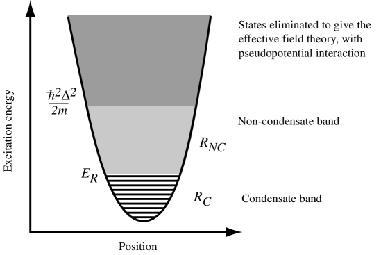
Figure 1: Schematic view of the condensate band, the non-condensate band, and eliminated states for a harmonic trap.

For the purposes of this paper we have to take into account two criteria:

• The highest energy states of the condensate band should have an occupation of the order of magnitude 5–10, so that we can apply Wigner function methods to all modes of the condensate band. In practice this means that

  $${k_{B}T\over E_{R}-\mu} \mathrel{\vbox{\hbox{$\sim$}\vskip-7.5pt\hbox{$>$} \vskip-1.0pt}} 5,$$ (12)

  since this corresponds to the high occupation limit of the Bose-Einstein distribution.

• The single particle energy levels of the noncondensate band should be essentially those of the trapping potential $V({\bf x})$, which is usually a harmonic potential. In [15] we showed that this is true to about 3%, provided that

  $$E_{R}/\mu_{C} \mathrel{\vbox{\hbox{$\sim$}\vskip-7.5pt\hbox{$>$} \vskip-1.0pt}} 3.$$ (13)

  The two criteria together lead to the requirement (assuming that the maximum value of $\mu_{C}\approx\mu$) that

  $$k_{B}T/\mu \mathrel{\vbox{\hbox{$\sim$}\vskip-7.5pt\hbox{$>$} \vskip-1.0pt}} 10,$$ (14)

  and this condition is usually satisfied in practice.

2.2.1 Definition of condensate band field operators

To effect the division between the two bands in the many-particle Hamiltonian we first note that the effective potential in the noncondensate band is considered to be little different from the trap potential. Thus we can expand $\psi({\bf x})$ in trap eigenfunctions, and define $\psi_{NC}({\bf x})$ to be that component which is expressible entirely in terms of eigenfunctions with energy eigenvalue larger than $E_{R}$. This means that $\phi({\bf x})$ is automatically defined through (11), and that it can be expressed in terms of trap eigenfunctions with energy eigenvalue less than $E_{R}$.

The division can be expressed in terms of projectors, whose form will be important in numerical implementations, as

$${\cal P}_{NC}({\bf x},{\bf x}^{\prime}) \equiv \sum_{E_{n}>E_{R}}Y_{n}^{*}({\bf x})Y_{n}({\bf x}^{\prime}),$$ (15)

$${\cal P}_{C}({\bf x},{\bf x}^{\prime}) \equiv 1-{\cal P}_{NC}({\bf x},{\bf x}^{\prime}).$$ (16)

Here the $Y_{n}({\bf x})$ are a complete set of trap eigenfunctions. Thus

$$\psi_{NC}({\bf x}) = \int d^{3}{\bf x}^{\prime}\,{\cal P}_{NC}({\bf x},{\bf x}^{\prime})\psi({\bf x}^{\prime})\equiv{\cal P}_{NC}\big{\{}\psi({\bf x})\big{\}},$$ (17)

$$\phi({\bf x}) = \int d^{3}{\bf x}^{\prime}\,{\cal P}_{C}({\bf x},{\bf x}^{\prime})\psi({\bf x}^{\prime})\,\,\,\,\equiv{\cal P}_{C}\big{\{}\psi({\bf x})\big{\}}.$$ (18)

2.2.2 Separation of condensate and non-condensate parts of the full Hamiltonian

The Hamiltonian is written in a form which separates it into three components; namely, those which act within $R_{NC}$ only, those which act within $R_{C}$ only, and those which cause transfers of energy or population between $R_{C}$ and $R_{NC}$. Thus we write

$$H=H_{NC}+H_{0}+H_{I,C},$$ (19)

in which $H_{NC}$ is the part of $H$ which depends only on $\psi_{NC}$, $H_{0}$ is the part which depends only on $\phi$, and that part of the interaction Hamiltonian which involves both condensate band and non-condensate band operators is called $H_{I,C}$. Substituting $\psi({\bf x})\to\phi({\bf x})+\psi_{NC}({\bf x})$ in the Hamiltonian, we get

$$H_{I,C}\equiv H^{(1)}_{I,C}+H^{(2)}_{I,C}+H^{(3)}_{I,C},$$ (20)

where the individual terms in $H_{I,C}$ are the terms involving operators from both bands, which cause transfer of energy and/or particles between $R_{C}$ and $R_{NC}$. We call the parts involving one $\phi$ operator

$$H^{(1)}_{I,C} \equiv u\int d^{3}{\bf x}\,\left(\psi_{NC}^{\dagger}({\bf x})\psi_{NC}^{\dagger}({\bf x})\psi_{NC}({\bf x})\right)\phi({\bf x})$$ (21)

$$+u\int d^{3}{\bf x}\,\phi^{\dagger}({\bf x})\left(\psi_{NC}^{\dagger}({\bf x})\psi_{NC}({\bf x})\psi_{NC}({\bf x})\right).$$

The parts involving two $\phi$ operators are called

$$H^{(2)}_{I,C} \equiv 2u\int d^{3}{\bf x}\,\psi_{NC}^{\dagger}({\bf x})\psi_{NC}({\bf x})\Big{(}\phi^{\dagger}({\bf x})\phi({\bf x})\Big{)}$$ (22)

$$+{u\over 2}\int d^{3}{\bf x}\,\psi_{NC}^{\dagger}({\bf x})\psi_{NC}^{\dagger}({\bf x})\Big{(}\phi({\bf x})\phi({\bf x})\Big{)}$$

$$+{u\over 2}\int d^{3}{\bf x}\,\psi_{NC}({\bf x})\psi_{NC}({\bf x})\Big{(}\phi^{\dagger}({\bf x})\phi^{\dagger}({\bf x})\Big{)}.$$

The parts involving three $\phi$ operators are called

$$H^{(3)}_{I,C} \equiv u\int d^{3}{\bf x}\,\Big{(}\phi^{\dagger}({\bf x})\phi^{\dagger}({\bf x})\phi({\bf x})\Big{)}\psi_{NC}({\bf x})$$ (23)

$$+u\int d^{3}{\bf x}\,\psi_{NC}^{\dagger}({\bf x})\Big{(}\phi^{\dagger}({\bf x})\phi({\bf x})\phi({\bf x})\Big{)}.$$

2.2.3 Connection to the notation of Davis et al.

Here we briefly make a link between the notation of this paper, which corresponds largely to that of the Quantum Kinetic Theory papers [14, 15, 16], and that of the finite temperature Gross-Pitaevskii equation papers [8, 9, 10].

• The condensate band $R_{NC}$ of Quantum Kinetic Theory roughly corresponds to the coherent region $C$ of the finite temperature Gross-Pitaevskii equation  papers, although there is the additional requirement in the latter that the mode occupations must be large. However, this is also a necessary condition for the condensate band in this paper.

• The non-condensate band $R_{NC}$ was called the incoherent region $I$ in finite temperature Gross-Pitaevskii equation papers.

• For the field operators we have the correspondences

  $$\phi({\bf x})\leftrightarrow\hat{\psi}(\mathbf{x}),\qquad\psi_{NC}({\bf x})\leftrightarrow\hat{\eta}(\mathbf{x}).$$ (24)

• The notations for the projectors are connected by

  $${\cal P}_{C}({\bf x},{\bf x}^{\prime})\leftrightarrow\hat{\mathcal{P}},\qquad{\cal P}_{NC}({\bf x},{\bf x}^{\prime})\leftrightarrow\hat{\mathcal{Q}}.$$ (25)

3 Derivation of the master equation

The description assumes that $R_{NC}$ is at least locally thermalized, and thus the atoms in these levels are treated simply as a heat bath and source of atoms for the levels in $R_{C}$. This is defined by requiring the field operator correlation functions to have a thermal form locally, and to have factorization properties like those which pertain in equilibrium. The precise nature of these local equilibrium requirements is specified in Sect. 3.2.3

3.1 Formal derivation of the master equation

The derivation of the master equation follows a rather standard methodology, formulated in [22], and as previously introduced in [14, 15, 16]. We project out the dependence on the non-condensate band by defining the condensate density operator as

$$\rho_{C} = {\rm Tr}_{NC}(\rho),$$ (26)

and a projector ${\cal P}$ on the space of density operators by

$${\cal P}\rho = \rho_{NC}\otimes{\rm Tr}_{NC}(\rho)\equiv\rho_{NC}\otimes\rho_{C},$$ (27)

and we also use the notation

$${\cal Q}\equiv 1-{\cal P}.$$ (28)

The equation of motion for the full density operator $\rho$ is the von Neumann equation

$$\dot{\rho} = -{i\over\hbar}[H_{NC}+H_{0}+H_{I},\rho],$$ (29)

$$\equiv ({\cal L}_{NC}+{\cal L}_{0}+{\cal L}_{I})\rho.$$ (30)

We use the Laplace transform notation for any function $f(t)$

$$\tilde{f}(s) = \int_{0}^{\infty}\rme^{-st}f(t)\,dt.$$ (31)

We then use standard methods to write the master equation for the Laplace transform of $v(t)\equiv{\cal P}\rho(t)$ as

$$s\tilde{v}(s)-v(0) = {\cal L}_{0}\tilde{v}(s)+{\cal P}{\cal L}_{I}\tilde{v}(s)+{\cal P}{\cal L}_{I}[s-{\cal L}_{NC}-{\cal L}_{0}-{\cal Q}{\cal L}_{I}]^{-1}{\cal Q}{\cal L}_{I}\tilde{v}(s).$$ (32)

In this form the master equation is basically exact. We shall make the approximation that the kernel of the second part, the $[\quad]^{-1}$ term, can be approximated by keeping only the terms which describe the basic Hamiltonians within $R_{C}$ or $R_{NC}$, namely the terms ${\cal L}_{NC}$ and ${\cal L}_{0}$. We then invert the Laplace transform, and make a Markov approximation to get

$$\dot{v}(t) = ({\cal L}_{0}+{\cal P}{\cal L}_{I})v(t)+\left\{{\cal P}{\cal L}_{I}\int_{0}^{t}d\tau\,\exp\left\{({\cal L}_{0}+{\cal L}_{I})\tau\right\}{\cal Q}{\cal L}_{I}\right\}v(t).$$ (33)

There are now a number of different terms to consider.

3.2 Terms in the master equation

3.2.1 Hamiltonian and forward scattering terms

These arise from the term $({\cal L}_{0}+{\cal P}{\cal L}_{I})v(t)$, and lead to a Hamiltonian term of the form

$$H_{C} \equiv H_{0}+H_{\rm forward},$$ (34)

where the forward scattering term is defined by

$$H_{\rm forward} \equiv 2u\!\int\!d^{3}{\bf x}\,\bar{n}_{NC}({\bf x})\phi^{\dagger}({\bf x})\phi({\bf x}),$$ (35)

where the non-condensate band particle density is

$$\bar{n}_{NC}({\bf x}) \equiv {\rm Tr}_{NC}\left\{\psi^{\dagger}_{NC}({\bf x)}\psi_{NC}({\bf x})\rho_{NC}\right\}.$$ (36)

This represents the condensate band Hamiltonian corrected for the effect of the average non-condensate density on the condensate. This correction is usually small, but can be included explicitly in our formulation of the master equation. The corresponding master equation term is

$$\left.\dot{\rho}_{C}\right|_{\rm Ham} \equiv -{\rmi\over\hbar}\left[H_{C},\rho_{C}\right].$$ (37)

3.2.2 Interaction between $R_{C}$ and $R_{NC}$

We now examine the terms in $H^{(1)}_{I}$, as defined in (21), which contain one $\phi({\bf x})$ or $\phi^{\dagger}({\bf x})$; explicitly, the term in Hamiltonian can be written

$$H^{(1)}_{I} = \int d^{3}{\bf x}\,Z_{3}({\bf x})\phi^{\dagger}({\bf x})+{\rm h.c.}$$ (38)

In this equation we have defined a notation

$$Z_{3}({\bf x}) = u\psi^{\dagger}_{NC}({\bf x})\psi_{NC}({\bf x})\psi_{NC}({\bf x}).$$ (39)

Substituting into the master equation (33), terms arise of which a typical one is of the form

$$-{1\over\hbar^{2}}\int d^{3}{\bf x}\int d^{3}{\bf x^{\prime}}\int_{-\infty}^{\,0}d\tau\,{\rm Tr}\left\{Z_{3}({\bf x})Z^{\dagger}_{3}({\bf x}^{\prime},\tau)\rho_{NC}\right\}\phi^{\dagger}({\bf x})\phi({\bf x^{\prime}},\tau)\rho_{C}(t).$$ (40)

Here we have introduced the notation for an arbitrary non-condensate band operator

$$A_{NC}({\bf x},t) = \rme^{\rmi H_{NC}t/\hbar}A_{NC}({\bf x})\rme^{-\rmi H_{NC}t/\hbar},$$ (41)

and for an arbitrary condensate band operator

$$B_{C}({\bf x},t) = \rme^{\rmi H_{C}t/\hbar}B_{C}({\bf x})\rme^{-\rmi H_{C}t/\hbar}.$$ (42)

This notation will be used frequently in the remainder of this section.

3.2.3 Correlation functions of $R_{NC}$

The terms involving $Z_{3},Z_{3}^{\dagger}$ are averaged over $\rho_{NC}$, which is assumed thermalized, and is therefore quantum Gaussian. This means that: i) We may make the replacement

$$\langle Z_{3}({\bf x})Z^{\dagger}_{3}({\bf x}^{\prime},\tau)\rangle \to 2\langle\psi_{NC}({\bf x})\psi^{\dagger}_{NC}({\bf x}^{\prime},\tau)\rangle\langle\psi_{NC}({\bf x})\psi^{\dagger}_{NC}({\bf x}^{\prime},\tau)\rangle\langle\psi^{\dagger}_{NC}({\bf x})\psi_{NC}({\bf x}^{\prime},\tau)\rangle.$$

(Terms involving $\langle\psi^{\dagger}_{NC}({\bf x})\psi_{NC}({\bf x}^{\prime})\rangle$ etc. do arise in principle, but give no contribution to the final result because of energy conservation considerations.)

ii) The time-dependence is needed only for small $\tau$, and in this case we can make appropriate replacements in terms of the one-particle Wigner function $F({\bf u},{\bf K})$

$$\left\langle\psi^{\dagger}_{NC}\left({\bf u}+{{\bf v}\over 2}\right)\psi_{NC}\left({\bf u}-{{\bf v}\over 2},\tau\right)\right\rangle \approx {1\over(2\pi)^{3}}\int_{R_{NC}}d^{3}{\bf K}\,F({\bf u},{\bf K})\rme^{-\rmi{\bf K}\cdot{\bf v}-\rmi\omega({\bf K},{\bf u})\tau},$$

$$\left\langle\psi_{NC}\left({\bf u}+{{\bf v}\over 2}\right)\psi^{\dagger}_{NC}\left({\bf u}-{{\bf v}\over 2},\tau\right)\right\rangle \approx {1\over(2\pi)^{3}}\int_{R_{NC}}d^{3}{\bf K}\,\left[F({\bf u},{\bf K})+1\right]\rme^{\rmi{\bf K}\cdot{\bf v}+\rmi\omega({\bf K},{\bf u})\tau},$$

where

$${\bf u} \equiv {{\bf x}+{\bf x}^{\prime}\over 2},$$ (46)

$${\bf v} \equiv {\bf x}-{{\bf x}^{\prime}},$$ (47)

$$\hbar\omega({\bf K},{\bf u}) = {\hbar^{2}{\bf K}^{2}\over 2m}+V({\bf u}).$$ (48)

Since the range of all the ${\bf K}$ integrals is restricted to $R_{NC}$, it is implicit that in all integrals $\hbar\omega({\bf K},{\bf u})>E_{R}$.

iii) This approximation is valid in the situation where $F({\bf K},{\bf u})$ is a smooth function of its arguments, and can be regarded as a local equilibrium assumption for particles moving in a potential which is comparatively slowly varying in space.

3.3 Growth terms

Using (3.2.3,3.2.3,3.2.3) we can now write

$$\langle Z_{3}({\bf x})Z^{\dagger}_{3}({\bf x}^{\prime},\tau)\rangle = {2u^{2}\over(2\pi)^{9}}\int\!\!\!\!\int\!\!\!\!\int\!d^{3}{\bf K}_{1}d^{3}{\bf K}_{2}d^{3}{\bf K}_{3}[1+F({\bf u},{\bf K}_{1})][1+F({\bf u},{\bf K}_{2})]F({\bf u},{\bf K}_{3})$$ (49)

$$\qquad\qquad\qquad\qquad\times\rme^{-\rmi(\omega_{1}+\omega_{2}-\omega_{3})\tau-\rmi({\bf K}_{1}+{\bf K}_{2}-{\bf K}_{3})\cdot{\bf v}},$$

where

$$\hbar\omega_{i} \equiv \hbar\omega({\bf K}_{i},{\bf u}).$$ (50)

3.3.1 Master equation terms for growth

We can write

$$\phi({\bf x},\tau) = \exp(-\rmi L_{C}\tau)\phi({\bf x}),$$ (51)

with

$$L_{C}\phi({\bf x}) \equiv -[H_{C},\phi({\bf x})]/\hbar.$$ (52)

This means that (40) can be written as

$$\int d^{3}{\bf u}\int d^{3}{\bf v}\,\phi^{\dagger}\left({\bf u}+{{\bf v}\over 2}\right)\left\{G^{(-)}({\bf u},{\bf v},L_{C})\phi\left({\bf u}-{{\bf v}\over 2}\right)\right\}\rho,$$ (53)

with

$$G^{(-)}({\bf u},{\bf v},\omega) = -{2u^{2}\over(2\pi)^{9}\hbar^{2}}\!\!\int\!\!\!\!\int\!\!\!\!\int\!d^{3}{\bf K}_{1}d^{3}{\bf K}_{2}d^{3}{\bf K}_{3}[1+F({\bf u},{\bf K}_{1})][1+F({\bf u},{\bf K}_{2})]F({\bf u},{\bf K}_{3})$$ (55)

$$\qquad\qquad\times\int_{-\infty}^{\,0}d\tau\,\rme^{\rmi(\omega_{1}+\omega_{2}-\omega_{3}-\omega)\tau-\rmi({\bf K}_{1}+{\bf K}_{2}-{\bf K}_{3})\cdot{\bf v}},$$

$$\approx -{u^{2}\over(2\pi)^{8}\hbar^{2}}\!\!\int\!\!\!\!\int\!\!\!\!\int\!d^{3}{\bf K}_{1}d^{3}{\bf K}_{2}d^{3}{\bf K}_{3}[1+F({\bf u},{\bf K}_{1})][1+F({\bf u},{\bf K}_{2})]F({\bf u},{\bf K}_{3})$$

$$\qquad\qquad\times\delta(\omega_{1}+\omega_{2}-\omega_{3}-\omega)\rme^{-\rmi({\bf K}_{1}+{\bf K}_{2}-{\bf K}_{3})\cdot{\bf v}}.$$

(The approximation made in (55) is to say $\int_{-\infty}^{\,0}d\tau\exp(-\rmi\Omega\tau)=\pi\delta(\Omega)+\rmi{\rm P}/\Omega\approx\pi\delta(\Omega)$, i.e., to neglect the principal value integral).

We will also need

$$G^{(+)}({\bf u},{\bf v},\omega) \approx -{u^{2}\over(2\pi)^{8}\hbar^{2}}\!\!\int\!\!\!\!\int\!\!\!\!\int\!d^{3}{\bf K}_{1}d^{3}{\bf K}_{2}d^{3}{\bf K}_{3}F({\bf u},{\bf K}_{1})F({\bf u},{\bf K}_{2})[1+F({\bf u},{\bf K}_{3})]$$ (56)

$$\qquad\qquad\times\delta(\omega_{1}+\omega_{2}-\omega_{3}-\omega)\rme^{-\rmi({\bf K}_{1}+{\bf K}_{2}-{\bf K}_{3})\cdot{\bf v}}.$$

If the noncondensate band is taken to be in thermal equilibrium

$$F({\bf u},{\bf K}) = {1\over\exp\left(\hbar\omega({\bf K},{\bf u})-\mu\over k_{B}T\right)-1},$$ (57)

there is the relation

$$G^{(+)}({\bf u},{\bf v},\omega) = \rme^{(\mu-\hbar\omega)/k_{B}T}G^{(-)}({\bf u},{\bf v},\omega).$$ (58)

This will still be true even if the equilibrium is merely local, with $\mu$ and $T$ depending on the position ${\bf u}$.

Collecting all relevant terms together, we get a master equation term in the form

$$\left.\dot{\rho}_{C}\right|_{\rm growth} = \int d^{3}{\bf u}\int d^{3}{\bf v}\left[\left\{G^{(-)}({\bf u},{\bf v},L_{C})\phi\left({\bf u}-{{\bf v}\over 2}\right)\right\}\rho_{C},\phi^{\dagger}\left({\bf u}+{{\bf v}\over 2}\right)\right]$$ (59)

$$-\int d^{3}{\bf u}\int d^{3}{\bf v}\left[\rho_{C}\left\{G^{(-)}({\bf u},{\bf v},L_{C})\phi^{\dagger}\left({\bf u}-{{\bf v}\over 2}\right)\right\},\phi\left({\bf u}+{{\bf v}\over 2}\right)\right]$$

$$+\int d^{3}{\bf u}\int d^{3}{\bf v}\left[\left\{G^{(+)}({\bf u},{\bf v},L_{C})\phi^{\dagger}\left({\bf u}-{{\bf v}\over 2}\right)\right\}\rho_{C},\phi\left({\bf u}+{{\bf v}\over 2}\right)\right]$$

$$-\int d^{3}{\bf u}\int d^{3}{\bf v}\left[\rho_{C}\left\{G^{(+)}({\bf u},{\bf v},L_{C})\phi\left({\bf u}-{{\bf v}\over 2}\right)\right\},\phi^{\dagger}\left({\bf u}+{{\bf v}\over 2}\right)\right].$$

3.4 Scattering terms

These come from terms involving two $\phi$ operators; of these terms, only those involving one $\phi$ and one $\phi^{\dagger}$ can yield a resonant term, corresponding to scattering of a non-condensate particle by the condensate. The effect of the non-resonant terms is neglected.

Thus we arrive at an approximation to $H^{(2)}_{I}$ in the form of a term

$$H^{(2)}_{I} \approx 2\int d^{3}{\bf x}\,Z_{2}({\bf x})U({\bf x})+{\rm h.c.},$$ (60)

where

$$Z_{2}({\bf x}) = u\psi_{NC}({\bf x})\psi_{NC}^{\dagger}({\bf x}),$$ (61)

$$U({\bf x}) \equiv \phi^{\dagger}({\bf x})\phi({\bf x}).$$ (62)

The term analogous to (40) in the master equation becomes, using the notation of (41,42),

$$-{4\over\hbar^{2}}\int_{-\infty}^{\,0}d\tau\,U({\bf x})U({\bf x}^{\prime},\tau)\int d^{3}{\bf x}\int d^{3}{\bf x^{\prime}}\langle Z_{2}({\bf x})Z^{\dagger}_{2}({\bf x^{\prime}},\tau)\rangle\rho_{C}(t).$$ (63)

3.4.1 Master equation terms for scattering

These arise from the term

$$\int d^{3}{\bf x}\int d^{3}{\bf x}^{\prime}\int_{-\infty}^{\,0}d\tau\,\,\left\langle\left[Z_{2}({\bf x})U({\bf x}),\left[Z_{2}({\bf x}^{\prime},\tau)U({\bf x}^{\prime},\tau),\rho\right]\right]\right\rangle_{\rm NC}.$$ (64)

We define

$$M({\bf u},{\bf v},\omega) = {2u^{2}\over(2\pi)^{5}\hbar^{2}}\int d^{3}{\bf K}_{1}\int d^{3}{\bf K}_{2}\,F({\bf K}_{1},{\bf u})[1+F({\bf K}_{2},{\bf u})]\rme^{\rmi({\bf K}_{1}-{\bf K}_{2})\cdot{\bf v}}$$ (65)

$$\qquad\qquad\times\delta(\omega_{1}-\omega_{2}-\omega),$$

and if $F({\bf K},{\bf u})$ corresponds to thermal equilibrium, as in (57), this satisfies the relation

$$M({\bf u},{\bf v},\omega) = \rme^{-\hbar\omega/k_{B}T}M({\bf u},{\bf v},-\omega).$$ (66)

The terms in the master equation arising from this part become

$$\left.\dot{\rho}_{C}\right|_{\rm scatt} = \int d^{3}{\bf u}\int d^{3}{\bf v}\left[U\left({\bf u}+{{\bf v}\over 2}\right),\left\{M({\bf u},{\bf v},L_{C})U\left({\bf u}-{{\bf v}\over 2}\right)\right\}\rho_{C}\right]$$ (67)

$$+\int d^{3}{\bf u}\int d^{3}{\bf v}\left[\rho_{C}\left\{M({\bf u},{\bf v},-L_{C})U\left({\bf u}-{{\bf v}\over 2}\right)\right\},U\left({\bf u}+{{\bf v}\over 2}\right)\right].$$

3.5 Terms involving three $\phi$ operators

The part of the interaction Hamiltonian can be written

$$H^{(3)}_{I} = u\int d^{3}{\bf x}\,\psi_{NC}({\bf x})\phi^{\dagger}({\bf x})\phi^{\dagger}({\bf x})\phi({\bf x})+{\rm h.c.}$$ (68)

The master equation term this time takes the form

$$-{u^{2}\over\hbar^{2}}\int_{-\infty}^{\,0}d\tau\int d^{3}{\bf x}\int d^{3}{\bf x^{\prime}}\,\phi^{\dagger}({\bf x}^{\prime},\tau)\phi({\bf x}^{\prime},\tau)\phi({\bf x}^{\prime},\tau)\phi^{\dagger}({\bf x})\phi^{\dagger}({\bf x})\phi({\bf x})$$

$$\qquad\qquad\qquad\qquad\qquad\qquad\times\langle\psi_{NC}({\bf x})\psi_{NC}^{\dagger}({\bf x^{\prime}})\rangle\rho_{C}(t).$$ (69)

These terms are probably very small, and will not be included in our analysis.

3.6 Connection with the finite temperature Gross-Pitaevskii equation of Davis et al.

The master equation terms described above are related to the terms in the finite temperature Gross-Pitaevskii equation, (29a-d) of  [8]. We have

Growth terms $$\longleftrightarrow U_{0}\hat{\mathcal{P}}\left\{\langle\hat{\eta}^{{\dagger}}({\bf x})\hat{\eta}({\bf x})\hat{\eta}({\bf x})\rangle\right\},$$

Scattering terms $$\longleftrightarrow U_{0}\hat{\mathcal{P}}\left\{2\psi({\bf x})\langle\hat{\eta}^{{\dagger}}({\bf x})\hat{\eta}({\bf x})\rangle\right\},$$

Terms with three $$\phi \longleftrightarrow U_{0}\hat{\mathcal{P}}\left\{2|\psi({\bf x})|^{2}\langle\hat{\eta}({\bf x})\rangle+\psi({\bf x})^{2}\langle\hat{\eta}^{{\dagger}}({\bf x})\rangle\right\}$$ operators

We point out that the finite temperature Gross-Pitaevskii equation scattering term also includes the forward scattering part of the Hamiltonian in (35) of this paper. The anomalous term of the FTGPE, analyzed in Sect. 5.2 of [8] is mainly responsible for the replacement of the true interatomic potential by the contact potential in the equations of motion, and hence the introduction of the momentum cutoff $\Delta$. In this paper, as noted in Sect. 2.2, we have already performed this spatial coarse-graining in the Hamiltonian with the cutoff $\Delta$, and so any anomalous terms will be very small.

3.7 The full master equation and its stationary solution

The full master equation can now be written

$$\dot{\rho}_{C} = \left.\dot{\rho}_{C}\right|_{\rm Ham}+\left.\dot{\rho}_{C}\right|_{\rm growth}+\left.\dot{\rho}_{C}\right|_{\rm scatt},$$ (70)

where the individual terms are given by (37), (59) and (67). The stationary solution of each of the terms in the master equation (70), and therefore of the master equation itself, is given by the grand canonical form

$$\rho_{\rm s} \propto \exp\left(\mu N_{C}-H_{C}\over k_{B}T\right).$$ (71)

This follows: i) From the equality of terms in (59) like

$$\left\{G^{(-)}({\bf u},{\bf v},L_{C})\phi\left({\bf u}-{{\bf v}\over 2}\right)\right\}\rho_{\rm s} = \rho_{\rm s}\left\{G^{(+)}({\bf u},{\bf v},L_{C})\phi\left({\bf u}-{{\bf v}\over 2}\right)\right\},$$ (72)

which can be derived using using (58), (71) and the commutation relation

$$[N_{C},\phi] = -\phi,$$ (73)

between the field operator and the condensate band number operator

$$N_{C} = \int d^{3}{\bf x}\,\phi^{\dagger}({\bf x})\phi({\bf x)}.$$ (74)

ii) From the equality of terms in (67) like

$$\left\{M({\bf u},{\bf v},L_{C})U\left({\bf u}-{{\bf v}\over 2}\right)\right\}\rho_{\rm s} = \rho_{\rm s}\left\{M({\bf u},{\bf v},-L_{C})U\left({\bf u}-{{\bf v}\over 2}\right)\right\}.$$ (75)

which can be derived using (66), (71) and the fact that $[U({\bf x}),N_{C}]=0$.

3.8 The projection into the condensate band

In exactly the same way as noted in Sect. 2.1, the projection into the condensate band means that the operator $L_{C}$ has a projected expression when it acts on the condensate band operator $\phi({\bf x})$

$$\rmi{L_{C}\phi({\bf x})} = {\cal P}_{C}\left\{-{\hbar^{2}\over 2m}\nabla^{2}\phi({\bf x})+V({\bf x})+u\phi^{\dagger}({\bf x})\phi({\bf x})\phi({\bf x})\right\},$$ (76)

which arises directly from the fact that the field operator commutation relation is

$$\left[\phi({\bf x}),\phi^{\dagger}({\bf x}^{\prime})\right] = {\cal P}_{C}({\bf x},{\bf x}^{\prime}).$$ (77)

The projector ${\cal P}_{C}({\bf x},{\bf x}^{\prime})$ will occur frequently in the remainder of this paper, as an expression of the fact that the field operator $\phi({\bf x})$ and any approximate representations of it must always be expressible in terms of the wavefunctions which span the condensate band.

This projector will play a significant rôle in the practical implementation of the master equations, and is by no means merely a formal requirement. It has two principal effects:

• The nonlocality generates a spatial smoothing function, and because the cutoff is in terms of energy rather than momentum, the smoothing is stronger where the potential $V({\bf x})$ is larger.

• At positions where $V({\bf x})>E_{R}$, all wavefunctions in the projector are exponentially small, so the projector is essentially zero. This means that the boundary conditions on any simulational grid are simply that any representation of $\phi({\bf x})$ is zero there.

Although the projector can be written down quite easily using (15), this expression is not computationally simple—efficient numerical implementation is essential for the practicality of any simulations.

4 Approximate forms of the master equation

It is not possible to contemplate a numerical solution of the master equation in the form given in (70), but there are two ways in which simplifications can be made, which we will call the “quantum optical” master equation and the “high temperature” master equation.

4.1 The “quantum optical” master equation for a Bose-Einstein condensate

The method chosen in [15]  was to expand the field operators in eigenoperators of $L_{C}$. Thus, one wrote

$$\phi({\bf x}) = \sum_{m}X_{m}({\bf x}),$$ (78)

where the eigenoperator requirement is (see [15], eq. (28))

$$L_{C}X_{m}({\bf x})=\epsilon_{m}X_{m}({\bf x}).$$ (79)

This method has two disadvantages

• We cannot calculate the operators $X_{m}({\bf x})$ exactly, although when the Bogoliubov approximation is valid, they can be expressed in terms of Bogoliubov amplitudes, as was done in [15].

• The resulting master equation (eq (50a–f) of [15]) can only be derived by making a rotating wave or random phase approximation, whose validity can be questioned. However, this master equation is of the Lindblad form ([22] Sect. 5.2.2), and this is a highly desirable, though not absolutely essential, property, since it guarantees that solutions are density operators with non-negative eigenvalues.

Useful results have been derived using this form of the master equation.

4.2 The “high temperature” master equation for a Bose-Einstein condensate

In this case the essential approximation relies on the fact that eigenfrequencies of $L_{C}$ are small compared to the temperature; precisely

$$\hbar|\epsilon_{m}|/k_{B}T \ll 1.$$ (80)

This is a condition which is very often met, to an accuracy of at least 10%, at temperatures which one would normally find in a degenerate Bose gases with a significant non-condensate fraction. In some sense, the nomenclature “high temperature” is misleading, but in a strict sense, it is a fair description of the kind of limit contemplated in (80). The master equation that can be derived is not of the Lindblad form, as indeed is also the case for the unapproximated master equation (70). However, as shown in [23], this probably only means that there are transient situations arising after unrealistic (although physically acceptable) initial conditions which give rise to a non-positive definite density operator. Such transients usually evolve on a time scale more rapid than that used to derive the master equation, so they have no physical significance.

We now develop the approximations based on the condition (80). The functions $G^{(\pm)}({\bf u},{\bf v},\omega)$ and $M({\bf u},{\bf v},\omega)$ can then be evaluated approximately for $\hbar\omega\ll k_{B}T$, the limit in which the stochastic Gross-Pitaevskii equation was originally derived [1]. Under this condition we can use (66) to give

$$M({\bf u},{\bf v},\omega) = \left(1-{\hbar\omega\over 2k_{B}T}\right)M({\bf u},{\bf v},0).$$ (81)

For $G^{(\pm)}({\bf u},{\bf v},\omega)$ we can take $G^{(+)}({\bf u},{\bf v},\omega)\approx G^{(+)}({\bf u},{\bf v},0)$ (Using for example the formula (153) of [15]) and then write using ( 58)

$$G^{(-)}({\bf u},{\bf v},\omega)\approx\left(1-{\mu-\hbar\omega\over k_{B}T}\right)G^{(+)}({\bf u},{\bf v},0).$$ (82)

These two expressions will be used to derive all that follows in this paper, but more accurate expressions could be used, involving higher powers of $\hbar\omega/k_{B}T$, which would extend the range of the approximation, as noted by Stoof [3, 24, 25]. The highest value of $\epsilon_{m}$ available is of the order of $E_{R}-\mu\approx 2\mu$, so that this method would be available for smaller chemical potentials and lower temperatures.

4.2.1 Growth terms

Both of $G^{(\pm)}$ are sharply peaked as functions of ${\bf v}$, so we will also approximate $\phi({\bf u}\pm{\bf v}/2)\approx\phi({\bf u})$ in the growth terms, and get the approximate master equation terms

$$\left.\dot{\rho}_{C}\right|_{\rm growth} = \left(1-{\mu\over k_{B}T}\right)\int d^{3}{\bf x}\,\bar{G}({\bf x})\left\{\left[\phi({\bf x})\rho_{C},\phi^{\dagger}({\bf x})\right]-\left[\rho_{C}\phi^{\dagger}({\bf x}),\phi({\bf x})\right]\right\}$$ (83)

$$+{\hbar\over k_{B}T}\int d^{3}{\bf x}\,\bar{G}({\bf x})\left\{\left[\left(L_{C}\phi({\bf x})\right)\rho_{C},\phi^{\dagger}({\bf x})\right]-\left[\rho_{C}\left(L_{C}\phi^{\dagger}({\bf x})\right),\phi({\bf x})\right]\right\}$$

$$+\int d^{3}{\bf x}\,\bar{G}({\bf x})\left\{\left[\phi^{\dagger}({\bf x})\rho_{C},\phi({\bf x})\right]-\left[\rho_{C}\phi({\bf x}),\phi^{\dagger}({\bf x})\right]\right\}.$$

Here we have used the notation

$$\bar{G}({\bf x}) \equiv \int d^{3}{\bf v}\,G^{(+)}({\bf x},{\bf v},0).$$ (84)

4.2.2 Scattering terms

We cannot make the approximation $\phi({\bf u}\pm{\bf v}/2)\approx\phi({\bf u})$ in the scattering terms, because $\int d^{3}{\bf v}\,M({\bf x},{\bf v},0)$ is ill defined, since it involves the product $\delta(\omega_{1}-\omega_{2})\delta({\bf K}_{1}-{\bf K_{2}})$. In this case we must keep the full dependence on ${\bf v}$:

$$\left.\dot{\rho}_{C}\right|_{\rm scatt} = -\int d^{3}{\bf x}d^{3}{\bf v}\,M({\bf x},{\bf v},0)\bigg{\{}\left[U({\bf x}+{\bf v}/2),[U({\bf x}-{\bf v}/2),\rho_{C}]\right]$$

$$\qquad\qquad\qquad\qquad+{\hbar\over 2k_{B}T}\left[U({\bf x}+{\bf v}/2),[\left(L_{C}U({\bf x}-{\bf v}/2)\right),\rho_{C}]_{+}\right]\bigg{\}}.$$

4.2.3 Estimate of the amplitude

To understand the nature of the scattering term, one can evaluate the Fourier transform

$$\tilde{M}({\bf x},{\bf k},0) \equiv {1\over(2\pi)^{3}}\int d^{3}{\bf v}\,\rme^{-\rmi{\bf k}\cdot{\bf v}}M({\bf x},{\bf v},0),$$ (86)

$$= {2u^{2}\over(2\pi)^{5}\hbar^{2}}\int d^{3}{\bf K}_{1}\int d^{3}{\bf K}_{2}\,F({\bf K}_{1},{\bf x})[1+F({\bf K}_{2},{\bf x})]\delta({\bf K}_{1}-{\bf K}_{2}-{\bf k})$$

$$\qquad\qquad\times\delta(\omega_{1}-\omega_{2}).$$

Since $F({\bf K},{\bf x})$ depends on

$$e_{\bf K}({\bf x}) \equiv {\hbar^{2}{\bf K}^{2}\over 2m}+V({\bf x})\equiv\hbar\omega({\bf K},{\bf x}),$$ (87)

this can be written as

$$\tilde{M}({\bf x},{\bf k},0) = {2u^{2}\over(2\pi)^{5}\hbar^{2}}\int d^{3}{\bf K}\,F(e_{\bf K},{\bf x})[1+F(e_{\bf K},{\bf x})]{2m\over\hbar}\delta(2{\bf K}\cdot{\bf k}-{\bf k}^{2}).$$ (88)

We can choose the $x$-axis in the ${\bf K}$-integration parallel to ${\bf k}$ and and use the delta function to eliminate $K_{x}\to|{\bf k}|/2$. Using the notation $\hat{\bf K}\equiv(K_{y},K_{z})$, so that

$$e_{\bf K}({\bf x}) \to \hat{e}_{\hat{\bf K}}({\bf k},{\bf x})\equiv{\hbar^{2}(\hat{\bf K}^{2}+|{\bf k}|^{2}/4)\over 2m}+V({\bf x}),$$ (89)

we can write

$$\tilde{M}({\bf x},{\bf k},0) = {2mu^{2}\over(2\pi)^{5}\hbar^{3}|{\bf k}|}\int d^{2}\hat{\bf K}\,f_{T,\mu}\left(\hat{e}_{\hat{\bf K}}({\bf k},{\bf x})\right)\left\{1+f_{T,\mu}\left(\hat{e}_{\hat{\bf K}}({\bf k},{\bf x})\right)\right\},$$ (90)

where

$$f_{T,\mu}(y) \equiv 1\over{\rme^{(y-\mu)/k_{B}T}-1}.$$ (91)

Using (89), we can change the integration variable to $\hat{e}_{\hat{\bf K}}({\bf k},{\bf x})$, where the lower limit of the integration is now

$$E_{\rm min}({\bf k},{\bf x}) \equiv \max\left(E_{R},V({\bf x})+\hbar^{2}|{\bf k}|^{2}/8m\right)/k_{B}T.$$ (92)

The integral then can be written

$$\tilde{M}({\bf x},{\bf k},0) = {2mu^{2}\over(2\pi)^{5}\hbar^{3}|{\bf k}|}{2\pi mk_{b}T\over\hbar^{2}}\int_{(E_{\rm min}-\mu)/k_{B}T}^{\infty}{\exp(y)\,dy\over[\exp(y)-1]^{2}},$$ (93)

$$= {2mu^{2}\over(2\pi)^{5}\hbar^{3}|{\bf k}|}{2\pi mk_{b}T\over\hbar^{2}}{1\over\exp\big{(}({E_{\rm min}({\bf k},{\bf x})}-\mu)/k_{B}T\big{)}-1},$$ (94)

$$\approx {8a^{2}(k_{B}T)^{2}\over(2\pi)^{2}\hbar({E_{\rm min}({\bf k},{\bf x})}-\mu)|{\bf k}|}.$$ (95)

The principal dependence on ${\bf k}$ comes from the $1/|{\bf k}|$ term, which is most significant for small $|{\bf k}|$. The operators $U({\bf x}\pm{\bf v}/2)$ are restricted to the condensate band, and thus will be significant only for ${\bf x}$ such that $E_{R}>V({\bf x})$. Thus the major contribution comes from situations such that $E_{\rm min}({\bf k},{\bf x})=E_{R}$, in which case the only ${\bf k}$ dependence comes from the $1/|{\bf k}|$ term, and we can write

$$\tilde{M}({\bf x},{\bf k},0) \to {{\cal M}\over(2\pi)^{3}|{\bf k}|},$$ (96)

where we define

$${\cal M} \equiv {8a^{2}(k_{B}T)^{2}\over(2\pi)^{2}\hbar({E_{R}}-\mu)}.$$ (97)

4.2.4 Approximate local form

The form (95) is nonlocal, and this may be an important feature. Nevertheless, we can try to write an approximate local equivalent in the form (which is essentially of the form of the quantum Brownian motion master equation as described in [22] Sect. 3.6.1)

$$\left.\dot{\rho}_{C}\right|_{\rm scatt} = -\int d^{3}{\bf x}\,\bar{M}({\bf x})\bigg{\{}\left[U({\bf x}),[U({\bf x}),\rho_{C}]\right]+{\hbar\over 2k_{B}T}\left[U({\bf x}),[\left(L_{C}U({\bf x})\right),\rho_{C}]_{+}\right]\bigg{\}}.$$

However, the correct choice of $\bar{M}({\bf x})$ is not straightforward; a possible estimate can be made by taking ${\bf k}={\bf k}_{1}-{\bf k}_{2}$, where $\hbar{\bf k}_{i}$ are the momenta of two particles in the condensate band. We then compute the average of (95) over the region $R_{C}$ such that $|{\bf k}_{1,2}|\leq\sqrt{2m\big{(}E_{R}-V({\bf x})\big{)}}/\hbar$, on the assumption of a noninteracting excitation spectrum:

$$\left.{1\over|{\bf k}_{1}-{\bf k}_{2}|}\right|_{\rm av} \equiv \int_{R_{C}}{d^{3}{\bf k}_{1}d^{3}{\bf k}_{2}\over|{\bf k}_{1}-{\bf k}_{2}|}\bigg{/}\int_{R_{C}}d^{3}{\bf k}_{1}d^{3}{\bf k}_{2},$$ (99)

$$= {6\hbar\,\Theta\big{(}{E_{R}-V({\bf x})}\big{)}\over 5\sqrt{2m\big{(}E_{R}-V({\bf x})\big{)}}}.$$ (100)

The singularity when $E_{R}=V({\bf x})$ is harmless, since the occupation is also zero there. Thus we can choose

$$\bar{M}({\bf x}) = {16\pi a^{2}(k_{B}T)^{2}\over\hbar({E_{R}}-\mu)}\left.{1\over|{\bf k}_{1}-{\bf k}_{2}|}\right|_{\rm av}.$$ (101)

4.2.5 Comparison of local and full forms

There are obvious technical advantages in using the local form (4.2.4) of the scattering term instead of the full form (4.2.2). The local form will give the correct stationary distribution for any choice of $\bar{M}({\bf x})$, and is in at least this sense acceptable. The main difference is that the local form gives essentially the same scattering rate at all momentum transfers, whereas the full form gives a significant drop off at high momentum transfers, and this is known to be a significant feature of the kinetics when this is treated by forms of the quantum Boltzmann equation, as noted for example in the papers of Svistunov, Kagan and Shlyapnikov [26, 27], the idea of “flux” in energy space is used, based on the locality in energy space of the collision integral.

5 Wigner function representation

5.1 Fokker-Planck equations

Fokker-Planck equations can be derived by using the transforms of [22], as described in [1]. None of the three principal terms (Hamiltonian, growth, scattering) can be put exactly in the form of a genuine probabilistic Fokker-Planck equation, but on the assumption that higher order derivatives become less significant, an approximate probabilistic Fokker-Planck, valid for large occupations, can be derived.

The methodology used can be demonstrated for one part of $\left.\rho_{C}\right|_{\rm growth}$:

$$\int d^{3}{\bf x}\,\bar{G}({\bf x})\left[\left[\phi({\bf x}),\rho_{C}\right]-{1\over k_{B}T}\{\mu\phi({\bf x})-\hbar{\bar{L}_{C}}\phi({\bf x})\}\rho_{C}\,,\,\phi^{\dagger}({\bf x})\right].$$ (102)

The transformation to a Fokker-Planck equation for the Wigner function $W$ of the phase space field function $\alpha({\bf x})$ is achieved by the mappings:

$$[\rho_{C},\phi^{\dagger}({\bf x})] \,\to\, {\bar{\delta}W\over\bar{\delta}\alpha^{*}({\bf x})},$$ (103)

$$[\phi({\bf x}),\rho_{C}] \to {\bar{\delta}W\over\bar{\delta}\alpha({\bf x})},$$ (104)

$$\mu\phi({\bf x})\rho_{C} \to \mu\alpha({\bf x})W,$$ (105)

$$\hbar{L_{C}}\phi({\bf x})\rho_{C} \,\to\, \bar{L}_{C}\alpha({\bf x})W.$$ (106)

In this equation there are some important points of notation and approximation

• The fact that the condensate band is spanned by the finite set of wavefunctions $Y_{n}({\bf x})$—see (15)—means that we define the phase space amplitude by

  $$\alpha({\bf x}) \equiv \sum_{n}Y_{n}({\bf x})\alpha_{n},$$ (107)

  (where $\alpha_{n}$ are independent mode amplitudes) and that we define a modified functional differentiation operator

  $${\bar{\delta}\over\bar{\delta}\alpha({\bf x})} \equiv \sum_{n}Y^{*}_{n}({\bf x}){\partial\over\partial\alpha_{n}}.$$ (108)

  This would be a genuine functional differentiation operator if the full set of modes $Y_{n}({\bf x})$ were used instead of only the set within the condensate band. Notice that from these definitions

  $${\bar{\delta}\alpha({\bf x})\over\bar{\delta}\alpha({\bf x}^{\prime})} \equiv {\cal P}_{C}({\bf x},{\bf x}^{\prime}),$$ (109)

  whereas the right hand side is a delta function for a true functional differentiation operator.

• Including the effect of the mean field arising from the the non-condensate as an effective potential

  $$V_{\rm eff}({\bf x}) \equiv V({\bf x})+2u\bar{n}_{NC}({\bf x}),$$ (110)

  the projected Gross-Pitaevskii operator is introduced as

  $$\bar{L}_{C}\alpha({\bf x}) \equiv {\cal P}_{C}\left\{-{\hbar^{2}\nabla^{2}\alpha({\bf x})\over 2m}+V_{\rm eff}({\bf x})\alpha({\bf x})+u|\alpha({\bf x})|^{2}\alpha({\bf x})\right\}.$$ (111)

  The projector arises as a consequence of (103,104,109) etc.

• The two replacements (105,106) are approximate, not only in the sense that higher order derivatives are neglected, but also in the sense that all derivatives which should arise from the left hand side are neglected. This is not an essential aspect of the method, since we can technically still handle the first order derivative terms which would turn up in the right hand sides of (105,106), and these would produce only second order derivatives in the final Fokker-Planck equation. This would produce a fractional correction of order $\mu/k_{B}T$ to the noise terms only.

The projected Gross-Pitaevskii operator can be written in terms of the Gross-Pitaevskii Hamiltonian

$$H_{\rm GP} \equiv \int d^{3}{\bf x}\,\left\{{\hbar^{2}|\nabla\alpha({\bf x})|^{2}\over 2m}+V_{\rm eff}({\bf x})|\alpha({\bf x})|^{2}+{u\over 2}|\alpha({\bf x})|^{4}\right\},$$ (112)

in the form

$$\bar{L}_{C}\alpha({\bf x}) = {\bar{\delta}H_{\rm GP}\over\bar{\delta}\alpha^{*}({\bf x})}.$$ (113)

We also define the Gross-Pitaevskii particle number

$$N_{\rm GP} \equiv \int d^{3}{\bf x}\,|\alpha({\bf x})|^{2}.$$ (114)

The term (102) then transforms to the term in the Fokker-Planck equation

$$\int d^{3}{\bf x}\,\bar{G}({\bf x}){\bar{\delta}\over\bar{\delta}\alpha({\bf x})}\left\{{\bar{\delta}W\over\bar{\delta}\alpha^{*}({\bf x})}-{W\over k_{B}T}{\bar{\delta}(\mu N_{\rm GP}-H_{\rm GP})\over\bar{\delta}\alpha^{*}({\bf x})}\right\}.$$ (115)

Using the same kind of approximations, the scattering term (4.2.4) can be transformed to a corresponding form, and we obtain, putting all terms together, the Fokker-Planck equation

$${\partial W\over\partial t} = \int d^{3}{\bf x}\,{\bar{\delta}\over\bar{\delta}\alpha({\bf x})}\bigg{\{}{\rmi W\over\hbar}{\bar{\delta}H_{\rm GP}\over\bar{\delta}\alpha^{*}({\bf x})}+\bar{G}({\bf x})\left[{\bar{\delta}W\over\bar{\delta}\alpha^{*}({\bf x})}-{W\over k_{B}T}{\bar{\delta}(\mu N_{\rm GP}-H_{\rm GP})\over\bar{\delta}\alpha^{*}({\bf x})}\right]\bigg{\}}$$

$$-\int d^{3}{\bf x}\,{\bar{\delta}\over\bar{\delta}\alpha^{*}({\bf x})}\bigg{\{}{\rmi W\over\hbar}{\bar{\delta}H_{\rm GP}\over\bar{\delta}\alpha({\bf x})}-\bar{G}({\bf x})\left[{\bar{\delta}W\over\bar{\delta}\alpha({\bf x})}-{W\over k_{B}T}{\bar{\delta}(\mu N_{\rm GP}-H_{\rm GP})\over\bar{\delta}\alpha({\bf x})}\right]\bigg{\}}$$

$$+\int d^{3}{\bf x}\,d^{3}{\bf x}^{\prime}\,M\left({{\bf x}+{\bf x}^{\prime}\over 2},{\bf x}-{\bf x}^{\prime},0\right)\left[{\alpha^{*}({\bf x}){\bar{\delta}\over\bar{\delta}\alpha^{*}({\bf x})}-\alpha({\bf x}){\bar{\delta}\over\bar{\delta}\alpha({\bf x})}}\right]$$

$$\times\Bigg{\{}\alpha^{*}({\bf x}^{\prime})\left[{\bar{\delta}W\over\bar{\delta}\alpha^{*}({\bf x}^{\prime})}+{W\over k_{B}T}{\bar{\delta}H_{\rm GP}\over\bar{\delta}\alpha^{*}({\bf x}^{\prime})}\right]-\alpha({\bf x}^{\prime})\left[{\bar{\delta}W\over\bar{\delta}\alpha({\bf x}^{\prime})}+{W\over k_{B}T}{\bar{\delta}H_{\rm GP}\over\bar{\delta}\alpha({\bf x}^{\prime})}\right]\Bigg{\}}.$$

5.2 Stationary solutions of the Fokker-Planck equation

Independently of the forms of $\bar{G}({\bf x})$ and $M({\bf x},{\bf x}^{\prime})$, the stationary solution of the Fokker-Planck (5.1) equation is given by

$$W_{\rm s} \propto \exp\left({\mu N_{\rm GP}-H_{\rm GP}\over k_{B}T}\right).$$ (117)

This is the grand canonical distribution expected for a classical field theory whose field $\alpha({\bf x},t)$ obeys the Gross-Pitaevskii equation.

5.3 Stochastic Gross-Pitaevskii equations

The Fokker-Planck equation (5.1) is equivalent to a set of stochastic differential equations, which we shall write in the Stratonovich form, in a choice of forms in which various degrees of simplification are made of the scattering terms, as follows. The notation $\mathbf{(S)}$ to the right of an equation indicates that it is in Stratonovich form as in [28].

5.3.1 Full form of the stochastic differential equations

Using the full form of the scattering term, we have

$${\bf(S)}\,\,d\alpha({\bf x},t) = -{\rmi\over\hbar}\bar{L}_{C}\alpha({\bf x},t)\,dt$$ (118)

$$+{\cal P}_{C}\Bigg{\{}{\bar{G}({\bf x})\over k_{B}T}\left\{\mu\alpha({\bf x},t)-\bar{L}_{C}\alpha({\bf x},t)\right\}\,dt+dW_{G}({\bf x},t)$$

$$-{1\over 2k_{B}T}\int d^{3}{\bf x}^{\prime}M\left({{\bf x}+{\bf x}^{\prime}\over 2},{\bf x}-{\bf x}^{\prime},0\right)\alpha({\bf x})$$

$$\times\left\{\alpha^{*}({\bf x}^{\prime},t)\left(\bar{L}_{C}\alpha({\bf x}^{\prime},t)\right)-\alpha({\bf x}^{\prime},t)\left(\bar{L}_{C}\alpha({\bf x}^{\prime},t)\right)^{*}\right\}\,dt$$

$$\qquad\qquad\qquad\qquad\qquad\qquad\qquad+\rmi\alpha({\bf x})\,dW_{M}({\bf x},t)\Bigg{\}}.$$

The noise $dW_{G}({\bf x},t)$ is complex, while $dW_{M}({\bf x},t)$ is real; they are independent of each other, and satisfy the relations

$$dW^{*}_{G}({\bf x},t)dW_{G}({\bf x}^{\prime},t) = 2\bar{G}({\bf x})\delta({\bf x}-{\bf x}^{\prime})\,dt,$$ (119)

$$dW_{G}({\bf x},t)dW_{G}({\bf x}^{\prime},t) = dW^{*}_{G}({\bf x},t)dW^{*}_{G}({\bf x}^{\prime},t)=0,$$ (120)

$$dW_{M}\left({\bf x},t\right)dW_{M}\left({\bf x}^{\prime},t\right) = 2M\left({{\bf x}+{\bf x}^{\prime}\over 2},{\bf x}-{\bf x}^{\prime},0\right)\,dt.$$ (121)

5.3.2 Simplified non-local form

The implementation of the last two lines of (118) obviously presents some technical issues. However, if we simplify (95) by setting $E_{\rm min}({\bf k},{\bf x})\to E_{R}$ (as discussed there), the nonlocal form can be considerably simplified. The operator $1/\sqrt{-\nabla^{2}}$, of which $1/|{\bf k}|$ is the Fourier transform, is not singular when acting on functions with well behaved Fourier transform as ${\bf k}\to 0$. Using this, the stochastic differential equation becomes

$${\bf(S)}\,\,d\alpha({\bf x},t) = -{\rmi\over\hbar}\bar{L}_{C}\alpha({\bf x},t)\,dt$$ (122)

$$+{\cal P}_{C}\Bigg{\{}{\bar{G}({\bf x})\over k_{B}T}\left\{\mu\alpha({\bf x},t)-\hbar{\bar{L}_{C}}{\alpha({\bf x},t)}\right\}\,dt+dW_{G}({\bf x},t)$$

$$-{{\cal M\alpha({\bf x})}\over 2k_{B}T}{1\over\sqrt{-\nabla^{2}}}\left\{\alpha^{*}({\bf x},t)\bar{L}_{C}\alpha({\bf x},t)-\alpha({\bf x},t)\left(\bar{L}_{C}\alpha({\bf x},t)\right)^{*}\right\}\,dt$$

$$\qquad\qquad\qquad\qquad\qquad\qquad\qquad+\rmi\alpha({\bf x})\,dW_{\cal M}({\bf x},t)\Bigg{\}}.$$

The noise $dW_{G}({\bf x},t)$ is complex, while $dW_{\cal M}({\bf x},t)$ is real; they are independent of each other, and satisfy the relations

$$dW^{*}_{G}({\bf x},t)dW_{G}({\bf x}^{\prime},t) = 2\bar{G}({\bf x})\delta({\bf x}-{\bf x}^{\prime})\,dt,$$ (123)

$$dW_{G}({\bf x},t)dW_{G}({\bf x}^{\prime},t) = dW^{*}_{G}({\bf x},t)dW^{*}_{G}({\bf x}^{\prime},t)=0,$$ (124)

$$dW_{\cal M}({\bf x},t)dW_{\cal M}({\bf x}^{\prime},t) = {2{\cal M}\over\sqrt{-\nabla^{2}}}\delta({\bf x}-{\bf x}^{\prime})\,dt.$$ (125)

5.3.3 Local form of the stochastic differential equations

These take the form

$${\bf(S)}\,\,d\alpha({\bf x},t) = -{\rmi\over\hbar}\bar{L}_{C}\big{(}\alpha({\bf x},t)\big{)}\,dt$$ (126)

$$+{\cal P}_{C}\Bigg{\{}{\bar{G}({\bf x})\over k_{B}T}\left\{\mu\alpha({\bf x},t)-\hbar{\bar{L}_{C}}{\alpha({\bf x},t)}\right\}\,dt+dW_{G}({\bf x},t)$$

$$-{\bar{M}({\bf x})\alpha({\bf x})\over 2k_{B}T}\left\{\alpha^{*}({\bf x},t)\bar{L}_{C}\alpha({\bf x},t)-\alpha({\bf x},t)\left(\bar{L}_{C}\alpha({\bf x},t)\right)^{*}\right\}\,dt$$

$$\qquad\qquad\qquad\qquad\qquad\qquad\qquad+\rmi\alpha({\bf x})\,dW_{\bar{M}}({\bf x},t)\Bigg{\}}.$$

The noise $dW_{G}({\bf x},t)$ is complex, while $dW_{\bar{M}}({\bf x},t)$ is real; they are independent of each other, and satisfy the relations

$$dW^{*}_{G}({\bf x},t)\,dW_{G}({\bf x}^{\prime},t) = 2\bar{G}({\bf x})\,\delta({\bf x}-{\bf x}^{\prime})\,dt,$$ (127)

$$dW_{G}({\bf x},t)\,dW_{G}({\bf x}^{\prime},t) = dW^{*}_{G}({\bf x},t)\,dW^{*}_{G}({\bf x}^{\prime},t)=0,$$ (128)

$$dW_{\bar{M}}({\bf x},t)\,dW_{\bar{M}}({\bf x}^{\prime},t) = 2\bar{M}({\bf x})\,\delta({\bf x}-{\bf x}^{\prime})\,dt.$$ (129)

5.4 Comparison with other methods

The stochastic differential equations we have derived have similarities with those we have previously derived, as well as with Stoof’s. However, our way of implementing the idea of eliminating higher energy thermalized modes has significant differences from Stoof’s:

i) There are major technical differences in how the elimination is done. Ours is based on the ideas of quantum optics, which are used to develop a quantum mechanical master equation. The master equation is then transformed using the Wigner function to give a Fokker-Planck equation, which is equivalent to a stochastic differential equation. Stoof uses a functional integral formulation of the Keldysh method, in which the elimination is achieved in the action integral. This method is almost certainly equivalent to our quantum optical method. Thus, although the technical methods used appear very different, this is not physically significant.

ii) However the choice of what to eliminate is different. Stoof eliminates modes with energy $\mathrel{\vbox{\hbox{$\sim$}\vskip-7.5pt\hbox{$>$} \vskip-1.0pt}}\mu$, and finds a Fokker-Planck equation (equivalent to a stochastic differential equation) which involves self energy functions, which he evaluates using the many-body T-matrix method. In contrast we carry out the elimination as a two-stage process, as detailed in Sects. 2,3. Thus we separate the elimination process which is required to give an effective field theory from that required to give a master equation for the condensate band. This has the advantage that we do not need to use a many body T-matrix description.

iii) The equations which arise are given above as (118,122,126), depending on degrees of approximation used. The principal differences are the appearance of the projector, and the inclusion of scattering terms. There is also the implicit difference that the field variable we use is not exactly the same as Stoof’s, since it includes a wider range of states.

iv) Our earlier work [1] included the scattering terms, but was unable to give any precise value to them because of the crudeness of the methods used, and also for reasons related to the fact, which we have found in this paper, that the scattering cannot be described locally without making very crude approximations, such as those which lead to the form (126). The explicit appearance of the projector in the equations did not occur there or in Stoof’s method. It is possible that in numerical implementation, the projector will not always be essential, but we are confident that there are situations in which its inclusion will be important.

6 Conclusions and outlook

The problem we have set ourselves in this paper is to produce a description of finite temperature condensed or nearly condensed Bose gases which is both accurate and implementable. Apart from those used to derive the basic Markovian master equation (33), there are only two significant approximations made in our derivation:

• The energy eigenvalues of the excitations are small compared to temperature, as noted in Sect. 4.2. This is needed to get a master equation of a reasonably simple kind, the “high temperature master equation.”

• The occupations of the modes being treated in the condensate band are significantly larger than unity, as noted in Sect. 5.1. This is essential to be able to use a Wigner function representation of the master equation which becomes equivalent to a classical field representation.

These two conditions are essentially the same, since the occupation of a mode of energy $\epsilon$ is large if $\epsilon\ll k_{B}T$, even though the reasons for the conditions are quite independent. Therefore, it is clear that if one is using the “high temperature master equation,” then it is also sensible to use the Wigner function classical field representation, since the two are accurate to the same degree of approximation.

6.1 The validity of the classical field representation

Classical field representations have often been introduced heuristically by the argument that the quantum field operator can be replaced by a classic field function provided the occupations of the modes are high. The Wigner function methodology which we use gives systematic way of implementing these heuristic ideas, and gives a way a assessing the validity of the formalism. It is important to realize that, when formulated through the Wigner function, the classical field method gives a truly quantum mechanical description of the system, subject only to the technical approximations made. This means that we expect the major quantum mechanical aspects to be correctly treated; in other words, the classical field method, correctly and carefully formulated, has no heuristic approximations introduced to provide refuge from quantum mechanics—it is a valid way of treating quantum mechanics in a certain degree of approximation, which fortunately behaves very much like a classical description.

As a result, certain quantum properties make their presence felt when using this method. The Wigner function exhibits “vacuum occupation” of the modes—the mean square of the classical field is non-zero even when there are no particles. This follows from the relationship between the classical field averages and the quantum averages in the form

$$\left\langle a^{\dagger}a+aa^{\dagger}\over 2\right\rangle = \int d^{2}\alpha\,|\alpha|^{2}W(\alpha,\alpha^{*}),$$ (130)

which says that the minimum occupation exhibited by the classical field is the “vacuum occupation,” half a particle per mode—an expression of the Heisenberg uncertainty principle. When summed over the infinite number of modes which constitute the full system, this gives a divergent field function; thus a cutoff must be introduced, such as the one we have chosen, which defines the boundary of the condensate band.

There are two different ways in which the classical field method applied to the condensate band can be valid.

• The temperature may be so low that there is little occupation at the top of the condensate band, so that all of the noise terms derived in Sect. 5 are zero. At low energies, the excitations of a Bose condensate are largely phonon-like, and amount to quantized shape and density oscillations of the condensate itself. These are only noticeable if their occupation is large; modes with low occupation, although badly described by the classical field method, provide a completely negligible contribution to the system.

  However, since there is no external noise, in this case the initial occupations of the modes must be chosen so as to represent the existence of a finite temperature. Even if the temperature is zero, these occupations must be chosen to give the correct “vacuum occupation,” and this gives rise to irreversible effects, as first noted by Steel et al. [29].

• If the temperature is not very low, the total number of particle in modes with occupations $\mathrel{\vbox{\hbox{$\sim$}\vskip-7.5pt\hbox{$<$} \vskip-1.0pt}}1$ can be very significant, and this is necessarily the case during the process of condensate growth from a vapour. The influence of these modes has to be included, and this is what has been done in this paper.

  In principle the initial conditions should be chosen as in i) to give the right “vacuum occupation”, but their effect rapidly dies out because of the irreversible coupling to the reservoir which generates the noise and damping terms.

6.2 The degenerate non-condensed Bose gas

It is known that during the process of condensate growth the occupations of a large number of modes become significantly larger than one before the appearance of a single dominant mode, the condensate. These modes are of course describable by our stochastic classical field equations (118–129), since we have nowhere assumed the existence of a condensate, and because their high occupation makes the classical field method valid. Kagan, Svistunov and Shlyapnikov [27] in their pioneering work on the initiation of Bose-Einstein condensation, also argued that a description in terms of the Gross-Pitaevskii equation was possible for such a system. However, because their philosophy was more qualitative, the technical details which we are compelled to attend to do not appear in their work.

6.3 The projector into the condensate band

One of the essential features of the description is the presence of a projector in the equations of motion for the classical field. This prevents non-condensate band modes being wrongly included in numerical simulations. Such a projector has already been implemented in [8, 9, 10], but only for a homogeneous system. While the projector for a system with a trap potential can be written down explicitly as in (15-16), it is not an easy task to implement this projector efficiently.

The projector deals correctly with two problems which arise in practical simulations:

• The fineness of the mesh: The distance between mesh points determines the highest momentum which can be represented in the simulation. However, one cannot choose this to be the physical cutoff, even in the case of no trapping potential, since nonlinear terms such as ${\cal P}_{C}\left\{|\alpha({\bf x})|^{2}\alpha({\bf x})\right\}$ in (111) are wrongly represented this way. To represent this term correctly without aliasing, the numerical wavenumber cutoff must extend to at least two times the physical cutoff. If one assumes the physical cutoff is to be given by the mesh fineness, incorrect results will be obtained unless there is no significant occupation above one half of the mesh wavenumber cutoff.

  In addition, when a trap potential is present, a cut at a minimum wavelength does not correspond to a cut at definite energy. This would mean that even non-interacting atoms would pass from the condensate band to the non-condensate band with the progression of time, presenting some difficulties for the formalism

• The boundary condition at the edge of the spatial grid: Because the projector involves trap eigenfunctions only up to energy $E_{R}$, in the case of a non-vanishing trap potential there is a distance $R$ such that for $|{\bf x}|>R$ projected functions become exponentially small. This means that not only are the field functions $\alpha({\bf x})$ of Sect. 5 exponentially small there, but also the added noise terms as well. Therefore in practical simulations on a grid of finite size, the issue of the boundary condition for the noise and the field function at the edge of the grid is determined; the simulation region must be so large that all field and noise functions can be set equal to zero at the boundary.

  Where there is no trap potential, the box inside which the simulation is being implemented has real physical significance, and periodic boundary conditions are usually chosen.

6.4 Applications

• Condensate growth: The theory of condensate growth is at this stage not entirely satisfactory—there is still disagreement between theory and experiment under certain conditions [30, 31]. The main defect in computations of condensate growth [30, 31, 32, 33, 34, 35, 36] to date is an inadequate treatment of the phonon-like quasiparticle excitations. Using the formulation proposed here would definitely include these correctly.

• Vortex lattice growth: The theoretical situation in the growth of vortex lattices is in a very preliminary stage. The stabilization of the vortices into a lattice is clearly a result of some kind of irreversible process, for which a phenomenological model was first proposed by Tsubota et al. [37], while we presented a physically based model [38] based on a rotating frame version of our phenomenological growth equation [1] which attributed the necessary irreversibility to interaction with a thermal cloud.

  In contrast, Lobo et al. [39] used a simple stochastic classical field model of the type mentioned above, in which the noise arises from initial conditions with no interaction with a thermal cloud to provide the requisite damping. However, the noise in their implementation of this model is nonzero throughout the simulation region, and this causes some difficulty in deciding the appropriate boundary condition at the edge of the simulation region, since they choose the high energy cutoff to be given by the fineness of the simulation mesh, with no projector as in this paper. In effect, this means that the vacuum can transfer angular momentum to the system, and that indeed the vacuum is different depending on whether the simulation is carried out in a rotating frame or a non-rotating frame.

  Our proposed methodology would avoid the boundary condition difficulties of the last model, combining its ideas with those of our earlier model.

• Heating of a condensate by mechanical disturbance: When a condensate is mechanically disturbed, some heating occurs. This is clearly also a phenomenon which can be treated by our methodology.

6.5 Technical aspects:

The proposed stochastic differential equations (118–129) are not as simple as one would like, but are nevertheless probably quite practical even in three dimensions. The noise and damping arise due to the growth and scattering terms in the master equation. The former describe the transfer of particles between the condensate and non-condensate bands, while the latter represents the effect of non-condensate particles colliding with condensate band atoms with one particle remaining in each band. The growth terms in the stochastic Gross-Pitaevskii equation are relatively easy to implement numerically, but there are definitely some challenges for the scattering terms. The essential feature of the projector into the condensate band in the equations is an additional challenge, relatively easy to conceive, but formidable to implement. However, the projector is not of merely cosmetic significance, and this challenge must be faced.

6.6 Outlook

The practical implementation of our methodology will be the feature of forthcoming papers which will include treatments of condensate growth, vortex lattices and heating.

References

References

• [1] C. W. Gardiner, J. R. Anglin, and T. I. A. Fudge, J. Phys. B 35, 1555 (2002).
• [2] A reasonably comprehensive list of the literature is given in [34].
• [3] H. T. C. Stoof, J. Low Temp. Physics 114, 11 (1999).
• [4] M. J. Steel et al., Phys. Rev. A 58, 4824 (1998).
• [5] A. Sinatra, C. Lobo, and Y. Castin, J. Mod. Opt. 47, 2629 (2000).
• [6] A. Sinatra, C. Lobo, and Y. Castin, Phys. Rev. Lett 87, 210404 (2001).
• [7] A. Sinatra, C. Lobo, and Y. Castin, J. Phys. B 35, 3599 (2002).
• [8] M. J. Davis, R. J. Ballagh, and K. Burnett, J. Phys. B 34, 4487 (2001).
• [9] M. J. Davis, S. A. Morgan, and K. Burnett, Phys. Rev. Lett. 87, 160402 (2001).
• [10] M. J. Davis, S. A. Morgan, and K. Burnett, Phys. Rev. A 66, 053618 (2002).
• [11] K. Gòral, M. Gajda, and K. Rza̧żewski, Opt. Express 8, 92 (2001).
• [12] K. Gòral, M. Gajda, and K. Rza̧żewski, Phys. Rev. A 66, 051602 (2002).
• [13] H. Schmidt et al., J. Opt. B 5, 96 (2003).
• [14] C. W. Gardiner and P. Zoller, Phys. Rev. A 55, 2902 (1997).
• [15] C. W. Gardiner and P. Zoller, Phys. Rev. A 58, 536 (1998).
• [16] C. W. Gardiner and P. Zoller, Phys. Rev. A 61, 033601 (2000).
• [17] E. Fermi, Ricerca Sci. 7, 13 (1936, Translated in [18]).
• [18] E. Segré et al., Enrico Fermi – Collected papers vol I (University of Chicago Press and Academia Nazionale del Lincei Roma, Chicago and Rome, 1962), p. 980.
• [19] G. Breit, Phys. Rev. 71, 215 (1947).
• [20] J. M. Blatt and V. F. Weisskopf, Theoretical nuclear physics (Wiley, New York, 1952).
• [21] K. Huang and C. N. Yang, Phys. Rev. 105, 767 (1957).
• [22] C. W. Gardiner and P. Zoller, Quantum Noise, 2nd ed. (Springer, Berlin, Heidelberg, 1999).
• [23] W. J. Munro and C. W. Gardiner, Phys. Rev. A 53, 2633 (1996).
• [24] R. A. Duine and H. T. C. Stoof, Phys. Rev. A 65, 013603 (2001).
• [25] H. T. C. Stoof and M. J. Bijlsma, J. Low Temp. Physics 124, 431 (2001).
• [26] B. V. Svistunov, J. Moscow. Phys. Soc. 1, 373 (1991).
• [27] Yu. M. Kagan, B. V. Svistunov, and G. V. Shlyapnikov, Sov. Phys. JETP 75, 387 (1992).
• [28] C. W. Gardiner, A Handbook of Stochastic Methods, 2nd ed. (Springer, Berlin, Heidelberg, 1985).
• [29] M. J. Steel et al., Phys. Rev. A 58, 4824 (1998).
• [30] M. J. Davis and C. W. Gardiner, J. Phys. B 35, 733 (2002).
• [31] M. Köhl et al., Phys. Rev. Lett. 88, 080402 (2002).
• [32] C. W. Gardiner, R. J. Ballagh, M. J. Davis, and P. Zoller, Phys. Rev. Lett. 79, 1793 (1997).
• [33] C. W. Gardiner et al., Phys. Rev. Lett. 81, 5266 (1998).
• [34] M. D. Lee and C. W. Gardiner, Phys. Rev. A 62, 033606 (2000).
• [35] M. J. Davis, C. W. Gardiner, and R. J. Ballagh, Phys. Rev. A 62, 063608 (2000).
• [36] M. J. Bijlsma, E. Zaremba, and H. T. C. Stoof, Phys. Rev. A 62, 063609 (2000).
• [37] M. Tsubota, K. Kasamatsu, and M. Ueda, Phys. Rev. Lett. 65, 023603 (2002).
• [38] A. A. Penckwitt, R. J. Ballagh, and C. W. Gardiner, Phys. Rev. Lett. 89, 260402 (2002).
• [39] C. Lobo, A. Sinatra, and Y. Castin, Vortex crystallisation in classical field theory, cond-mat/0301628, 2003.