Heat Transport Through Josephson Point Contacts

Abstract

We present a comprehensive study of heat transport through small superconducting point contacts. The heat current for a temperature biased weak link is computed as a function of temperature and barrier transparency of the junction. The transport of thermal energy is controlled by the quasiparticle transmission probability for the point contact that couples the superconducting leads. We derive this transmission probability and results for the heat current starting from nonequilibrium transport equations and interface boundary conditions for the Keldysh propagators in quasiclassical approximation. We discuss the thermal conductance for both clean and dirty superconducting leads, as well as aspects of the nonlinear current response. We show that the transmission probability for continuum quasiparticle states is both energy- and phase-dependent, and controlled by an interface Andreev bound state below the continuum. For high transparency barriers the formation of a low-energy bound state, when the phase is tuned to $\phi=\pi$, leads to a reduction of the heat current relative to that for $\phi=0$. For low-transparency barriers, a shallow Andreev bound state just below the continuum edge is connected with resonant transmission of quasiparticles for energies just above the gap edge, and leads to enhanced heat conductance as the temperature is lowered below the superconducting transition.

I Introduction

In recent years theoretical and experimental investigation of quantum transport through small superconducting hetero-structures has increased significantly (see for example Refs. Agrait et al., 2003; Belzig et al., 1999 and references therein). These structures vary from length scales of the order of a micrometer down to the atomic scale. Experimental progress is driven in part by the development of atomic-scale break junctions, sub-micron- to nano-scale lithography and the fabrication of novel multi-terminal mesoscopic structures, as well as experimental techniques and methods of measuring the local temperatures in small mesoscopic structures.Aumentado et al. (1999)

Considerable effort has gone into the study of charge transport in mesoscopic devices, both the non-dissipative superconducting response as well as the dissipative current response in voltage-biased junctions.Agrait et al. (2003) Much less is known about the electronic heat transport in temperature-biased junctions. Here we provide a detailed report of theoretical results on thermal transport in small temperature- and phase-biased Josephson junctions and weak-links as a function of barrier transparency, $D$, temperature, $T$, and phase bias, $\phi$. We provide a derivation of the transport properties of superconducting point contacts starting from the Keldysh formulation of the nonequilibrium transport equations for the quasiclassical Green functions, and extend our brief report in Ref. Zhao et al., 2003 of the thermal conductance (linear response) to the non-linear current response. We use the Ricatti formulation of the transport equations and follow closely the notation in Refs. Eschrig et al., 1999; Eschrig, 2000.

Small Josephson junctions are ideal systems for investigating quantum effects on transport under well defined non-equilibrium situations. Here we focus on non-equilibrium transport induced by a temperature bias ${\mbox{\footnotesize$\Delta$}}T$ across the junction. The thermal current is shown to depend on the phase difference, $\phi$, across the junction. To quasiclassical accuracy, i.e. to leading order in the small parameters $\textsf{s}=(T_{c}/\epsilon_{f},1/k_{f}\xi_{0},...)$, the thermo-power is generally negligible, and in this limit there is no temperature-induced voltage across the junction. The phase remains constant, and thus the temperature-biased junction is in a stationary state. But, in general the thermo-power is non-zero, so to be more precise we estimate the relative magnitude of the dissipative charge current to thermal current induced by the temperature bias to be of order $J_{\text{\tiny e}}\sim\textsf{s}(e/k_{B})\,J_{\text{\tiny q}}$ where $\textsf{s}\sim(T_{c}/\epsilon_{f})\ll 1$ is the relevant particle-hole asymmetry parameter. In a closed circuit particle-hole asymmetry leads to a temperature-induced voltage of order $eV\sim k_{B}{\mbox{\footnotesize$\Delta$}}T(T_{c}/\epsilon_{f})$. Thus, for measurements of the heat current on a timescale $t\ll\tau\sim(\pi/{\mbox{\footnotesize$\Delta$}}T)(\epsilon_{f}/T_{c})$, the phase is constant and we may consider the thermal current response in a stationary situation. This is in contrast to the dissipative charge current for a voltage-biased junction, where the voltage is generally so large that the a.c. Josephson effect develops. The charge current is then composed of a phase-independent d.c. current and the a.c. Josephson current which oscillates with frequencies $n\omega_{J}$, where $\omega_{J}=2eV/\hbar$ is the Josephson frequency and $n$ is an integer number.Josephson (1962); Arnold (1987) Thus, the temperature-biased junction opens up the possibility of studying quasi-stationary, phase-dependent non-equilibrium transport processes.

At a junction between two superconductors, there are in general bound states in the quantum well formed between the superconducting order parameters on the two sides.Andreev (1965) In a clean system, without normal backscattering at the junction ($D=1$), the formation of Andreev bound states (ABS) can be understood in simple terms by considering a quasiclassical path: a closed path involving one electron-leg and one hole-leg, the two legs connected by Andreev reflections at the two sides. Since the superconducting phase is encoded in the coherence factor during Andreev reflection, the resulting bound state energies depend on the phase. For contacts in which the distance between the electrodes is small compared to the coherence length, there is only one pair of bound states, with energies that disperse with the phase as $\epsilon_{B}=\pm\Delta\sqrt{1-D\sin^{2}(\phi/2)}$, where $0<D\leq 1$ is the transparency of the interface barrier. Since an electric charge $2e$ is transferred during Andreev reflection, the bound states participate in charge transport. In fact the phase dispersion determines the electric supercurrent-phase dependence through the relation $I=(2e/\hbar)\partial\epsilon_{B}/\partial\phi$. The continuum quasiparticle states do not contribute to the charge current; the bound states determine the current-phase characteristics.

The situation is quite different when we consider heat transport. As is well known, Andreev reflectionAndreev (1964) results in strong suppression of the heat current through a normal-superconducting (NS) interface; an electron and a retro-reflected hole have equal, but oppositely directed, probability currents. Thus, only a fraction of the continuum quasiparticle states above the gap which are not retro-reflected contribute to the heat current across an NS interface. For two superconductors coupled by a point-contact weaklink (ScS) the local excitation spectrum near the contact plays a central role in regulating the heat current through the interface. Although the continuum states above the gap carry the heat, the transmission probability of these excitations is strongly influenced by an interface Andreev bound state (ABS) at the point contact. Since the binding energy and spectral weight of the ABS are controlled by the relative phase of the two superconductors, the transmission probability and the resulting heat current are also phase dependent. For high transmission barriers the reduction of the continuum density of states by the formation of the ABS for $\phi\neq 0$ leads to a suppression of the heat current compared to the case with $\phi=0$. For lower transmission barriers $D\lesssim 0.4$ and $\phi\neq 0$, resonant transmission of quasiparticles with energies just above the gap leads to an increase in the heat transport relative to the normal state at $T_{c}$, over a wide temperature region below $T_{c}$.Zhao et al. (2003) In this paper we investigate this resonance effect and the heat current in detail, including the dependence of the heat transport on the relative phase, the barrier transparency, the barrier model, impurity scattering, as well as the sensitivity of the heat transport to a finite temperature bias ${\mbox{\footnotesize$\Delta$}}T$, i.e. beyond the linear response limit for the conductance.

The paper is organized as follows. In Sec. II we describe our model for small Josephson junctions and point-contact weak links. In Sec. III we derive the heat current for ballistic leads. We present the results for the linear response in Sec. IV, and the non-linear response in Sec. V. We also discuss the tunnel limit $D\ll 1$ in some detail, and examine the singularity that is encountered within the tunnel Hamiltonian (tH) method that was previously used to calculate the heat conductance of an SIS tunnel junction.Maki and Griffin (1965); Guttman et al. (1997, 1998) We include a discussion of the heat current based on the tH method in the Appendix. Finally, the effect of disorder in the superconducting leads is examined in Sec. VI for superconductors in the diffusive limit.

II Model

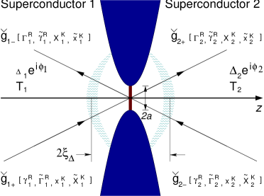
Figure 1: Geometry of the temperature-biased Josephson contact of radius $a$. There is a potential barrier at $z=0$ with transparency $D({\bf p}_{f})$, which connects trajectories with positive and negative projection of the Fermi momentum on the ${\bf z}$-axis. The labels indicate which Ricatti amplitudes are computed along each trajectory. The shaded boundaries define the region ($\sim\xi_{\text{\tiny$\Delta$}}\gg a$) where superconductivity and the excitation spectrum are strongly modified for $\phi_{1}\neq\phi_{2}$.

We consider two superconductors, denoted 1 and 2, or $L$ (left) and $R$ (right), connected through a small constriction of diameter $2a$ at $z=0$, see Fig. 1. The constriction is assumed to be much smaller than the superconductor coherence length,

$$2a\ll\xi_{\text{\tiny$\Delta$}}=\frac{v_{f}}{\pi\Delta}\,,$$ (1)

as well as the elastic mean free path, $\ell$, and inelastic mean free path, $\ell_{\text{\tiny in}}$. We will consider the ballistic limit, $\ell\gg\xi_{\text{\tiny$\Delta$}}$ in Section III and the diffusive limit $\ell\ll\xi_{\text{\tiny$\Delta$}}$ in Section VI. In all cases, we assume that the inelastic mean free path is much larger than any other length scale in the problem.

The potential barrier at $z=0$ (the vertical line in Fig. 1) is characterized by a transmission probability, $D({\bf p}_{f})$ for normal-state quasiparticles with Fermi momentum ${\bf p}_{f}$ incident on the interface. The reflection probabilty is given by $R({\bf p}_{f})=1-D({\bf p}_{f})$. The angle-dependence of $D({\bf p}_{f})$ depends on the microscopic barrier and is not very important for our purposes; we use a $\delta$-function barrier which gives,

$$D({\bf p}_{f})=\frac{D_{0}\cos^{2}\theta}{1-D_{0}\sin^{2}\theta},$$ (2)

where $\theta=\arccos(\hat{{\bf v}}_{f}\cdot\hat{z})$ is the angle between quasiparticle trajectory and interface normal, ${\bf v}_{f}$ is the Fermi velocity and $D_{0}$ is the transmission probability for quasiparticles incident normal to the interface. We develop the theory for heat conduction for arbitrary transparency of the constriction: $0<D_{0}\leq 1$. This theory describes a variety of Josephson weak links, including the tunnel junction ($D_{0}\ll 1$) and the pin-hole point contact ($D_{0}=1$).

For the order parameters of the two superconductors, we restrict ourselves to the singlet pairing case, but keep the orbital symmetry arbitrary. Thus, the order parameter is in general assumed to be of the form $i\sigma_{y}\Delta({\bf p}_{f})$, where $\sigma_{y}$ is the second Pauli matrix in spin space and $\Delta({\bf p}_{f})$ is the momentum dependent gap amplitude. The results reported below for the heat transport are for low-$T_{c}$ superconductors with isotropic order parameters. However, the formalism is applicable to a broader range of Josephson contacts, including anisotropic or unconventional spin-singlet pairing states. We note that current conservation is only guaranteed if the propagators and self-energies (order parameter, impurity self-energy, etc.) are calculated self-consistently. In the point-contact geometry we can neglect the back-action of the current on the self-energies to lowest order in the small parameter $a/\xi_{\Delta}$.Kulik and Omeĺyanchuk (1978)

The electrical and thermal resistances of the junction, both $\propto a^{-2}$, are much larger than the corresponding resistances of the leads. Thus, the phase change, as well as the temperature change, occur essentially at the junction. We then take the local phases and temperatures near the contact to be equal to the reservoir phases and temperatures. Thus, we write the order parameters as $\Delta_{1}(T_{1})\,e^{i\phi_{1}}$ and $\Delta_{2}(T_{2})\,e^{i\phi_{2}}$ in superconductor $1$ and $2$, respectively. Here are the local temperatures near the contact given by $T_{1}$ and $T_{2}$, respectively. We define the phase difference over the junction $\phi=\phi_{2}-\phi_{1}$ and the temperature bias ${\mbox{\footnotesize$\Delta$}}T=T_{2}-T_{1}$. In the linear response we will write $T_{1}=T$ and $T_{2}=T+{\mbox{\footnotesize$\Delta$}}T$.

III Ballistic case

To study the transport of quasiparticles through superconducting point contacts as described above, we use the method of nonequilibrium quasiclassical Green functions.Eliashberg (1972); Larkin and Ovchinnikov (1975, 1977); Serene and Rainer (1983); Rammer and Smith (1986) In this formalism the advanced and retarded Green functions, $\hat{\mathfrak{G}}^{A,R}$, describe the local spectrum of excitations of the system, while the Keldysh Green functions, $\hat{\mathfrak{G}}^{K}$, carry information about the nonequilibrium population of these states. The propagators $\hat{\mathfrak{G}}^{A,R,K}({\bf p}_{f},{\bf R};\epsilon,t)$ are $4\times 4$ matrices in Nambu (particle-hole and spin) space and obey transport-like equations for excitations of energy $\epsilon$ moving along classical trajectories labelled by the Fermi momentum ${\bf p}_{f}$. The temperature- and phase-biased contact is, to quasiclassical accuracy, in a stationary state; thus, we drop the dependence on $t$.

The heat current through the point contact ${\bf I}_{\epsilon}(\phi,T_{1},T_{2})$ is a function of the phase difference $\phi$ and the bath temperatures $T_{1}$ and $T_{2}$. In our geometry, the heat current flows along the junction normal only, ${\bf I}_{\epsilon}=\hat{z}\text{I}_{\epsilon}$, and is found by energy integration and Fermi-surface averaging of the quasiclassical Keldysh Green’s function. Current conservation allows us to write the heat current in terms of functions locally at the junction on trajectories with positive and negative projections of the Fermi momentum on the $\hat{\bf z}$-axis: $\hat{\mathfrak{G}}^{K}_{+}=\hat{\mathfrak{G}}^{K}({\bf p}_{f}\cdot\hat{z}>0,\epsilon;\phi,T_{1},T_{2})$ and $\hat{\mathfrak{G}}^{K}_{-}=\hat{\mathfrak{G}}^{K}({\bf p}_{f}\cdot\hat{z}<0,\epsilon;\phi,T_{1},T_{2})$, respectively. Thus,

$$\begin{split}\text{I}_{\epsilon}(\phi,T_{1},T_{2})&={\cal A}N_{f}v_{f}\;\int_{-\infty}^{\infty}\frac{d\epsilon}{4\pi i}\;\epsilon\\ &\times\left\langle\text{Tr}\left[\hat{\mathfrak{G}}^{K}_{+}-\hat{\mathfrak{G}}^{K}_{-}\right]\right\rangle,\end{split}$$ (3)

where $N_{f}$ is the normal-state density of states at the Fermi level, ${\cal A}=\pi a^{2}$ is the cross-sectional area of the contact, and the angle brackets denote a Fermi-surface average, including the projection of the group velocity along the direction normal to the interface.

A efficient method of computing the Green’s functions is provided by the parametrization in terms of generalized spectral functions $i\sigma_{y}\gamma^{R}$ and distribution functions $x^{K}$, which are $2\times 2$ matrices in spin space. In the spin-singlet case, the spin structure of the spectral functions are all given by $i\sigma_{y}$, while the distribution functions are proportional to the unit matrix. These scalar amplitudes obey Ricatti-type differential equations.Nagato et al. (1993); Schopohl and Maki (1995); Eschrig et al. (1999) Each Green’s function can be written in terms of a set of Ricatti amplitudes. The retarded and advanced Green functions have the forms

$$\begin{split}&\hat{\mathfrak{G}}^{R,A}[\gamma^{R,A},\tilde{\gamma}^{R,A}]=\\ &\frac{\mp\pi i}{\zeta^{R,A}}\left(\begin{array}[]{cc}1-\gamma^{R,A}\tilde{\gamma}^{R,A}&2i\sigma_{y}\gamma^{R,A}\\ -2i\sigma_{y}\tilde{\gamma}^{R,A}&-1+\tilde{\gamma}^{R,A}\gamma^{R,A}\end{array}\right),\end{split}$$ (4)

where $\zeta^{R,A}=1+\gamma^{R,A}\tilde{\gamma}^{R,A}$, while the the Keldysh Green function has the form

$$\hat{\mathfrak{G}}^{K}[\gamma^{R},\tilde{\gamma}^{R},\gamma^{A},\tilde{\gamma}^{A},x^{K},\tilde{x}^{K}]=\qquad\qquad\qquad\qquad$$ (5)

$$\frac{-2\pi i}{\zeta^{R}\zeta^{A}}\left(\begin{array}[]{cc}x^{K}+\tilde{x}^{K}\gamma^{R}\tilde{\gamma}^{A}&i\sigma_{y}(x^{K}\gamma^{A}-\tilde{x}^{K}\gamma^{R})\\ -i\sigma_{y}(x^{K}\tilde{\gamma}^{R}-\tilde{x}^{K}\tilde{\gamma}^{A})&\tilde{x}^{K}+x^{K}\tilde{\gamma}^{R}\gamma^{A}\end{array}\right)\,.$$ (8)

The advanced amplitudes are related to the retarded ones through the symmetry $\gamma^{A}=-(\tilde{\gamma}^{R})^{*}$. We will also make use of the conjugation symmetrySerene and Rainer (1983)

$$\tilde{q}({\bf p}_{f},z,\epsilon)=q(-{\bf p}_{f},z,-\epsilon)^{*}\,.$$ (9)

For each trajectory, the spectral functions and distribution functions are found by integrating the corresponding Ricatti equations with initial condition either in the bulk or at the interface, depending on the stability properties of the differential equation. We follow the notation in Ref. Eschrig, 2000; quantities denoted by lower case letters are computed by integrating the Ricatti equations with initial conditions in the bulk, while quantities denoted with upper case letters are computed by integrating the Ricatti equations with initial conditions at the interface. According to this convention, for each of the four trajectories in Fig. 1, we change lower case letters in Eqs. 4-5 to upper case letters; the list of amplitudes defining each Keldysh Green function for the scattering trajectories are shown in Fig. 1.

In the bulk region, the amplitudes are given by their equilibrium values

$$\begin{split}\gamma^{R}_{j}({\bf p}_{f},\epsilon)&=-\frac{\Delta_{j}({\bf p}_{f})e^{i\phi_{j}}}{\varepsilon^{R}+i\sqrt{\Delta_{j}({\bf p}_{f})^{2}-(\varepsilon^{R})^{2}}},\\ \tilde{\gamma}^{R}_{j}({\bf p}_{f},\epsilon)&=\frac{\Delta_{j}({\bf p}_{f})e^{-i\phi_{j}}}{\varepsilon^{R}+i\sqrt{\Delta_{j}({\bf p}_{f})^{2}-(\varepsilon^{R})^{2}}},\\ x^{K}_{j}({\bf p}_{f},\epsilon)&=(1-|\gamma^{R}_{j}({\bf p}_{f},\epsilon)|^{2})\tanh{\frac{\epsilon}{2T_{j}}},\\ \tilde{x}^{K}_{j}({\bf p}_{f},\epsilon)&=-(1-|\tilde{\gamma}^{R}_{j}({\bf p}_{f},\epsilon)|^{2})\tanh{\frac{\epsilon}{2T_{j}}},\end{split}$$ (10)

where the index $j=1,\;2$ refers to quantities in superconductor one (two). Both $\varepsilon^{R}$ and the mean field gap $\Delta_{j}$ formally include renormalization effects (self-energies) from elastic and inelastic scattering. In the following we consider the ballistic (clean) case and defer the discussion of impurity scattering to Sec. VI. We also assume that the inelastic scattering rate, $\Gamma_{\text{\tiny in}}$, is small compared to all relevant energy scales. We can then write $\varepsilon^{R}=\epsilon+i\Gamma_{\text{\tiny in}}\rightarrow\epsilon+i0^{+}$, and $\Delta_{j}$ denotes the temperature-dependent weak-coupling gap amplitude.

The lower case amplitudes are found by integrating the Ricatti equations from the bulk to the interface, with the initial conditions in Eqs. 10. The initial conditions for the upper case Ricatti amplitudes at the contact are then found from Zaitsev’s non-linear boundary conditions,Zaĭtsev (1984) which in terms of Ricatti amplitudes are reduced to linear boundary conditions.Eschrig (2000) For the distribution functions we use the notation in Ref. Löfwander et al., 2003 and obtain,

$$\begin{split}X_{1}^{K}&=R_{ee}x_{1}^{K}+\bar{T}_{ee}x_{2}^{K}+(-\bar{T}_{eh})\tilde{x}_{2}^{K},\\ \tilde{X}_{1}^{K}&=R_{hh}\tilde{x}_{1}^{K}+(-\bar{T}_{he})x_{2}^{K}+\bar{T}_{hh}\tilde{x}_{2}^{K},\\ X_{2}^{K}&=T_{ee}x_{1}^{K}+(-T_{eh})\tilde{x}_{1}^{K}+\bar{R}_{ee}x_{2}^{K},\\ \tilde{X}_{2}^{K}&=(-T_{he})x_{1}^{K}+T_{hh}\tilde{x}_{1}^{K}+\bar{R}_{hh}\tilde{x}_{2}^{K}.\end{split}$$ (11)

In terms of the following particle-hole spinor notation,

$$|\alpha\rangle=\left(\begin{array}[]{c}1\\ -i\sigma_{y}\alpha\end{array}\right),\hskip 28.45274pt\langle\alpha|=\left(1,\;\;-i\sigma_{y}\alpha^{*}\right),$$ (12)

the Green’s functions at the junction ($z=0$) can be written in a compact form

$$\begin{split}\hat{\mathfrak{G}}^{K}_{1+}&=-\frac{2\pi i}{N_{1}}\left[x_{1}^{K}|r_{he}\rangle\langle r_{he}|+\tilde{X}_{1}^{K}\hat{\tau}_{1}|\gamma^{R}_{1}\rangle\langle\gamma^{R}_{1}|\hat{\tau}_{1}\right],\\ \hat{\mathfrak{G}}^{K}_{1-}&=-\frac{2\pi i}{N_{2}}\left[\tilde{x}_{1}^{K}\hat{\tau}_{1}|r_{eh}\rangle\langle r_{eh}|\hat{\tau}_{1}+X_{1}^{K}|\tilde{\gamma}^{R}_{1}\rangle\langle\tilde{\gamma}^{R}_{1}|\right],\\ \hat{\mathfrak{G}}^{K}_{2-}&=-\frac{2\pi i}{N_{3}}\left[x_{2}^{K}|\bar{r}_{he}\rangle\langle\bar{r}_{he}|+\tilde{X}_{2}^{K}\hat{\tau}_{1}|\gamma^{R}_{2}\rangle\langle\gamma^{R}_{2}|\hat{\tau}_{1}\right],\\ \hat{\mathfrak{G}}^{K}_{2+}&=-\frac{2\pi i}{N_{4}}\left[\tilde{x}_{2}^{K}\hat{\tau}_{1}|\bar{r}_{eh}\rangle\langle\bar{r}_{eh}|\hat{\tau}_{1}+X_{2}^{K}|\tilde{\gamma}^{R}_{2}\rangle\langle\tilde{\gamma}^{R}_{2}|\right],\end{split}$$ (13)

where $N_{k}=|\zeta_{k}|^{2}$ for $k=1...4$ with

$$\zeta_{1} =1+\gamma^{R}_{1}r_{he}\,, \zeta_{3} =1+\gamma^{R}_{2}\bar{r}_{he}\,,$$ (14)

$$\zeta_{2} =1+\tilde{\gamma}^{R}_{1}r_{eh}\,, \zeta_{4} =1+\tilde{\gamma}^{R}_{2}\bar{r}_{eh}\,.$$

The Andreev reflection amplitudes $r_{\alpha\beta}$ are listed in Table 1, and the scattering probabilities, $T_{\alpha\beta}$ and $R_{\alpha\beta}$, are listed in Table 2. The notation is chosen such that $T^{R}_{\alpha\beta}$ ($R^{R}_{\alpha\beta}$) denotes the probability of transmission (reflection) of a particle of type $\beta$ to a particle of type $\alpha$. Quantities with a bar denote transmission from right to left and reflection on the right side, while those without bar denote transmission from left to right and reflection on the left side.

Table 1: The Andreev reflection probabilities. The denominators are listed in Table 2.

$r_{he}=\tilde{\Gamma}^{R}_{1}=[R(1+\tilde{\gamma}^{R}_{2}\gamma^{R}_{2})\tilde{\gamma}^{R}_{1}+D(1+\tilde{\gamma}^{R}_{1}\gamma^{R}_{2})\tilde{\gamma}^{R}_{2}]/B_{1}$

$r_{eh}=\Gamma^{R}_{1}=[R(1+\gamma^{R}_{2}\tilde{\gamma}^{R}_{2})\gamma^{R}_{1}+D(1+\gamma^{R}_{1}\tilde{\gamma}^{R}_{2})\gamma^{R}_{2}]/B_{2}$

$\bar{r}_{he}=\tilde{\Gamma}^{R}_{2}=[R(1+\gamma^{R}_{1}\tilde{\gamma}^{R}_{1})\tilde{\gamma}^{R}_{2}+D(1+\tilde{\gamma}^{R}_{2}\gamma^{R}_{1})\tilde{\gamma}^{R}_{1}]/B_{3}$

$\bar{r}_{eh}=\Gamma^{R}_{2}=[R(1+\gamma^{R}_{1}\tilde{\gamma}^{R}_{1})\gamma^{R}_{2}+D(1+\gamma^{R}_{2}\tilde{\gamma}^{R}_{1})\gamma^{R}_{1}]/B_{4}$

Table 2: Scattering probabilities for $x^{K}$ distribution functions in the stationary SIS junction setup.

$\bar{T}_{hh}=D|1+\tilde{\gamma}^{R}_{1}\gamma^{R}_{2}|^{2}/|B_{1}|^{2}$	$\bar{T}_{he}=RD|\tilde{\gamma}^{R}_{1}-\tilde{\gamma}^{R}_{2}|^{2}/|B_{1}|^{2}$	$R_{hh}=R|1+\tilde{\gamma}^{R}_{2}\gamma^{R}_{2}|^{2}/|B_{1}|^{2}$	$B_{1}=1+R\gamma^{R}_{2}\tilde{\gamma}^{R}_{2}+D\tilde{\gamma}^{R}_{1}\gamma^{R}_{2}$
$\bar{T}_{ee}=D|1+\gamma^{R}_{1}\tilde{\gamma}^{R}_{2}|^{2}/|B_{2}|^{2}$	$\bar{T}_{eh}=RD|\gamma^{R}_{1}-\gamma^{R}_{2}|^{2}/|B_{2}|^{2}$	$R_{ee}=R|1+\gamma^{R}_{2}\tilde{\gamma}^{R}_{2}|^{2}/|B_{2}|^{2}$	$B_{2}=1+R\gamma^{R}_{2}\tilde{\gamma}^{R}_{2}+D\gamma^{R}_{1}\tilde{\gamma}^{R}_{2}$
$T_{hh}=D|1+\tilde{\gamma}^{R}_{2}\gamma^{R}_{1}|^{2}/|B_{3}|^{2}$	$T_{he}=RD|\tilde{\gamma}^{R}_{2}-\tilde{\gamma}^{R}_{1}|^{2}/|B_{3}|^{2}$	$\bar{R}_{hh}=R|1+\gamma^{R}_{1}\tilde{\gamma}^{R}_{1}|^{2}/|B_{3}|^{2}$	$B_{3}=1+R\gamma^{R}_{1}\tilde{\gamma}^{R}_{1}+D\tilde{\gamma}^{R}_{2}\gamma^{R}_{1}$
$T_{ee}=D|1+\gamma^{R}_{2}\tilde{\gamma}^{R}_{1}|^{2}/|B_{4}|^{2}$	$T_{eh}=RD|\gamma^{R}_{2}-\gamma^{R}_{1}|^{2}/|B_{4}|^{2}$	$\bar{R}_{ee}=R|1+\gamma^{R}_{1}\tilde{\gamma}^{R}_{1}|^{2}/|B_{4}|^{2}$	$B_{4}=1+R\gamma^{R}_{1}\tilde{\gamma}^{R}_{1}+D\gamma^{R}_{2}\tilde{\gamma}^{R}_{1}$

We use the above interface Green functions to compute the heat current via Eq. 3. There are four contributions, one for each incoming distribution function in Eq. 10: $i=1-4$ for $x^{K}_{1},\tilde{x}^{K}_{1},x^{K}_{2},\tilde{x}^{K}_{2}$, corresponding to electron-like and hole-like quasiparticles injected from the left ($i=1-2$) and right ($i=3-4$) reservoirs,

$$\text{I}_{\epsilon}=\int_{-\infty}^{\infty}d\epsilon\left\langle\sum_{i=1}^{4}j_{\epsilon}^{i}({\bf p}_{f},z,\epsilon;\phi)\right\rangle\,.$$ (15)

We can express the spectral current in terms of transmission probabilities, $T^{R}_{\alpha\beta}$, for the distribution functions. The most direct way of achieving this is to make use of the unitarity of the scattering matrix for the junction, which leads to the relation

$$\begin{split}&\text{Tr}\left[\hat{\mathfrak{G}}^{K}_{+}({\bf p}_{f},z=0^{-},\epsilon)-\hat{\mathfrak{G}}^{K}_{-}({\bf p}_{f},z=0^{-},\epsilon)\right]\\ &=\text{Tr}\left[\hat{\mathfrak{G}}^{K}_{+}({\bf p}_{f},z=0^{+},\epsilon)-\hat{\mathfrak{G}}^{K}_{-}({\bf p}_{f},z=0^{+},\epsilon)\right].\end{split}$$ (16)

Thus, we compute $j_{\epsilon}^{1}$ and $j_{\epsilon}^{2}$ at $z=0^{+}$, while $j_{\epsilon}^{3}$ and $j_{\epsilon}^{4}$ are computed at $z=0^{-}$. The heat current spectral densities can then be written as

$$\begin{split}j_{\epsilon}^{1}({\bf p}_{f},z=0^{+},\epsilon;\phi,T_{1},T_{2})&=-{\cal A}N_{f}v_{f}\epsilon\,x^{K}_{1}\left[T_{ee}(1-|\tilde{\gamma}^{R}_{2}|^{2})N_{4}^{-1}+T_{he}(1-|\gamma^{R}_{2}|^{2})N_{3}^{-1}\right],\\ j_{\epsilon}^{2}({\bf p}_{f},z=0^{+},\epsilon;\phi,T_{1},T_{2})&=-{\cal A}N_{f}v_{f}\epsilon\,\tilde{x}^{K}_{1}\left[-T_{eh}(1-|\tilde{\gamma}^{R}_{2}|^{2})N_{4}^{-1}-T_{hh}(1-|\gamma^{R}_{2}|^{2})N_{3}^{-1}\right],\\ j_{\epsilon}^{3}({\bf p}_{f},z=0^{-},\epsilon;\phi,T_{1},T_{2})&=-{\cal A}N_{f}v_{f}\epsilon\,x^{K}_{2}\left[-\bar{T}_{he}(1-|\gamma^{R}_{1}|^{2})N_{1}^{-1}-\bar{T}_{ee}(1-|\tilde{\gamma}^{R}_{1}|^{2})N_{2}^{-1}\right],\\ j_{\epsilon}^{4}({\bf p}_{f},z=0^{-},\epsilon;\phi,T_{1},T_{2})&=-{\cal A}N_{f}v_{f}\epsilon\,\tilde{x}^{K}_{2}\left[\bar{T}_{hh}(1-|\gamma^{R}_{1}|^{2})N_{1}^{-1}+\bar{T}_{eh}(1-|\tilde{\gamma}^{R}_{1}|^{2})N_{2}^{-1}\right].\end{split}$$ (17)

Note that each spectral current density vanishes in the subgap region, i.e. for $|\epsilon|<\max(\Delta_{1},\Delta_{2})$ the factor $1-|\gamma^{R}|^{2}=0$. The heat current is only carried by continuum energy quasiparticles, and thus, we only consider $|\epsilon|>\max(\Delta_{1},\Delta_{2})$ from here on. Using the symmetry in Eq. 9 we obtain

$$\begin{split}j_{\epsilon}^{2}({\bf p}_{f},z=0^{+},\epsilon)&=j_{\epsilon}^{1}(-{\bf p}_{f},z=0^{+},-\epsilon),\\ j_{\epsilon}^{4}({\bf p}_{f},z=0^{-},\epsilon)&=j_{\epsilon}^{3}(-{\bf p}_{f},z=0^{-},-\epsilon),\end{split}$$ (18)

which implies that hole-like quasiparticles carry the same amount of heat as the electron-like quasiparticles (after energy integration and Fermi-surface averaging).

We introduce transmission coefficients (script $\mathfrak{D}$’s) by combining the scattering probabilities for $x^{K}$ distribution functions (big $T$’s) with the spectral renormalization factors [the factors, $(1-|\gamma^{R}|^{2})$, and the denominators $N^{-1}_{i}$]. We then obtain,

$$\begin{split}j_{\epsilon}^{1}&=-{\cal A}N_{f}v_{f}\epsilon\,\tanh\frac{\epsilon}{2T_{1}}\left[\mathfrak{D}_{ee}({\bf p}_{f},\epsilon)+\mathfrak{D}_{he}({\bf p}_{f},\epsilon)\right],\\ j_{\epsilon}^{3}&=+{\cal A}N_{f}v_{f}\epsilon\,\tanh\frac{\epsilon}{2T_{2}}\left[\bar{\mathfrak{D}}_{ee}({\bf p}_{f},\epsilon)+\bar{\mathfrak{D}}_{he}({\bf p}_{f},\epsilon)\right].\end{split}$$ (19)

The transmission coefficient for electron-like quasiparticles remaining electron-like, $\mathfrak{D}_{ee}$, has the form

$$\begin{split}\mathfrak{D}_{ee}({\bf p}_{f},\epsilon)&=(1-|\gamma^{R}_{1}|^{2})T_{ee}(1-|\tilde{\gamma}^{R}_{2}|^{2})N_{4}^{-1}\\ &=\frac{D(1-|\gamma^{R}_{1}|^{2})(1-|\tilde{\gamma}^{R}_{2}|^{2})|1+\gamma^{R}_{2}\tilde{\gamma}^{R}_{1}|^{2}}{|Z|^{2}},\end{split}$$ (20)

while the transmission coefficient for electron-like quasiparticles with branch conversion to hole-like quasiparticles, $\mathfrak{D}_{he}$, is

$$\mathfrak{D}_{he}({\bf p}_{f},\epsilon)=\frac{RD(1-|\gamma^{R}_{1}|^{2})(1-|\gamma^{R}_{2}|^{2})|\tilde{\gamma}^{R}_{2}-\tilde{\gamma}^{R}_{1}|^{2}}{|Z|^{2}}.$$ (21)

The corresponding coefficients for transmission from right to left are,

$$\begin{split}\bar{\mathfrak{D}}_{ee}({\bf p}_{f},\epsilon)&=\frac{D(1-|\gamma^{R}_{2}|^{2})(1-|\tilde{\gamma}^{R}_{1}|^{2})|1+\gamma^{R}_{1}\tilde{\gamma}^{R}_{2}|^{2}}{|Z|^{2}},\\ \bar{\mathfrak{D}}_{he}({\bf p}_{f},\epsilon)&=\frac{RD(1-|\gamma^{R}_{2}|^{2})(1-|\gamma^{R}_{1}|^{2})|\tilde{\gamma}^{R}_{1}-\tilde{\gamma}^{R}_{2}|^{2}}{|Z|^{2}}.\end{split}$$ (22)

The common denominator is given by

$$\begin{split}Z=&1+R(\gamma^{R}_{1}\tilde{\gamma}^{R}_{1}+\gamma^{R}_{2}\tilde{\gamma}^{R}_{2})\\ &+D(\gamma^{R}_{1}\tilde{\gamma}^{R}_{2}+\tilde{\gamma}^{R}_{1}\gamma^{R}_{2})+\gamma^{R}_{1}\tilde{\gamma}^{R}_{1}\gamma^{R}_{2}\tilde{\gamma}^{R}_{2}.\end{split}$$ (23)

We immediately see that

$$\bar{\mathfrak{D}}_{he}({\bf p}_{f},\epsilon)=\mathfrak{D}_{he}({\bf p}_{f},\epsilon),$$ (24)

while the symmetry given by Eq. 9 leads to

$$\bar{\mathfrak{D}}_{ee}({\bf p}_{f},\epsilon)=\mathfrak{D}_{ee}(-{\bf p}_{f},-\epsilon).$$ (25)

With the aid of these relations we can express the total heat current in a more compact form,

$$\text{I}_{\epsilon}(\phi,T_{1},T_{2})=2\int_{\max(\Delta)}^{\infty}d\epsilon\;j_{\epsilon}(z=0,\epsilon;\phi,T_{1},T_{2}),$$ (26)

where the factor $2$ reflects the symmetry of the spectral current under $-\epsilon\to\epsilon$. The heat-current spectral density is expressed in terms of the Fermi-surface averaged transmission coefficient,

$$\begin{split}j_{\epsilon}(z=0,\epsilon;\phi,T_{1},T_{2})&=-2{\cal A}N_{f}v_{f}\epsilon\;\Big{\langle}\mathfrak{D}({\bf p}_{f},\epsilon,\phi;T_{1},T_{2})\Big{\rangle}\\ &\quad\left[\tanh\frac{\epsilon}{2T_{1}}-\tanh\frac{\epsilon}{2T_{2}}\right]\,,\end{split}$$ (27)

$$\mathfrak{D}({\bf p}_{f},\epsilon,\phi)=\mathfrak{D}_{ee}({\bf p}_{f},\epsilon,\phi)+\mathfrak{D}_{he}({\bf p}_{f},\epsilon,\phi)\,,$$ (28)

where the factor two is due to the electron-hole symmetry [c.f. Eq. 18]. Equation 26 satisfies the symmetries

$$\begin{split}\text{I}_{\epsilon}(-\phi,T_{1},T_{2})&=\text{I}_{\epsilon}(\phi,T_{1},T_{2}),\\ \text{I}_{\epsilon}(\phi,T_{2},T_{1})&=-\text{I}_{\epsilon}(\phi,T_{1},T_{2}).\end{split}$$ (29)

and Eqs. 26-27 are the results for non-linear heat-current response to a temperature and phase bias. These results hold for singlet superconductors with any orbital symmetry, in particular for either $s$-wave or $d$-wave symmetries.

III.1 S-wave symmetry: $\Delta({\bf p}_{f})=\Delta$

In the remaining sections we focus on the low-$T_{c}$ superconductors, with a momentum independent ($s$-wave) order parameter. However, the order parameters for the two superconductors have different phases, $\phi_{j}$, and may also have different order parameter amplitudes, e.g. as a result of a finite temperature bias, $\Delta_{j}=\Delta(T_{j})$. The retarded Ricatti amplitudes in the bulk are then momentum independent. Moreover, since the s-wave order parameter is constant in space for the point contact, the lower case Ricatti amplitudes are given by their bulk values along the whole trajectory. We then obtain analytic expressions for the effective transmission coefficients

$$\begin{split}\mathfrak{D}_{ee}({\bf p}_{f},\epsilon)&=\frac{2D\xi_{1}\xi_{2}(\epsilon^{2}+\xi_{1}\xi_{2}-\Delta_{1}\Delta_{2}\cos\phi)}{\left[D\epsilon^{2}+(1+R)\xi_{1}\xi_{2}-D\Delta_{1}\Delta_{2}\cos\phi\right]^{2}},\\ \mathfrak{D}_{he}({\bf p}_{f},\epsilon)&=\frac{2RD\xi_{1}\xi_{2}(\epsilon^{2}-\xi_{1}\xi_{2}-\Delta_{1}\Delta_{2}\cos\phi}{\left[D\epsilon^{2}+(1+R)\xi_{1}\xi_{2}-D\Delta_{1}\Delta_{2}\cos\phi\right]^{2}}.\end{split}$$ (30)

where $\xi_{j}\equiv\text{sgn}(\epsilon)\sqrt{\epsilon^{2}-\Delta_{j}^{2}}$.

III.2 Linear response

In linear response we write $T_{1}=T$ and $T_{2}=T+\delta T$. Then to lowest order in $\delta T$ we obtain,

$$I_{\epsilon}(\phi,T)=-\kappa(\phi,T)\,\delta T,$$ (31)

where the heat conductance has the form

$$\kappa(\phi,T)=4{\cal A}\int_{\Delta}^{\infty}d\epsilon{\cal N}(\epsilon)[\epsilon v_{g}(\epsilon)]\left\langle\mathfrak{D}(\epsilon,\phi,T)\right\rangle\,\left(\frac{\partial f}{\partial T}\right),$$ (32)

with the transmission coefficient,

$$\mathfrak{D}({\bf p}_{f},\epsilon,\phi,T)=\mathfrak{D}_{ee}({\bf p}_{f},\epsilon,\phi,T)+\mathfrak{D}_{he}({\bf p}_{f},\epsilon,\phi,T)\,,$$ (33)

$$\begin{split}\mathfrak{D}_{ee}({\bf p}_{f},\epsilon,\phi,T)&=D\frac{(\epsilon^{2}-\Delta^{2})(\epsilon^{2}-\Delta^{2}\cos^{2}\frac{\phi}{2})}{\left[\epsilon^{2}-\Delta^{2}(1-D\sin^{2}\frac{\phi}{2})\right]^{2}},\\ \mathfrak{D}_{he}({\bf p}_{f},\epsilon,\phi,T)&=RD\frac{(\epsilon^{2}-\Delta^{2})\,\Delta^{2}\sin^{2}\frac{\phi}{2}}{\left[\epsilon^{2}-\Delta^{2}(1-D\sin^{2}\frac{\phi}{2})\right]^{2}}.\end{split}$$ (34)

Equation 32 is an intuitive form of the heat conductance that resembles the bulk thermal conductivity. The conductance is expressed in terms of the bulk quasiparticle density of states, ${\cal N}(\epsilon)=N_{f}|\epsilon|/\sqrt{\epsilon^{2}-\Delta^{2}}$, and the energy current carried by these quasiparticles, $[\epsilon\,v_{g}(\epsilon)]$, where $v_{g}(\epsilon)=v_{f}\sqrt{\epsilon^{2}-\Delta^{2}}/|\epsilon|$ is the group velocity of a bulk excitation. Note that the product, ${\cal N}v_{g}=N_{f}v_{f}$, is energy independent. The backscattering at the junction (resulting from the Sharvin resistance and the transparency $D\leq 1$), which limits the heat conductance, corresponds to the elastic mean free path due to impurities in the bulk.

The linear response results in Eqs. 31-33 for the heat conductance were reported in Ref. Zhao et al., 2003, for a ${\bf p}_{f}$-independent normal-state transmission probability, $D$. In Sec. IV we extend the analysis of the linear response limit and examine the non-linear thermal response, Eqs. 26-27, in Sec. V.

IV Thermal Conductance

The phase modulation of the heat conductance, $\kappa(\phi,T)$, is determined by the transmission coefficient, $\mathfrak{D}(\epsilon,\phi,T)$. The energy dependence of the transmission coefficient reflects features of the phase-dependent local density of states (LDOS) of the junction, ${\cal N}_{J}(\epsilon,\phi,T)$. The LDOS at the contact is defined as ${\cal N}_{J}({\bf p}_{f},\epsilon,\phi,T)=-\frac{N_{f}}{\pi}\text{Im}\hat{\mathfrak{G}}^{R}_{11}({\bf p}_{f},z=0^{-},\epsilon,\phi,T)$, where $\hat{\mathfrak{G}}^{R}_{11}$ is the diagonal (11) component of the retarded Green’s function, which has the following form at the junction,

$$\frac{\hat{\mathfrak{G}}^{R}_{11}({\bf p}_{f},z=0^{-},\epsilon)}{-i\pi}=\frac{\epsilon\sqrt{\Delta^{2}-\epsilon^{2}}-\frac{i}{2}\text{sgn}({\bf p}_{f}\cdot\hat{\bf z})\Delta^{2}D\sin\phi}{\epsilon^{2}-\Delta^{2}(1-D\sin^{2}\frac{\phi}{2})}\,.$$ (35)

The resulting LDOS has both a bound-state ($|\epsilon|<\Delta$) and continuum ($|\epsilon|>\Delta$) spectrum given by

$$\frac{{\cal N}_{J}({\bf p}_{f},\epsilon,\phi,T)}{{\cal N}_{f}} =\Theta(|\epsilon|-\Delta)\frac{|\epsilon|\sqrt{\epsilon^{2}-\Delta^{2}}}{\epsilon^{2}-\Delta^{2}(1-D\sin^{2}(\phi/2))}$$ (36)

$$\quad+\pi\delta(\epsilon-\epsilon_{B})\frac{|\epsilon|\sqrt{\Delta^{2}-\epsilon^{2}}-\frac{1}{2}\text{sgn}({\bf p}_{f}\cdot\hat{\bf z})\Delta^{2}D\sin\phi}{2|\epsilon|}+\pi\delta(\epsilon+\epsilon_{B})\frac{|\epsilon|\sqrt{\Delta^{2}-\epsilon^{2}}+\frac{1}{2}\text{sgn}({\bf p}_{f}\cdot\hat{\bf z})\Delta^{2}D\sin\phi}{2|\epsilon|},$$

The spectrum is shown in Fig. 2 as a function of the phase bias (2c) and as a function of barrier transparency for $\phi=\pi$ (2a). Of particular importance is the formation of a pair of Andreev bound states (ABS) with phase dispersion

$$\epsilon_{B}=\pm\Delta\sqrt{1-D\sin^{2}\frac{\phi}{2}}\,,$$ (37)

and the impact of the ABS on the continuum spectrum.

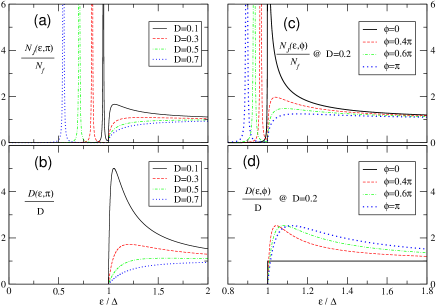
Figure 2: The LDOS at the junction, $N_{J}(\epsilon,\phi)$, and the transmission coefficient, $\mathfrak{D}(\epsilon,\phi)$, at fixed momentum ${\bf p}_{f}$ with $D\equiv D({\bf p}_{f})$. (a)-(b) Different transparencies at phase difference $\phi=\pi$. (c)-(d) Different phase differences at transparency $D=0.2$. $N_{J}$ is suppressed by the formation of the ABS, as $\phi$ is tuned from $0$ to $\pi$. For high transparency $\mathfrak{D}$ is suppressed, but for low transparency $\mathfrak{D}$ contains a resonance at $\epsilon_{r}\simeq\Delta+\frac{1}{2}\Delta D\sin^{2}\frac{\phi}{2}$, at which $\mathfrak{D}(\epsilon_{r},\phi)=1/2$. In all cases, $T=0.72T_{c}$, and for clarity we added a small width, $\sim 10^{-3}T_{c}$ to the bound-states.

In addition, we note the following characteristics of the LDOS:

1. In the absence of phase bias, $\phi=0$, the LDOS reduces to the BCS density of states in the bulk.

2. Under a phase bias, $\phi\neq 0$, Andreev bound states are formed, with spectral weight drawn from the continuum near $\epsilon=\Delta$.

3. The ABS are weakly bound and close to the continuum edge for low transparency. For high transparency these states are more strongly bound, and may lie well below the gap.

4. For $\phi=\pi$ the ABS is the closest to the Fermi level (at $\epsilon_{B}=\Delta\sqrt{R}$), and consequently the spectral weight of continuum excitations is reduced the most at this phase bias.

These characteristics of the LDOS have direct consequences for the properties of the transmission coefficient, $\mathfrak{D}$, and thus for the heat conductance. For $\phi=0$ the transmission coefficient becomes independent of energy and reduces to the normal-state transmission probability: $\mathfrak{D}(\epsilon,0)=D$. Thus, the thermal conductance of the point contact at $\phi=0$,

$$\kappa(\phi=0)=\frac{N_{f}v_{f}\,\langle D\rangle\,{\cal A}}{T^{2}}\int_{\Delta}^{\infty}d\epsilon\epsilon^{2}\mathrm{sech}^{2}\frac{\epsilon}{2T}\,,$$ (38)

is reduced compared to the normal-state conductance (Eq. 38 with $\Delta=0$), $\kappa_{\text{N}}=\frac{2\pi^{2}}{3}N_{f}v_{f}\,\langle D\rangle\,{\cal A}\,T$, by opening the superconducting gap. Note that the temperature dependence of the ratio, $\kappa(\phi=0)/\kappa_{\text{N}}(T_{c})$, is equivalent to that of the normalized bulk thermal conductivity of an s-wave BCS superconductor.

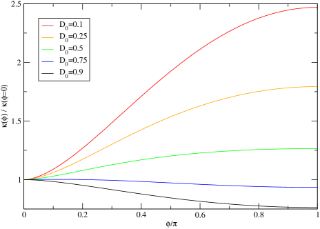
Figure 3: The thermal conductance as a function of $\phi$ and barrier transparency $D$. The thermal conductance is normalized for each $D$ by its value at $\phi=0$.

For $\phi\neq 0$, the transmission coefficient is strongly dependent on energy and phase, which is the source of the phase-modulation of the thermal conductance shown in Fig. 3. For high transparency ($D\gtrsim 0.7$), the suppression of the continuum density of states associated with the formation of the ABS well below the gap is reflected in a suppressed transmission coefficient and a reduced heat conductance compared to $\phi=0$. Thus, for high transparency as $\phi$ is tuned from $0$ to $\pi$, the conductance is suppressed as shown in Fig. 3. In the limit $D\rightarrow 1$ only direct transmission is possible, $\mathfrak{D}_{ee}(\epsilon,\phi)=(\epsilon^{2}-\Delta^{2})/(\epsilon^{2}-\Delta^{2}\cos^{2}(\frac{\phi}{2}))$; branch conversion processes vanish, $\mathfrak{D}_{he}=0$, and we recover the heat conductance of a pinhole junction

$$\kappa(\phi)=\frac{N_{f}v_{f}{\cal A}}{4T^{2}}\int_{\Delta}^{\infty}d\epsilon\frac{\epsilon^{2}(\epsilon^{2}-\Delta^{2})}{\epsilon^{2}-\Delta^{2}\cos^{2}\frac{\phi}{2}}\mathrm{sech}^{2}\frac{\epsilon}{2T}\,,$$ (39)

obtained by Kulik and Omelyanchuk.Kulik and Omeĺyanchuk (1992)

In the case of low transparency, $D\ll 1$, and $\phi\neq 0$, the Andreev bound states lie just below the gap edge. The transmission coefficient, $\mathfrak{D}(\epsilon,\phi)$, exhibits a resonance just above the gap edge, as shown in Fig. 2. This resonance is a consequence of the shallow ABS. We see this fact clearly in Fig. 2(c)-(d): the continuum LDOS is reduced as $\phi$ is changed from $0$ to $\pi$, while the resonance in the transmission coefficient is enhanced (the area under the curve is enhanced). The resonance energy is obtained by writing $\epsilon_{r}=\Delta+\delta\epsilon_{r}$, where $\delta\epsilon_{r}\ll\Delta$, in the expression for the transmission coefficient, Eq. 33. From the extremum condition, $\partial\mathfrak{D}/\partial\,\delta\epsilon_{r}=0$, we obtain

$$\epsilon_{r}\approx\Delta\left(1+\frac{1}{2}D\sin^{2}\frac{\phi}{2}\right).$$ (40)

At the resonance energy the transmission coefficient is independent of transparency and takes the value

$$\mathfrak{D}(\epsilon_{r},\phi)=\frac{1}{2}.$$ (41)

The resonant transmission of quasiparticles with energies $\epsilon\approx\epsilon_{\text{r}}$ leads to an increase in the thermal conductance as the phase bias is tuned from $0$ to $\pi$, as shown in Fig. 3. Observation of the phase modulation may be accomplished with a point-contact Josephson junction in a SQUID geometry. In this case the phase is tuned by the flux, $\Phi$, threading the SQUID, $\phi=2\pi(\Phi/\Phi_{0})$, where $\Phi_{0}=hc/2e$ is the superconducting flux quantum.

Another important consequence of the resonance is the increase of the thermal conductance for $\phi=\pi$ compared to the normal-state conductance at $T_{c}$, as the temperature is lowered below $T_{c}$, see Fig. 4. This peak effect is large and persists over a broad temperature range, $0.5T_{c}\lesssim T\leq T_{c}$, for moderate to low transparencies, $D\sim 0.2$ to $D\ll 1$.

For very low temperatures, $T\ll\Delta$, the sharpening of the distribution functions at the Fermi level, combined with the gap in the continuum spectrum leads to an exponentially small thermal conductance. The reduction of the low-temperature heat conductance for normal-superconducting (NS) proximity structures is well known from Andreev’s work on heat reflection at NS interfaces.Andreev (1964) However, the increase in the thermal conductance compared to the normal state in the intermediate to high temperature range is not related to Andreev reflection at high-transparency interfaces, but is a consequence resonant transmission of heat carrying quasiparticles, and is characteristic of intermediate- to low-transparency Josephson point-contact junctions.

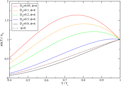
Figure 4: The temperature dependence of phase-modulation of the thermal conductance for $\phi=\pi$, normalized by the conductance at $T_{c}$, $\kappa_{N}=2\pi^{2}{\cal A}N_{f}v_{f}T_{c}\left<D\right>/3$. Shown for comparison is the normalized conductance for $\phi=0$, which is independent of transparency.

IV.1 The tunnelling limit: $D\to 0$

Here we examine in more detail the phase dependence of the thermal conductance in Eq. 32 in the tunnelling limit, $D\ll 1$. We neglect the momentum dependence and set $D({\bf p}_{f})=D$. For $D\ll 1$, when we expand the transmission coefficient, $\mathfrak{D}(\epsilon,\phi)$, to leading order in $D$ there is prefactor proportional to $D$, and a non-perturbative dependence on $D$ that is responsible for the resonance peak at $\epsilon_{\text{r}}$. The resonance leads to a non-analytic contribution to the conductance proportional $D\ln D$ that dominates in the limit $D\to 0$. Consequently up to order $D$ the thermal conductance $\kappa(\phi)$ contains a term proportional to $\sin^{2}{\phi\over 2}$, as well as a nonanalytic term proportional to $\sin^{2}{\phi\over 2}\ln(\sin^{2}{\phi\over 2})$,

$$\kappa(\phi)=\kappa_{0}-\kappa_{1}\sin^{2}\frac{\phi}{2}\ln(\sin^{2}\frac{\phi}{2})+\kappa_{2}\sin^{2}\frac{\phi}{2}\,,$$ (42)

where $\kappa_{0}$ is given by Eq. 38 and

$$\kappa_{1}={N_{f}v_{f}D{\cal A}\Delta^{3}\over 4T^{2}}\mathrm{sech}^{2}{\Delta\over 2T},$$

$$\kappa_{2}={N_{f}v_{f}D{\cal A}\Delta^{3}\over 4T^{2}}\left[{4T\over\Delta}(1-\tanh{\Delta\over 2T})+c\right]-(1+\ln D)\kappa_{1},$$

$$c=2\int_{0}^{\infty}dxx\ln x\left[{{\Delta\over T}\;\mathrm{sinh}{\sqrt{x^{2}+1}\over 2T/\Delta}\over(x^{2}+1)\mathrm{cosh}^{3}{\sqrt{x^{2}+1}\over 2T/\Delta}}+{\mathrm{sech}^{2}{\sqrt{x^{2}+1}\over 2T/\Delta}\over(x^{2}+1)^{3/2}}\right].$$

The phase modulation of the thermal conductance is shown in the inset of Fig. 5, the term $\kappa_{2}\sin^{2}{\phi\over 2}$ and the term $-\kappa_{1}\sin^{2}{\phi\over 2}\ln(\sin^{2}{\phi\over 2})$ are plotted separately for $T=0.5T_{c}$ and $D=0.01$. The relative importance of the two terms is shown for $D=0.01$ and $D=0.005$ as a function of temperature. The ratio $\kappa_{1}/\kappa_{2}$ increases as temperature is lowered.

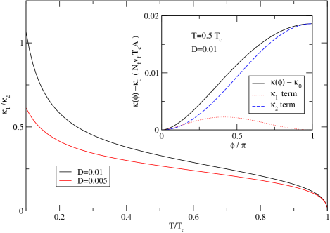
Figure 5: The ratio $\kappa_{1}/\kappa_{2}$ as a function of temperature. The inset shows the phase dependence of the thermal conductance, the contributions from terms proportional to $\kappa_{1}$ and $\kappa_{2}$ are plotted separately.

We compare Eq. 42 with the result obtained with the tunnelling Hamiltonian (tH) method (see Refs. Guttman et al., 1997, 1998 and Appendix). According to the tH calculation, the heat transport through a tunnel junctions is given by Eq. 55 in the Appendix. In the linear response limit, $\delta T\rightarrow 0$, $\Delta_{1}=\Delta_{2}$, and Eq. 55 reduces to

$$\kappa^{\mathrm{tH}}(\phi)=8\pi N_{f}^{2}|{\bf T}|^{2}\int^{+\infty}_{\Delta}d\epsilon\;\epsilon{\partial f(\epsilon)\over\partial T}{\epsilon^{2}-\Delta^{2}\cos\phi\over\epsilon^{2}-\Delta^{2}}.$$ (43)

The integral in Eq. 43 is divergent due to the singularity at $\epsilon=\Delta$. The divergence is unphysical and indicative of the failure of low-order perturbation theory within the tH method for the linear response. What is missing in Eq. 43 is the correction to the spectrum - which enters the denominator - that results from the small, but finite, barrier transparency. This non-perturbative correction is fully taken into account in the quasiclassical Green function method. The singularity of the DOS at $\epsilon=\Delta$ is removed by the formation of the ABS, and the final result, Eqs. 32-33, contain no divergence in the linear response limit.

In earlier treatments the divergence entering the tH result was regulated by introducing an ad-hoc cutoff,Guttman et al. (1997, 1998) for example by requiring that the two gaps have different magnitudes, $\Delta_{1}\neq\Delta_{2}$. Under these circumstances, Eq. 55 predicts the thermal conductance has the form $\kappa(\phi)=\kappa^{\prime}_{0}-\kappa^{\prime}_{2}\cos\phi$, with both $\kappa^{\prime}_{0}$ and $\kappa^{\prime}_{2}$ proportional to $|{\bf T}|^{2}\propto D$. However, as shown in Eq. 42 the thermal conductance of a tunnel junction contains non-perturbative corrections to the cosine dependence, i.e. the leading order correction is $-\kappa_{1}\sin^{2}{\phi\over 2}\ln(\sin^{2}{\phi\over 2})$. Also the magnitude of $\kappa_{2}$ contains a term proportional to $D\ln D$.

V Non-linear response

When we consider the non-linear response one important effect is that the order parameters on the two sides have different magnitudes,

$$\begin{split}\Delta_{1}&=\Delta(T),\\ \Delta_{2}&=\Delta(T+{\mbox{\footnotesize$\Delta$}}T)<\Delta_{1}.\end{split}$$ (44)

The density of states is modified accordingly. There are three important regions of the local excitation spectrum (c.f. Fig. 6):

1. $|\epsilon|<\Delta_{2}$, sub-gap spectrum with bound states,

2. $\Delta_{2}<|\epsilon|<\Delta_{1}$, semi-continuum spectrum,

3. $\Delta_{1}<|\epsilon|$, true continuum spectrum.

Only the states in the true continuum carry heat. In Fig. 7 we plot the local density of states at the junction for three different phase differences. The difference between the gap magnitudes becomes large as ${\mbox{\footnotesize$\Delta$}}T$ is increased, the bound states move closer to the semi-continuum edge. At the same time, the true continuum edge is further separated from the ABS. Consequently, the true continuum is less affected by the bound states, and therefore the phase bias.

Figure 6: Three regions in energy: sub-gap energies below the gap of both superconducting leads, semi-continuum energies between the two gap energies, and the true continuum. Only the true continuum states transport heat.

The Andreev bound states also have an impact on the heat current in the non-linear response, via a mirror effect in the continuum which introduces a resonance in the transmission coefficient. However, in the non-linear response, the true continuum is shielded from the bound state by the semi-continuum. This weakens the resonance and suppresses the signatures of resonant transmission in the heat current. The transmission coefficient is plotted in Fig. 8(c). For low transparency, the resonance is weakened when ${\mbox{\footnotesize$\Delta$}}T$ is increased. More specifically, the area under the transmission curve, which is the relevant quantity for the heat current, is reduced. For high transparency, the opposite happens: the transmission coefficients is less suppressed near the gap edge as ${\mbox{\footnotesize$\Delta$}}T$ is increased (not shown).

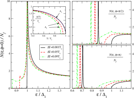
Figure 7: Local density of states at the junction at $z=0^{-}$ in the non-linear response, for transparency $D=0.5$ and temperature $T=0.72T_{c}$.

In addition to the spectral change found in $\mathfrak{D}$, the change of the thermal occupation factors for the two reservoirs influences the heat transfer. We have checked that the main effect on the heat current is due to the spectral change, but the change in the occupation factors reduces the overall effect of a phase bias on the heat current. The total heat transfer is larger for a larger temperature bias, but we eliminate this scale factor by normalizing the heat current by the corresponding heat current at zero phase bias, or at $T_{c}$.

The phase-modulation of the heat current is plotted in Fig. 8(b), while the temperature dependence is shown in Fig. 8(a). Since the angle dependence of the barrier transparency does not qualitatively affect our results, we use the angle-independent model. The phase-modulation is weakened, and the peak effect near $T_{c}$ for low transparency and phase difference $\phi=\pi$ is reduced. However, the non-linearity does not remove or drastically alter the resonance effects, and the main features found in linear response persist for finite temperature bias.

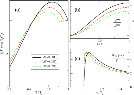
Figure 8: (a) Temperature dependence and (b) phase dependence of the heat current in the non-linear response. (c) Transmission coefficient in the non-linear response at phase bias $\phi=\pi$. In (b)-(c) the temperature is $T=0.72T_{c}$, and in all cases the transparency of the junction is $D=0.1$.

VI Diffusive case

In this section we discuss the case where the two leads are dirty superconductors, i.e. the elastic mean free path, $\ell\ll\xi_{\text{\tiny$\Delta$}}$. In dirty superconductors, $\check{\mathfrak{G}}(\mathbf{p}_{f})$ is nearly isotropic, and

$$\check{g}({\bf R};\epsilon)={1\over-i\pi}\int{d\Omega_{{\bf p}_{f}}\over 4\pi}\check{\mathfrak{G}}({\bf p}_{f},{\bf R};\epsilon,)=\left(\begin{array}[]{cc}\hat{g}^{R}&\hat{g}^{K}\\ 0&\hat{g}^{A}\end{array}\right)\,,$$ (45)

satisfies the Usadel diffusion-type equation.Usadel (1970) The isotropic propagator determines most of the physical observables. For example, the heat current density is given by

$$\mathbf{j}_{\epsilon}={N_{f}v_{f}\ell\over 12}\int d\epsilon\,\epsilon\,\mathrm{Tr}(\check{g}\text{\boldmath$\nabla$}\check{g})^{K}.$$ (46)

To calculate the heat current through the point contact with dirty leads, we need the boundary conditions for the isotropic propagator, $\check{g}$, at an interface. Such boundary conditions were derived by Nazarov in the formulation of the circuit theory of diffusive hetero-structures.Nazarov (1999) In this model the contact is described by a set of transmission eigenvalues, $\{D_{n}\}$, or equivalently a distribution function, $\rho(D)$. The boundary conditions are

$$N_{f1}v_{f1}\ell_{1}\check{g}_{1}\partial_{z}\check{g}_{1}=N_{f2}v_{f2}\ell_{2}\check{g}_{2}\partial_{z}\check{g}_{2}\,,$$ (47)

$${2\pi\over 3}{\cal A}N_{f2}v_{f2}\ell_{2}\check{g}_{2}\partial_{z}\check{g}_{2}=\int dD\rho(D)\check{I}\,,$$ (48)

where the Keldysh matrix $\check{I}$ is defined as

$$\check{I}\equiv{2D[\check{g}_{2},\check{g}_{1}]\over 4+D(\{\check{g}_{2},\check{g}_{1}\}-2)}\,,$$ (49)

$N_{fi}$ is the normal-state density of states at the Fermi level of lead $i=1$, $2$, $v_{fi}$ is the Fermi velocity of lead $i$, and ${\cal A}$ is the cross-sectional area of the contact interface. Eq. 47 is the conservation of spectral current, and Eqs. 46-48 imply that the total heat current through the contact can be calculated from $\check{I}$,

$$\text{I}_{\epsilon}={1\over 8\pi}\int d\epsilon\epsilon\int dD\rho(D)\,\mathrm{Tr}(\hat{I}^{K})\,.$$ (50)

The Keldysh component of $\check{I}$ can be worked out to beNazarov (1999)

$$\hat{I}^{K} = {D\hat{g}^{R}_{1}\hat{g}^{K}_{2}\over 2-D+D\{\hat{g}^{R}_{1},\hat{g}^{R}_{2}\}/2}+{D\hat{g}^{K}_{1}\hat{g}^{A}_{2}\over 2-D+D\{\hat{g}^{A}_{1},\hat{g}^{A}_{2}\}/2}$$

$$- {D^{2}(\hat{g}^{R}_{1}\hat{g}^{K}_{2}\hat{g}^{A}_{1}\hat{g}^{A}_{2}+\hat{g}^{R}_{1}\hat{g}^{R}_{2}\hat{g}^{K}_{1}\hat{g}^{A}_{2}+2\hat{g}^{K}_{2}\hat{g}^{A}_{2})\over 2(2-D+D\{\hat{g}^{R}_{1},\hat{g}^{R}_{2}\}/2)(2-D+D\{\hat{g}^{A}_{1},\hat{g}^{A}_{2}\}/2)}$$

$$- (1\leftrightarrow 2),$$

where $(1\leftrightarrow 2)$ means the exchange of index 1 and 2 in all three terms.

For point contacts, we approximate $\hat{g}_{i}^{R,A,K}$ with their bulk values, e.g. $\hat{g}^{K}_{i}=(\hat{g}^{R}_{i}-\hat{g}^{A}_{i})\tanh({\epsilon/2T_{i}})$. We focus on the linear response, assume that superconducting leads 1 and 2 have the same gap and evaluate the conductance in the limit $\delta T\rightarrow 0$. After some algebra we find

$$I_{\epsilon}=-{\delta T\over 2\pi T^{2}}\int_{\Delta}^{\infty}d\epsilon\int dD\rho(D)\epsilon^{2}(\epsilon^{2}-\Delta^{2})\mathrm{sech}^{2}{\epsilon\over 2T}$$

$$\times{D(\epsilon^{2}-\Delta^{2}\cos{\phi\over 2})+DR\Delta^{2}\sin^{2}(\phi/2)\over[\epsilon^{2}-\Delta^{2}+D\Delta^{2}\sin^{2}(\phi/2)]^{2}}\,.$$ (51)

Notice that with the replacement,

$$\int dD\rho(D)(...)\Rightarrow 2\pi{\cal A}N_{f}v_{f}\langle...\rangle\,,$$ (52)

the result for the conductance with diffusive leads, Eq. 51, in the limit of a narrow distribution of transmission barriers, is the exactly the same as Eqs. 31-33 for the conductance obtained in the ballistic limit.

The near equivalence of the conductances for the diffusive and ballistic limits is related in part to the small expansion parameter, $a/\xi_{\text{\tiny$\Delta$}}$. In this limit pairbreaking effects resulting from the current flow in the vicinity of the junction can be neglected, and as a result the impurity renormalization of the excitation energy and order parameter cancel for s-wave superconductors. The resulting thermal conductance of point contact is then insensitive to impurity scattering in the leads. This result is not expected to hold for larger area contacts with $a\gtrsim\xi_{\text{\tiny$\Delta$}}$. These junctions are beyond the scope of this work.

VII Conclusions

We have derived a general expression for the phase- and temperature-dependent thermal current through small Josephson weak links. The results are valid for arbitrary transparency of the junction. In the ballistic limit, we obtained an expression for the heat current in terms of a transmission coefficient, $\mathfrak{D}(\epsilon,\phi,T_{1},T_{2})$, for heat transport by continuum quasiparticle states. The transmission coefficient includes direct transmission processes, $\mathfrak{D}_{ee}$, and transmission processes with branch conversion, $\mathfrak{D}_{he}$. The phase modulation, temperature dependence, and the dependence on the barrier transparency of the heat current can be understood intuitively in terms of the properties of the transmission coefficient.

In linear response, for high transparencies, the suppression of the continuum density of states associated with the formation of a low-energy Andreev bound state leads to a suppression of the transmission coefficient, and the thermal conductance, as the phase difference across the junction is tuned from $0$ to $\pi$. As a consequence, the thermal conductance drops below the conductance for $\phi=0$ for temperatures below $T_{c}$.

However, for intermediate to low transparencies, a resonance develops in the transmission coefficient as the phase difference is tuned from $0$ to $\pi$. Consequently, the conductance is larger at $\phi=\pi$ than at $\phi=0$. The transmission resonance is due to the ABS being close to the gap edge. This effect is similar to transmission resonances found in wave mechanics for a quantum well with a shallow bound state just below the continuum edge. For $\phi=\pi$ the resonance in the heat current leads to an increase in the thermal conductance compared to the normal-state conductance at $T_{c}$, over a broad temperature region below $T_{c}$.

In the low-transparency limit, $D\ll 1$, we derived an analytic expression for the heat conductance and found that there are non-analytic corrections, of type $D\ln D$, to the usual linear in $D$ term. Also the phase dependence contains non-analytic terms of the form $\sin^{2}\frac{\phi}{2}\ln(\sin^{2}\frac{\phi}{2})$. The first-order tunnel Hamiltonian method gives a divergent result in linear response, which is regulated by the formation of an Andreev bound state from the continuum states near $\epsilon=\Delta$. A similar divergence occurs in the sub-harmonic gap structure (SGS) of the current-voltage characteristics of a superconducting tunnel junction when the sub-gap structure is computed to finite order in perturbation theory within the tunnel Hamiltonian method.Schrieffer and Wilkins (1963) In the case of the SGS, summation to infinite order within a wave-function method,Bratus et al. (1995); Averin and Bardas (1995) or the tH method,Cuevas et al. (1996) regulates the divergences. Such a summation is possible for the thermal conductance within the tH method. However, the quasiclassical Green’s function method with the interface boundary conditions includes the bound-state spectrum so unphysical divergences never appear.

We also studied the case when the superconducting leads are in the diffusive limit. Based on the junction boundary conditions developed by Nazarov, we found that the heat conductance has the same form as in the ballistic case.

Finally, in the non-linear response we find that the resonance in the transmission coefficient is reduced by the presence of the semi-continuum spectrum, which shields the extended continuum energy quasiparticle states carrying heat from the ABS. The effects found in the linear response are reduced, but not dramatically. Thus, we conclude that it is not essential to be in the linear response limit in order to observe the resonance effects in the heat current.

*

Appendix A Perturbation Theory

We review the first-order perturbation calculation of the heat current for low-transparency junctions based on the tunnelling Hamiltonian (tH) method.Ambegaokar and Baratoff (1963) Consider two superconductors, labelled by $L$ and $R$, weakly coupled by an insulating layer. They are assumed to be described by the Hamiltonian

$$H_{total}=H_{0}+H_{T},$$

where $H_{0}$ is the sum of the BCS reduced Hamiltonian of superconductors $L$ and $R$,

$$H_{0}=H_{L}+H_{R},$$

$$H_{L}=\sum_{p,\sigma}\epsilon_{p}c^{\dagger}_{p,\sigma}c_{p,\sigma}+{1\over 2}\sum_{p,p^{\prime},\sigma}V_{pp^{\prime}}c^{\dagger}_{p,\sigma}c^{\dagger}_{-p,-\sigma}c_{-p^{\prime},-\sigma}c_{p^{\prime},\sigma},$$

$$H_{R}=\sum_{k,\sigma}\epsilon_{k}a^{\dagger}_{k,\sigma}a_{k,\sigma}+{1\over 2}\sum_{k,k^{\prime},\sigma}V_{kk^{\prime}}a^{\dagger}_{k,\sigma}a^{\dagger}_{-k,-\sigma}a_{-k^{\prime},-\sigma}c_{k^{\prime},\sigma},$$

and $H_{T}$ describes the tunnelling processes,

$$H_{T}=\sum_{k,p,\sigma}[T_{kp}a{\dagger}_{k,\sigma}c_{p\sigma}+h.c.].$$

The two superconductors are also assumed to be at the same chemical potential $\mu_{L}=\mu_{R}$, but at different temperatures $T_{L}\neq T_{R}$.

The momentum index, $p$, and the annihilation operator, $c_{p,\sigma}$, are reserved for superconductor $L$, while index, $k$, and operator, $a_{k,\sigma}$, are reserved for superconductor $R$. The spin state is labelled by $\sigma$, and $T_{kp}$ is the tunnelling matrix element. With the BCS approximation, $V_{pp^{\prime}}=\lambda<0$, the order parameter is defined as

$$\Delta_{L}=-\lambda\sum_{p}\left<c_{-p,-\sigma}c_{p,\sigma}\right>=|\Delta_{L}|e^{i\phi_{L}}.$$

The heat current operator is defined as

$$I_{\epsilon}=-{\partial Q_{L}\over\partial t}=-i[H_{total},Q_{L}]=-i[H_{T},Q_{L}],$$

$$Q_{L}=H_{L}-\mu_{L}\sum_{p,\sigma}c^{\dagger}_{p,\sigma}c_{p,\sigma}.$$

It is straightforward to work out the commutator $[H_{T},Q_{L}]$. Within the mean field approximation, the pair annihilation operator $c_{-q,-\sigma}c_{q,\sigma}$ reduces to its average value, and we find

$$I_{\epsilon}=-i\sum_{k,p,\sigma}\left[T_{kp}\xi_{p}a^{\dagger}_{k,\sigma}c_{p,\sigma}-T_{kp}\Delta_{L}a^{\dagger}_{k,\sigma}c^{\dagger}_{-p,-\sigma}-h.c.\right],$$ (53)

with $\xi_{p}=\epsilon_{p}-\mu_{L}$.

To calculate the ensemble average of the operator $I_{\epsilon}$, we use the interaction picture and treat $H_{T}$ as a perturbation to $H_{0}$. According to first order perturbation theory, the heat current has the form

$$\text{I}_{\epsilon}=\langle I_{\epsilon}\rangle=-i\int_{-\infty}^{t}dt^{\prime}e^{\eta t^{\prime}}\left<\left[\mathcal{I}_{\epsilon}(t),\mathcal{H}_{T}(t^{\prime})\right]\right>_{0},$$

where $\mathcal{I}_{\epsilon}(t)$ and $\mathcal{H}_{T}(t^{\prime})$ are the operators in the interaction picture corresponding to $I_{\epsilon}$ and $H_{T}$. respectively. The ensemble average $\left<...\right>_{0}$ is defined by $H_{0}$, and $\eta=0^{+}$. The commutator $[\mathcal{I}_{\epsilon}(t),\mathcal{H}_{T}(t^{\prime})]$ contains various correlation functions,

$$\text{I}_{\epsilon}=-\int_{-\infty}^{\infty}dt^{\prime}e^{\eta t^{\prime}}\Theta(t-t^{\prime})\sum_{i,j=1,2}[C_{ij}(t,t^{\prime})+h.c.],$$

where we define $C_{ij}(t,t^{\prime})=\left<[\mathcal{O}_{i}(t),\mathcal{P}_{j}(t^{\prime})]\right>_{0}$ with

$$\mathcal{O}_{1}(t)=\sum_{k,p,\sigma}T_{kp}\xi_{p}a^{\dagger}_{k,\sigma}(t)c_{p,\sigma}(t),$$

$$\mathcal{O}_{2}(t)=-\sum_{k,p,\sigma}T_{kp}\Delta_{L}a^{\dagger}_{k,\sigma}(t)c^{\dagger}_{-p,-\sigma}(t),$$

$$\mathcal{P}_{1}(t)=\sum_{k,p,\sigma}T_{kp}a^{\dagger}_{k,\sigma}(t)c_{p,\sigma}(t),$$

$$\mathcal{P}_{2}(t)=\mathcal{P}_{1}^{\dagger}(t),$$

and $a_{k,\sigma}(t)$ and $c_{p,\sigma}(t)$ are annihilation operators in the interaction picture. We introduce the following single-particle correlation functions,

$$G^{>}_{p,\sigma}(t,t^{\prime})=-i\left<c_{p,\sigma}(t)c^{\dagger}_{p,\sigma}(t^{\prime})\right>_{0},$$

$$G^{<}_{p,\sigma}(t,t^{\prime})=+i\left<c^{\dagger}_{p,\sigma}(t^{\prime})c_{p,\sigma}(t)\right>_{0},$$

$$F^{>}_{p,\sigma}(t,t^{\prime})=-i\left<c_{-p,-\sigma}(t)c_{p,\sigma}(t^{\prime})\right>_{0},$$

$$F^{<}_{p,\sigma}(t,t^{\prime})=+i\left<c_{p,\sigma}(t^{\prime})c_{-p,-\sigma}(t)\right>_{0},$$

$$\bar{F}^{>}_{p,\sigma}(t,t^{\prime})=-i\left<c^{\dagger}_{p,\sigma}(t)c^{\dagger}_{-p,-\sigma}(t^{\prime})\right>_{0},$$

$$\bar{F}^{<}_{p,\sigma}(t,t^{\prime})=+i\left<c^{\dagger}_{-p,-\sigma}(t^{\prime})c^{\dagger}_{p,\sigma}(t)\right>_{0}.$$

The correlation functions, $C_{ij}$, can then be decomposed into $G$’s and $F$’s with the aid of Wick’s theorem. For example,

$$C_{11}(t,t^{\prime})=-\sum_{k,p,\sigma}T_{kp}T_{-k-p}\xi_{p}$$

$$\times[\bar{F}^{>}_{k,\sigma}(t,t^{\prime})F^{<}_{p,\sigma}(t^{\prime},t)-\bar{F}^{<}_{k,\sigma}(t,t^{\prime})F^{>}_{p,\sigma}(t^{\prime},t)].$$

The contribution of $C_{11}$ to the heat current is

$$\text{I}_{11} = -\int_{-\infty}^{\infty}dt^{\prime}e^{\eta t^{\prime}}\Theta(t-t^{\prime})C_{11}(t,t^{\prime})$$

$$= -2i\sum_{k,p}T_{kp}T_{-k-p}\xi_{p}\int{d\omega\over 2\pi}\int{d\omega^{\prime}\over 2\pi}$$

$$[f_{L}(\omega)-f_{R}(\omega^{\prime})]{B(p,\omega)\bar{B}(k,\omega^{\prime})\over\omega^{\prime}-\omega-i\eta}.$$

The factor 2 comes from the sum over spin, and $A$ and $B$ are spectral functions, with

$$G^{\gtrless}_{p}(\omega)=\mp if_{L}(\mp\omega)A(p,\omega),$$

$$F^{\gtrless}_{p}(\omega)=\mp if_{L}(\mp\omega)B(p,\omega),$$

$$\bar{F}^{\gtrless}_{p}(\omega)=\mp if_{L}(\mp\omega)\bar{B}(p,\omega).$$

Here we introduced the Fermi function $f_{L}(\omega)=(e^{\omega/T_{L}}+1)^{-1}$, and the spectral functions

$$A(p,\omega)=\pi[(1+{\xi_{p}\over E_{p}})\delta(\omega-E_{p})+(1-{\xi_{p}\over E_{p}})\delta(\omega+E_{p})],$$

$$B(p,\omega)=\pi{\Delta_{L}\over E_{p}}[\delta(\omega-E_{p})-\delta(\omega+E_{p})],$$

$$\bar{B}(p,\omega)=B^{*}(p,\omega),$$

with $E_{p}=(\xi_{p}^{2}+\Delta_{L}^{2})^{1/2}$. Analogous calculations for the other correlation functions follow. Summing up all the contributions for the heat current gives

$$\text{I}_{\epsilon}=-4\,\mathrm{Im}\sum_{k,p}\int{d\omega\over 2\pi}\int{d\omega^{\prime}\over 2\pi}[f_{L}(\omega)-f_{R}(\omega^{\prime})]\times$$

$$\Big{\{}|T_{kp}|^{2}\xi_{p}{A(p,\omega)A(k,\omega^{\prime})\over\omega^{\prime}-\omega+i\eta}+|T_{kp}|^{2}\Delta_{L}{\bar{B}(-p,\omega)A(k,\omega^{\prime})\over\omega^{\prime}-\omega+i\eta}$$

$$-T_{kp}T_{-k-p}\xi_{p}{B(p,\omega)\bar{B}(k,\omega^{\prime})\over\omega^{\prime}-\omega-i\eta}$$

$$+T_{kp}T_{-k-p}\Delta_{L}{A(-p,\omega)\bar{B}(k,\omega^{\prime})\over\omega^{\prime}-\omega-i\eta}\Big{\}}.$$ (54)

In Eq. 54 we neglect the momentum dependence of the tunnelling matrix elements, put $T_{kp}\rightarrow{\bf T}$, and change the momentum sum into integrals over excitation energies $E_{p}$ and $E_{k}$. The integrals over $\omega$ and $\omega^{\prime}$ collapse because of the $\delta$ functions in the spectral functions $A$, $B$ and $\bar{B}$. Taking the imaginary part of the integrand yields new $\delta$ functions $\delta(E_{k}\pm E_{p})$, which lead to a collapse of one of the energy integrals. Finally, the heat current takes the form

$$I_{\epsilon}=8\pi N_{f}^{L}N_{f}^{R}|{\bf T}|^{2}\int^{+\infty}_{\Delta_{\mathrm{max}}}d\epsilon\;\epsilon[f_{L}(\epsilon)-f_{R}(\epsilon)]$$

$$\times{\epsilon^{2}-|\Delta_{L}||\Delta_{R}|\cos\phi\over\sqrt{\epsilon^{2}-|\Delta_{L}|^{2}}\sqrt{\epsilon^{2}-|\Delta_{R}|^{2}}}.$$ (55)

Here the phase difference, $\phi=\phi_{L}-\phi_{R}$, $\Delta_{\mathrm{max}}=\mathrm{max}[|\Delta_{L}|,|\Delta_{R}|]$, and $N_{f}^{L/R}$ are the density of states at the Fermi level for $L$ and $R$ sides, respectively.

Finally, we compare with previous calculations of the heat current in tunnel junctions. In Ref. Maki and Griffin, 1965 only the kinetic energy term was included in deriving the current operator; the term, $T_{kp}\Delta_{L}a^{\dagger}_{k,\sigma}c^{\dagger}_{-p,-\sigma}$, and its Hermitian conjugate were missing from Eq. 53. In the main result of Guttman et al. (Eq. 9 of Ref. Guttman et al. (1997)) the sign of the $\cos\phi$ term is incorrect.

———————————————————————– ———————————————————————–

References

• Belzig et al. (1999) W. Belzig, F. K. Wilhelm, C. Bruder, G. Schön, and A. Zaikin, Superlatt. Microstruct. 25, 1251 (1999).
• Agrait et al. (2003) N. Agrait, A. L. Yeyati, and J. M. van Ruitenbeek, Phys. Rep. 377, 81 (2003).
• Aumentado et al. (1999) J. Aumentado, V. Chandrasekhar, J. Eom, P. M. Baldo, and L. E. Rehn, Appl. Phys. Lett. 75, 3554 (1999).
• Zhao et al. (2003) E. Zhao, T. Löfwander, and J. A. Sauls, arXiv/cond-mat/ 0302346, 4 (2003), [to appear in PRL, 2003].
• Eschrig et al. (1999) M. Eschrig, J. A. Sauls, and D. Rainer, Phys. Rev. B 60, 10447 (1999).
• Eschrig (2000) M. Eschrig, Phys. Rev. B 61, 9061 (2000).
• Josephson (1962) B. D. Josephson, Phys. Lett. 1, 251 (1962).
• Arnold (1987) G. B. Arnold, J. Low Temp. Phys. 68, 1 (1987).
• Andreev (1965) A. F. Andreev, Zh. Eksp. Teor. Fiz. 49, 655 (1965), [Sov Phys JETP 22 455].
• Andreev (1964) A. F. Andreev, Zh. Eksp. Teor. Fiz. 46, 1823 (1964), [Sov Phys JETP 19 1228 (1964)].
• Maki and Griffin (1965) K. Maki and A. Griffin, Phys. Rev. Lett. 15, 921 (1965).
• Guttman et al. (1997) G. D. Guttman, B. Nathanson, E. Ben-Jacob, and D. J. Bergman, Phys. Rev. B 55, 3849 (1997).
• Guttman et al. (1998) G. D. Guttman, E. Ben-Jacob, and D. J. Bergman, Phys. Rev. B 57, 2717 (1998).
• Kulik and Omeĺyanchuk (1978) I. Kulik and A. Omeĺyanchuk, Sov. J. Low Temp. Phys. 4, 142 (1978).
• Eliashberg (1972) G. M. Eliashberg, Zh. Eskp. Teor. Fiz. 61, 1254 (1972), [English translation Sov. Phys. JETP 34, 668 (1972)].
• Larkin and Ovchinnikov (1975) A. Larkin and Y. Ovchinnikov, Zh. Eskp. Teor. Fiz. 68, 1915 (1975), [English translation Sov. Phys. JETP 41, 960 (1976)].
• Larkin and Ovchinnikov (1977) A. Larkin and Y. Ovchinnikov, Zh. Eskp. Teor. Fiz. 73, 299 (1977), [English translation Sov. Phys. JETP 46, 155 (1978)].
• Rammer and Smith (1986) J. Rammer and H. Smith, Rev. Mod. Phys. 58, 323 (1986).
• Serene and Rainer (1983) J. W. Serene and D. Rainer, Phys. Rep. 101, 221 (1983).
• Nagato et al. (1993) Y. Nagato, K. Nagai, and J. Hara, J. Low Temp. Phys. 93, 33 (1993).
• Schopohl and Maki (1995) N. Schopohl and K. Maki, Physica B 204, 214 (1995).
• Zaĭtsev (1984) A. V. Zaĭtsev, Sov. Phys. JETP 59, 1015 (1984).
• Löfwander et al. (2003) T. Löfwander, M. Fogelström, and J. A. Sauls, arXiv/cond-mat/ 0304588, 15 (2003), [to appear in PRB, 2003].
• Kulik and Omeĺyanchuk (1992) I. Kulik and A. Omeĺyanchuk, Sov. J. Low Temp. Phys. 18, 819 (1992).
• Usadel (1970) K. Usadel, Phys. Rev. Lett. 25, 507 (1970).
• Nazarov (1999) Y. V. Nazarov, Superlatt. Microstruc. 25, 1221 (1999), [also in cond-mat/9811155].
• Schrieffer and Wilkins (1963) J. R. Schrieffer and J. W. Wilkins, Phys. Rev. Lett. 10, 17 (1963).
• Bratus et al. (1995) E. N. Bratus, V. S. Shumeiko, and G. Wendin, Phys. Rev. Lett. 74, 2110 (1995).
• Averin and Bardas (1995) D. Averin and A. Bardas, Phys. Rev. Lett. 75, 1831 (1995).
• Cuevas et al. (1996) J. C. Cuevas, A. Martin-Rodero, and A. L. Yeyati, Phys. Rev. B 54, 7366 (1996).
• Ambegaokar and Baratoff (1963) V. Ambegaokar and A. Baratoff, Phys. Rev. Lett. 10, 486 (1963).