Superfluid toroidal currents in atomic condensates

Abstract

The dynamics of toroidal condensates in the presence of condensate flow and dipole perturbation have been investigated. The Bogoliubov spectrum of condensate is calculated for an oblate torus using a discrete-variable representation and a spectral method to high accuracy. The transition from spheroidal to toroidal geometry of the trap displaces the energy levels into narrow bands. The lowest-order acoustic modes are quantized with the dispersion relation $\omega\sim|m|\omega_{s}$ with $m=0,\pm 1,\pm 2,\dots$. A condensate with toroidal current $\kappa$ splits the $|m|$ co-rotating and counter-rotating pair by the amount: $\Delta E\approx 2|m|\hbar^{2}\kappa\langle r^{-2}\rangle$. Radial dipole excitations are the lowest energy dissipation modes. For highly occupied condensates the nonlinearity creates an asymmetric mix of dipole circulation and nonlinear shifts in the spectrum of excitations so that the center of mass circulates around the axis of symmetry of the trap. We outline an experimental method to study these excitations.

I Introduction

The elementary excitations of trapped Bose Einstein condensates have been extensively studied in recent years. These collective modes are coherent macroscopic matter waves that can be used in many applications in cold atom Physics. Since the trap geometry defines the mode spectrum and amplitudes, recent studies have considered spheroidal condensates Penckwitt and Ballagh (2001); Hutchinson and Zaremba (1998) and in novel topologies such as toroidal traps Rokhsar ; Salasnich et al. (1999); Benakli et al. (1999). A toroidal trap is of particular interest as it can be employed as a storage ring for coherent atom waves Arnold and Riis (2002) or ultracold molecules Crompvoets et al. (2001) enabling investigations of persistent currents, Josephson effects, phase fluctuations and high-precision Sagnac or gravitational interferometry. More adventurous possibilities for toroidal condensates include the construction of a mode-locked atom laser Drummond et al. (2001) and the creation of sonic black holes in tight ring-shaped condensates Garay et al. (2001). A narrow ring of condensate, effectively reducing the dimensionality to 1D, could be applied to dark soliton propagation Brand and Reinhardt (2001) or low-dimensional quantum degeneracy including the Tonks gas regime Petrov et al. (2000); Girardeau and Wright (2001). Toroidal traps have been around for some time, being employed in early experiments with Sodium vapors Davis et al. (1995). In this case a blue-detuned laser was used as a measure to counteract Majorana spin flips; a loss mechanism which can be problematic in the cooling required for condensation. In more recent experiments the toroidal topology has been used in the study of vortex nucleation and superfluidity Matthews et al. (1999).

Recent theoretical work concerning toroidal condensates has concentrated on excitations in traps which have some time dependence in their topology Busch et al. and on vortex-vortex dynamics which have been shown to be strongly distorted by such a geometry Schulte et al. (2002). The stability of multiply-quantized toroidal currents has been studied by Busch et al. ; Benakli et al. (1999). The spectrum of single-particle excitations for cigar-shaped toroidal traps with circulation has also been considered Salasnich et al. (1999). Although a wide variety of toroidal trap parameters is possible, one of the advantages of such a system, the most easily accessible experiments appear to be based on oblate shaped traps. In this paper we study results for the spectrum of collective excitations of oblate toroidal condensates within the Bogoliubov approximation, and explores the dynamical stability of ring currents around the torus. The main features we note are generic to this design of trap and would apply to similar geometries. Perturbations of superfluid ring currents by an off-set of the trapping potential are studied. For example, in a toroidal trap the central repulsive potential acts a pinning site for the vortex and thus the stability of the flow can be studied. The excitation spectrum, mode densities, flow rate and center-of-mass motion for this system are obtained by employing both a time-dependent and time-independent method McPeake et al. (2002); Nilsen et al. (2003). A simple, but accurate, formula is presented for the lowest angular acoustic modes of excitation, and the splitting energy of these modes when a background current is present.

II The model

II.1 The weakly-interacting Bose gas

For a cold dilute weakly-interacting gas, the ground state (condensate mode) dominates the collective dynamics of the system. In experimental realizations one can achieve temperatures such that $T\ll T_{c}$ (typically $0.1$ to $1\mu{\rm K}$) and densities such that the gas is weakly interacting and highly dilute. Under such conditions, the condensate of $N_{0}\gg 1$ atoms is well described by a mean field, or wavefunction, governed by the Gross-Pitaevskii equation, and the quasiparticle excitations are acoustic waves within this field. If the perturbations of the condensate are small, then it is appropriate and convenient to use the linear response approximation, which is equivalent to the Bogoliubov approximation for single-particle excitations in highly-condensed quantized Bose gases at zero temperature.

Consider a dilute system of $N_{0}$ atoms, each of mass $m_{a}$, trapped by an external potential $V_{\rm ext}(\bm{x},t)$ and interacting weakly through the two-body potential $V(\bm{x},\bm{x}^{\prime})$. At low temperatures and densities, the atom-atom interaction can be represented perturbatively by the $s$-wave pseudopotential: $V(\bm{x},\bm{x}^{\prime})=(4\pi\hbar^{2}a_{s}/m_{a})\delta^{(3)}(\bm{x}-\bm{x}^{\prime})$, and $a_{s}$ is the $s$-wave scattering length. The dynamics follow from the Hartree variational principle:

$$\delta\int_{t_{1}}^{t_{2}}dt\int d^{3}\bm{x}\ \ \psi^{*}[H_{0}+\textstyle{1\over 2}g\psi^{*}\psi-i\hbar\partial_{t}]\psi=0$$ (1)

where $g=(4\pi\hbar^{2}/m_{a})N_{0}a_{s}$, $H_{0}=-(\hbar^{2}/2m_{a})\nabla^{2}+V_{\rm ext}-\mu$, and the chemical potential $\mu$ plays the role of a Lagrange multiplier. Supposing that the temperatures are sufficiently low that the condensate can be represented by a Bogoliubov mean field $\phi$. The single-particle excitations can be described by the linear response ansatz:

$$\psi(\bm{x},t) = a_{0}(t)\phi(\bm{x})+$$

$$\sum_{j\neq 0}\left[a_{j}(t){u}_{j}(\bm{x})e^{-i\omega_{j}t}+a^{*}_{j}(t){v}^{*}_{j}(\bm{x})e^{+i\omega_{j}t}\right]$$

where $\phi$ represents the highly-occupied condensate; that is, $|a_{0}|\approx\sqrt{N}\gg|a_{j}|$, $j\neq 0$. From the variation $\delta\phi^{*}$, and linear expansion in the small parameters $a_{j},a_{j}^{*}$ taken as constant, the stationary Gross-Pitaevskii equation and Bogoliubov equations follow:

$$H_{0}\phi+g|\phi|^{2}\phi=0$$ (3)

with $(\phi,\phi)=1$ and $\int d^{3}{\bm{x}}\;f({\bm{x}})^{*}g({\bm{x}})\equiv(f,g)$. The Bogoliubov modes are solutions of the coupled linear equations:

$$(H_{0}+2g|\phi|^{2})u_{j}+g\phi^{2}\ v_{j} = +\hbar\omega_{j}u_{j}$$ (4)

$$(H_{0}+2g|\phi|^{2})v_{j}+g\phi^{*2}u_{j} = -\hbar\omega_{j}v_{j}$$ (5)

Time-reversal symmetry of equations (4,5) is reflected in the fact that every set of solutions $\{\omega_{j},u_{j},v_{j}\}$ has a corresponding set $\{-\omega_{j},v^{\ast}_{j},u^{\ast}_{j}\}$ and the normalization convention is: $(u_{i},u_{j})-(v_{i},v_{j})=\delta_{ij}$.

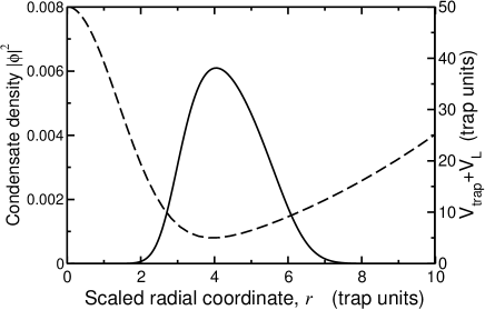
Figure 1: Torus potential (dashed line) and condensate density $\phi|^{2}$ (full line) as a function of radius in the the plane $z=0$. The radial potential corresponds to $h_{0}=50\hbar\omega_{r}$, and $\sigma=2\sqrt{\hbar/2m_{a}\omega_{r}}$. The condensate circulation is $\kappa=0$ and the interaction strength is $C=1000$. The scaled condensate probability density $|\phi|^{2}$ is given in units $({\hbar/2m_{a}\omega_{r}})^{3/2}$

II.2 Toroidal condensates

Conventional atom traps provide a confinement of the condensate in the radial and axial directions. We write this as a spheroidal potential of the type: $V={1\over 2}m_{a}\omega_{r}^{2}(r^{2}+\lambda^{2}z^{2})$, where $r$ is the radial coordinate, $\omega_{r}$ the radial frequency, and $z$ the axial coordinate. Here $\lambda$ is the aspect ratio of the harmonic potential, so that $\lambda>1$ flattens the condensate into an oblate pancake shape. For convenience we use scaled dimensionless units for length, time and energy namely: $(\hbar/2m_{a}\omega_{r})^{1\over 2},\omega_{r}^{-1}$ and $\hbar\omega_{r}$, respectively. Typically, $\omega_{r}\sim 2\pi\times 200$Hz, so that the natural timescale for oscillation is of the order of milliseconds. If this potential is supplemented by a repulsive core then the toroidal shape can be realized. The conventional method is to use blue-detuned laser light to create a dipole force. In the experiment of Davis et al. Davis et al. (1995) the AC Stark shift from the green light of an argon-ion laser ($\lambda=514$nm), detuned from the $D$-line ($\lambda=589$nm) of the trapped sodium atoms created the dipole force. If the laser beam is aligned along the $z$-axis of the trap at the diffraction limit focus then the potential if a function of $r$ only: $U(r)=\hbar I(r)(8\tau^{2}\ \Delta.I_{sat})^{-1}$, where $I_{sat}$ is the saturation intensity of the level, $\Delta$ is the detuning and $\tau$ the lifetime of the upper atomic level Adams and Riis (1997). Across the focus the intensity variation is Gaussian: $I(r)=I_{0}\exp(-r^{2}/\sigma^{2})$, where the on-axis intensity is related to the power $P$ and waist of the beam $w_{0}$ by $I_{0}=2P/\pi w_{0}^{2}$. So the width and height of the central barrier can be controlled by the these parameters. Consider a typical case for a trap containing sodium atoms; an argon-ion laser beam of 3.5 W focused to a waist $w_{0}=30\mu$m, would give a frequency shift of 7 MHz at $r=0$. Compared with trap frequencies of order $\omega_{r}/2\pi\sim 100-400$Hz, this would be sufficient to create a hole along the trap axis and form a toroidal condensate. The combination of the fields gives the external potential: $V_{\rm ext}({\bm{x}},0)={1\over 2}m_{a}\omega_{r}^{2}(r^{2}+\lambda^{2}z^{2})+h_{0}\exp(-r^{2}/\sigma^{2})$, where the repulsive central barrier is defined by height and width parameters $h_{0}$ and $\sigma$, respectively. The radial minimum of the well is displaced to $r_{0}=\sigma\sqrt{\ln(4h_{0}/\sigma^{2})}$. For convenience we use scaled dimensionless units for length, time and energy namely: $(\hbar/2m_{a}\omega_{r})^{1\over 2},\omega_{r}^{-1}$ and $\hbar\omega_{r}$, respectively Then it is convenient to define the interaction strength by the dimensionless parameter $C\equiv 8\pi N_{0}a_{s}(\hbar/2m_{a}\omega_{r})^{-{1\over 2}}$, so that as millions of atoms occupy the condensate $N_{0}\rightarrow\infty,C\rightarrow\infty$, while the ideal gas corresponds to $C\rightarrow 0$. For the pancake geometry $\lambda\gg 1$ the central barrier height $h_{0}$ controls the transition from spheroid to torus. The radius $r_{0}$ of the potential well minimum provides a guide to the size of the torus. Collective excitations for a quartic toroidal potential of the form: $V(r,z)_{\rm ext}={1\over 2}m_{a}\omega_{r}^{2}[(r-r_{0})^{2}+\lambda^{2}z^{2}]$ were considered by Salasnich et al Salasnich et al. (1999) and the variation in chemical potential and frequency with respect to particle number was studied. The geometry chosen Salasnich et al. (1999) was a prolate shape such that $\lambda=1/\sqrt{8}$ in contrast to the oblate case considered here. An example of a toroidal condensate density in static equilibrium is shown in figure 1. The trap parameters are $h_{0}=50\hbar\omega_{r}$, and $\sigma=2\sqrt{\hbar/2m_{a}\omega_{r}}$ so that $r_{0}\approx 4$, and the interaction strength is $C=1000$. For strong interaction, high $C$, the radius of gyration ($r_{K}$) about the symmetry axis is a better estimate of condensate radius; where $r_{K}^{2}\equiv\int|\phi|^{2}r^{2}d^{3}\bm{x}/\int|\phi|^{2}d^{3}\bm{x}$. For the pancake shape ($h_{0}=0$) $r_{K}=3.2$, but as the barrier is raised to $h_{0}=10$ then there is some depletion of condensate at the center, so that it expands to $r_{K}=3.8$. Finally for a high central barrier, $h_{0}=50$, the condensate is excluded from the trap axis and a narrow ring is formed with $r_{K}=4.6$ as shown in figure 1. Here the maximum condensate density is located close to the potential energy minimum $r_{0}\approx 4$ in accord with hydrostatic equilibrium Dalfovo et al. (1999).

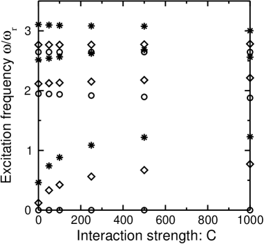
Figure 2: Excitation spectrum for the axisymmetric modes of semi-toroidal condensate without circulation ($\kappa=0$) as a function of interaction strength $C$. Trap parameters are $\lambda=\sqrt{7}$, $\sigma=2$. The symmetries of the modes are: $m=0\ (\circ)\$,$|m|=1\ (\diamond)\$, $|m|=2\ (\ast)\$.

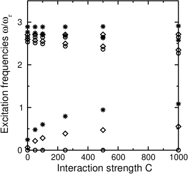
Figure 3: Excitation spectrum for the axisymmetric modes of toroidal condensate without circulation ($\kappa=0$) as a function of interaction strength $C$. Trap parameters are $\lambda=\sqrt{7}$, $\sigma=2$ and $h_{0}=50$. The mode symmetries are: $m=0\ (\circ)$,$|m|=1\ (\diamond)$, $|m|=2\ (\ast)$

II.3 Bogoliubov spectrum

In this paper we are primarily interested in the low-lying axisymmetric excitations arising from weak perturbation of the condensate, so that detailed results will be presented for the first few monopole, dipole and quadrupole excitations only. For finite $C$, the spectrum of excitations must be determined by numerical solution of equations (3,4) and (5). Separating variables gives:

$$\phi(r,z,\varphi)=\tilde{\phi}_{\kappa}(r,z)e^{i\kappa\varphi}$$ (6)

so that the condensate, with circulation $\kappa$ and real amplitude $\tilde{\phi}$, is the solution of the equation:

$${\cal{L}}_{(\kappa)}\tilde{\phi}_{\kappa}-g|\tilde{\phi}_{\kappa}|^{2}\tilde{\phi}_{\kappa}=0$$ (7)

where

$${\cal{L}}_{(s)}\equiv-{\displaystyle{\hbar^{2}\over 2m_{a}}\left({\partial^{2}\over\partial r^{2}}+\frac{1}{r}\frac{\partial}{\partial r}+\frac{\partial^{2}}{\partial z^{2}}-\frac{s^{2}}{r^{2}}\right)+}$$ (8)

$${\textstyle{1\over 2}}m_{a}\omega_{r}^{2}(r^{2}+\lambda^{2}z^{2})+h_{0}\exp(-r^{2}/\sigma^{2})+2g|\tilde{\phi}_{\kappa}|^{2}-\mu$$

The cylindrical symmetry of the condensate means that small amplitude excitations can be described by radial ($n_{r}$), axial ($n_{z}$) and rotational ($m$) quantum numbers, each with an associated parity. Here $m=n_{\theta}-\kappa=0,\pm 1,\pm 2,\dots$ denotes angular momentum with respect to the condensate, while $n_{r},n_{z}=0,1,2,3,\dots$. The quasiparticle amplitudes:

$$u_{n_{r},m,n_{z}}(r,z,\varphi)\equiv\tilde{u}_{n_{r},n_{z}}(r,z)e^{i(m+\kappa)\varphi}$$ (9)

$$v_{n_{r},m,n_{z}}(r,z,\varphi)\equiv\tilde{v}_{n_{r},n_{z}}(r,z)e^{i(m-\kappa)\varphi}$$ (10)

with corresponding angular frequency, $\omega_{n_{r},m,n_{z}}$, are solutions of the eigenvalue problem

$${\cal{L}}_{(m+\kappa)}\tilde{u}(r,z)+g\ \tilde{\phi}_{\kappa}^{2}\ \tilde{v}(r,z) = +\hbar\omega\tilde{u}(r,z)$$ (11)

$${\cal{L}}_{(m-\kappa)}\tilde{v}(r,z)+g\ \tilde{\phi}_{\kappa}^{2}\ \tilde{u}(r,z) = -\hbar\omega\tilde{v}(r,z)$$ (12)

The equations are discretised on a 2D-grid using Lagrange functions McPeake et al. (2002); the radial coordinate is defined at $M$ grid points ($r_{1},r_{2},\dots,r_{M}$) and the axial coordinate at $N$ points ($z_{1},z_{2},\dots,z_{N}$). Therefore:

$$\tilde{\phi}_{\kappa}(r,z)=\sum_{k=1}^{M}\sum_{l=1}^{N}\tilde{\phi}_{\kappa}^{kl}(r_{k},z_{l})\lambda_{k}^{-1/2}\mu_{l}^{-1/2}\ f_{k}(r)g_{l}(z)$$ (13)

where $f,g$ are Lagrangian interpolating functions such that

$$\int_{0}^{\infty}f_{i}^{\ast}(r)f_{k}(r)\ 2\pi r\ dr\approx\lambda_{i}\delta_{ik}$$ (14)

$$\int_{-\infty}^{\infty}g_{j}^{\ast}(z)g_{l}(z)\ dz\approx\mu_{j}\delta_{jl}$$ (15)

The functions for the $r$-coordinate are chosen to be generalized Laguerre polynomials McPeake et al. (2002), scaled to encompass the entire condensate, with typically $M=50$ mesh points. On the other hand, Hermite polynomials are used in the $z$-direction so that

$$g_{l}(z)=\sum_{l=0}^{N-1}\chi_{l}^{\ast}(z_{l})\chi_{l}(z)$$ (16)

where $\chi_{l}(z)=h_{N}^{-\frac{1}{2}}w(z)^{\frac{1}{2}}H_{l}(z)$. and $H_{l}(z)$ are the Hermite polynomials associated with weights $w(z)=e^{-z^{2}}$ and normalization factor $h_{N}=2^{N}\pi^{1/2}N!$. A high degree of accuracy was found with only $N=30$ points. The resultant eigenvalue problem was solved using the following approach. The condensate density was found using Newton’s method for equation (7). The decoupled linear eigenvalue problem (11,12) was solved by conversion to Hessenberg $QR$ form followed by inverse iteration Golub and van Loan (1996). Convergence was established by a combination of grid scaling and number of mesh points, so that at least six-figure precision was assured for all frequencies (see table 1 and table 2).

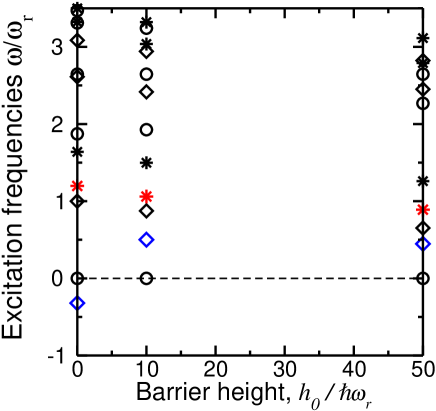
Figure 4: Excitation spectrum for modes of a condensate with circulation $\kappa=1$. The mode symmetries are $|m|=0(\circ),1(\diamond),2(\ast)$. Frequencies are plotted as a function of barrier height $h_{0}$ in a trap characterized by $\lambda=\sqrt{7}$ and $\sigma=2\sqrt{\hbar/2m_{a}\omega_{r}}$, with interaction strength $C=1000$. See also table 2

Table 1: Angular frequencies $\omega/\omega_{r}$ of the first-excited radial dipole modes. The table compares the numerical accuracy of the time-dependent linear response method (TDLR) with $\epsilon=0.02$ with the time-independent methods (BdG) and agreement is better than 2% in all cases. The condensate interaction strength is $C\equiv 8\pi N_{0}a_{s}(\hbar/2m_{a}\omega_{r})^{-{1\over 2}}=1000$ and the axial mode is $n_{z}=0$. Results are presented for $\kappa=0$ and $\kappa=1$.

	$h_{0}/\hbar\omega_{r}=10$		$h_{0}/\hbar\omega_{r}=50$
mode	TDLR	BdG	TDLR	BdG
$\kappa=0$
$m=+1$	0.772	0.771	0.563	0.554
$\kappa=0$
$m=-1$	0.772	0.771	0.563	0.554
$\kappa=1$
$m=+1$	0.875	0.874	0.657	0.652
$\kappa=1$
$m=-1$	0.496	0.501	0.448	0.447

Table 2: Excitation frequencies $\omega/\omega_{r}$ of the toroidal condensate with circulation $\kappa=1$ with variation in the central barrier height $h_{0}$. The condensate interaction strength is $C\equiv 8\pi N_{0}a_{s}(\hbar/2m_{a}\omega_{r})^{-{1\over 2}}=1000$

$m$	$h_{0}/\hbar\omega_{r}=0$	$h_{0}/\hbar\omega_{r}=10$	$h_{0}/\hbar\omega_{r}=50$
	2.646	2.646	2.646
	3.310	3.243	3.954
$m=0$	3.471	3.600	3.970
	4.691	4.480	4.771
	4.728	4.807	5.609
	4.936	5.027	5.882
	-0.320	0.501	0.447
$|m|=1$	1.000	0.875	0.652
	2.613	2.417	2.451
	3.085	2.942	2.823
	1.197	1.061	0.890
	1.640	1.498	1.260
$|m|=2$	3.499	3.037	2.790
	3.322	3.321	3.114
	4.925	4.530	4.396
	4.840	4.561	4.471

II.4 Spectrum of torus excitations

The Bogoliubov mode frequencies for a toroidal condensate without circulation ($\kappa=0$) are shown in figures  2 and  3 for two different barrier heights. The variation in frequencies as the particle number ($C$) increases is shown. In the absence of circulation for the low barrier $h_{0}=10$ (figure 2) the effect of increasing the interaction strength, or equivalently increasing the number of atoms in the condensate, is to spread the spectral lines of the low-lying modes, while the highly-excited state frequencies are relatively insensitive as $C$ increases. In contrast, to the prolate toroid results Salasnich et al. (1999) the effect of increasing atom number, increasing $C$,leads to an increase in the gap between the low-frequency excitations. The three $m=0$ modes shown are, in increasing frequency, the gapless mode $\omega=0$, the first breathing mode, and the first axial dipole mode $\omega=\sqrt{7}$. The lowest degenerate modes $m=\pm 1$ are the fundamental radial dipoles, at higher frequency $\omega\sim 2$ we observe an octupole mode, and finally the $xz$-quadrupole at $\omega\sim 2.8$ is very close to the axial dipole. The increasing density of states for higher excitations is familiar from studies of spherical condensates and is reproduced here. Finally the lowest pair of $m=2$ states, corresponding to quadrupole excitation in the radial coordinate are far below the next higher excitations of this symmetry.

As the toroidal shape is more sharply defined ($h_{0}=50$) the high-frequency modes become more tightly grouped (figure 2) and the gap to the lowest-order excitations widens. The long-wavelength low-energy modes are circulations around the torus, as shown in figure 3. The acoustic modes Dalfovo et al. (1999) appropriate in the limit $C\rightarrow\infty$, are sinusoidal oscillations in density $\delta\rho$ and follow the microscopic wave equation, in our units:

$$-\omega^{2}\delta\rho=2\nabla\cdot([\mu-V_{\rm ext}]\nabla\delta\rho)$$ (17)

In the Thomas-Fermi limit, the condensate occupies the region $\Omega$ where $\mu-V_{\rm ext}>0$. The angular waves satisfy the periodic boundary conditions $\delta\rho(\varphi+2\pi m)=\delta\rho(\varphi)$. Taking the volume average of equation (17) over the radial and axial density gives: $\omega=|m|\omega_{s}$ where

$$\omega_{s}^{2}\int_{\Omega}2\pi rdrdz=2C\int_{\Omega}r^{-2}\phi^{2}2\pi rdrdz$$ (18)

So that:

$$\omega=|m|\sqrt{2C\langle\phi^{2}r^{-2}\rangle}$$ (19)

The results in figure 2 reflect the change in dispersion relation $\omega\sim m^{2}$ to $\omega\sim m$ for the lower frequency modes as the interaction strength increases. The value of $\omega_{s}$ varies slowly with changes in the interaction strength $C$, see figure 3. It is worth noting that the simple formula (17) gives a good estimate of the frequency spectrum. For example, for $C=1000$ $\omega_{s}\approx 0.57$ in good agreement with the results shown (figure 3) while for $C=4300$ the value is $\omega_{s}\approx 0.78$. The relation (19) is quite general and can by applied to any toroidal geometry. For a large radius but tightly confined torus, so that $\langle r^{-2}\rangle\approx r_{K}^{-2}$ the relation simplifies to the 1D result as expected:

$$\omega=|m|\sqrt{2C/\Omega}\ r_{K}^{-1}$$ (20)

where the wavenumber is quantized according to $|m|/r_{K}$, and the speed of sound is proportional to the square root of the atom density. One might assume, for a given radial and axial mode, that this pattern of frequencies for the $m$ sublevels would be repeated for the higher frequency bands. In fact this is not the case as confirmed in figures 2 and 3. The bands become mixed and the $\omega\sim|m|$ relation does not hold. A more extensive list of the frequencies including the highly excited modes is given in Table 2.

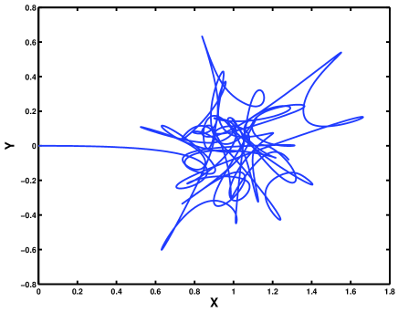
Figure 5: Center-of-mass trajectory of a toroidal condensate current $\kappa=1$ displaced from the trap center. The torus has parameters $\lambda=\sqrt{7}$, $\sigma=2\sqrt{\hbar/2m_{a}\omega_{r}}$ and $h_{0}=50\hbar\omega_{r}$ and interaction strength $C=1000$. The figure shows the path traced out over a total time $T=100$ in the horizontal plane by the condensate center-of-mass following a small horizontal displacement of the trap axis $\varepsilon=1$. The combination of the $x$-dipole and $y$-dipole oscillations leading to precession of the condensate. These dipoles modes are degenerate and nearly in phase. The spectrum density of the $x$-dipole oscillations is shown in figure 7

II.5 Toroidal current flow

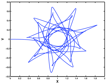
Figure 6: Center-of-mass trajectory of a toroidal condensate (current $\kappa=1$) after radial displacement. As in figure 5 the torus has parameters $\lambda=\sqrt{7}$, $\sigma=2\sqrt{\hbar/2m_{a}\omega_{r}}$ and $h_{0}=50\hbar\omega_{r}$, however the atom number is much higher in this case:$C=4300$. The figure shows the path traced out over a time $T=100$ in the horizontal plane by the condensate center-of-mass following a small horizontal displacement of the trap $\varepsilon=1$. The center of mass performs a circular motion due to two effects: the $x$ and $y$ dipole states are not degenerate in frequency and the amplitudes are out of phase, by roughly $\sim\pi/2$.

If the condensate itself has a current $\kappa\neq 0$, then the central barrier acts as a pinning site for the vortex. Furthermore the $\pm|m|$ degeneracy of the excitation modes is removed. Perturbations of the external potential are of interest since it allows us to study imperfections in the toroidal trap potential, and also the dissipation of the ring current. We propose that these modes can be studied by a lateral displacement of the trap. In Figure 4 the spectrum of excitations of a singly-quantized current loop $\kappa=1$ are presented. In this figure we consider the transition from a conventional pancake geometry $h_{0}=0$, through a semi-toroidal trap $h_{0}=10$, before reaching the torus shape $h_{0}=50$. The presence of the barrier creates a narrower radial well, so that the $m=0$ radial excitations are pushed to higher frequencies. The axial $m=0$ dipole mode $\omega=\lambda\approx 2.65$, is unaffected of course. The splitting of the $m$-degeneracy is greatest for the spheroidal $h_{0}=0$ case, in particular the lowest pair of $|m|=1$ modes. The co-rotating mode $m=+1$ has a positive frequency lying close to the lowest $m=2$ mode. The anomalous or counter-rotating mode $m=-1$ has a negative frequency, but positive norm. Anomalous modes arise when a condensate has a stable topological excitation such as a vortex, indeed the presence of a vortex is a necessary condition for an anomalous excitation as its presence is required to satisfy conservation of energy and momentum in the system Feder et al. (2001). In this case the central barrier raises the anomalous mode to positive frequencies effectively creating a stable pinning site for toroidal flow. The stability of high circulation current in toroidal traps has been discussed in detail by Busch et al. Busch et al. . The splitting of the $|m|=1$ pair reduces as the barrier rises and the condensate becomes toroidal. The closing of the energy gap reflects the fact that the barrier expels condensate density from the center so that the $m=-1$ cannot occupy the vortex core region and create a large energy gap. The $|m|=1$ modes will be evident when dipole excitations of the circulating flow are discussed. The $m=\pm 2$ states, degenerate in figure 3 , are also split by the condensate flow and in the toroidal limit, $h_{0}=50$. The energy splittings are proportional to $|m|$ the current momentum. This follows from the Bogoliubov equations when the centrifugal energy terms can be considered as perturbations. First-order perturbation theory applied to equations (11) and (12) gives the energy shift:

$$\Delta\hbar\omega\approx{\hbar^{2}(m+\kappa)^{2}\over 2m_{a}}(u_{0},r^{-2}u_{0})+{\hbar^{2}(m-\kappa)^{2}\over 2m_{a}}(v_{0},r^{-2}v_{0})$$ (21)

where $u_{0}$ and $v_{0}$ are the unperturbed quasiparticle states. This gives the energy splitting $\Delta E=\hbar(\omega_{+}-\omega_{-})$:

$$\Delta E\approx 4|m|\kappa\times{\hbar^{2}\over 2m_{a}}\int(u_{0}^{*}u_{0}-v_{0}^{*}v_{0})r^{-2}\ d^{3}{\bm{r}}$$ (22)

If the condensate and excitations are tightly confined around the radius $r_{K}$ then:

$$\Delta E\approx 4|m|\kappa\times{\hbar^{2}\over 2m_{a}r_{K}^{2}}$$ (23)

The splitting decreases as $C$, and hence $r_{K}$ increases. Referring to Table 1 for $h_{0}=50$, the $|m|=1$ splitting is close to that given by the perturbation expression (equation 23) $\Delta E\approx 0.19$. However the lowest $|m|=2$ modes in Table 1 have a splitting (0.37) very slighty smaller than the pertubation result $0.38$.

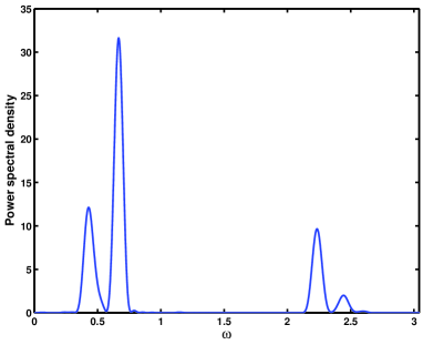
Figure 7: Spectral density of $x$-dipole of a condensate with circulation $\kappa=1$ corresponding to figure 5: $P_{x}\left(\omega\right)$ The torus parameters are $\lambda=\sqrt{7}$, $\sigma=2\sqrt{\hbar/2m_{a}\omega_{r}}$ and $h_{0}=50\hbar\omega_{r}$. The condensate interaction strength is $C=1000$ with trap displacement $\epsilon=1$. The figure shows the dominance of three modes, the low frequency $m=\pm 1$ doublet, and an excited $m=-1$ mode. The center of the doublet corresponds to the frequency $\omega_{s}=\sqrt{2C\langle r^{-2}\rangle}\approx 0.58$. In the graph the frequency peaks are shifted from the linear response results given in Table 1 and have a broader splitting than the Bogoliubov approximation. The $x$-dipole modes, shown above, have frequencies $\omega_{x}=0.421,0.666,2.237,2.441$ while the corresponding $y$-dipole modes have frequencies: $\omega_{y}=0.449,0.657,2.234,2.422$.

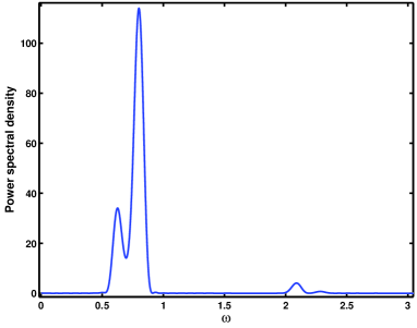
Figure 8: Spectral density of $x$-dipole of condensate with circulation $\kappa=1$ corresponding to figure 6: $P_{x}\left(\omega\right)$ The torus parameters are $\lambda=\sqrt{7}$, $\sigma=2\sqrt{\hbar/2m_{a}\omega_{r}}$ and $h_{0}=50\hbar\omega_{r}$. The condensate interaction strength is $C=4300$ with trap displacement $\epsilon=1$. The center of the doublet corresponds to the frequency $\omega_{s}=\sqrt{2C\langle\phi^{2}r^{-2}\rangle}\approx 0.78$ The figure shows the shifting upwards of the mode frequencies and a narrowing of the $m=\pm 1$ doublet splitting consistent with an expanded condensate with a higher sound speed. The modes shown above have frequencies: $\omega_{x}=0.625,0.804,2.095,2.284$. The corresponding $y$ dipole modes, not shown, have similar strengths but with frequencies $\omega_{y}=0.657,0.792,2.086,2.275$.

The simplest experimental scheme to observe these modes is to displace the potential in the horizontal plane and follow the motion of the condensate center-of-mass. Consider a sudden adjustment of the trapping potential

$$V_{\rm ext}\left(x,y,z\right)\rightarrow V_{\rm ext}\left(x-\varepsilon,y,z\right)$$ (24)

The effect on the center-of-mass is shown in figures 5 and figure 6 in which the trajectory is traced out as time evolves. These graphs were obtained by direct solution of the time-dependent Gross-Pitaevskii equation, following from taking arbitrary variation of $\psi^{*}$ in (1):

$$\left[H_{0}+g|\psi|^{2}-i\hbar\partial_{t}\right]\psi=0$$ (25)

For very small perturbations the nonlinearity is small and the time-dependent linear response method (TDLR) is equivalent to the stationary Bogoliubov equation method outlined above. This employs a direct numerical solution, in combination with spectral analysis can also be used to determine the frequency spectrum McPeake et al. (2002) and the strength of each frequency component, that is the population of modes and density fluctuations of the collective excitations. This can be done efficiently and accurately using spectral methods. The initial state can be determined by imposing the phase according to the value of $\kappa$ and evolving in imaginary time McPeake et al. (2002). The calculations presented here were performed on a $64\times 64\times 64$ grid. The scaling of grid spacing according to the degree of confinement ensures maximum spatial resolution of the condensate, so that the $z$ dimension is more tightly confined. The time step chosen, $\Delta t\approx 0.001\times 2\pi/\omega_{r}$, is dictated by the characteristic timescale of the excitations. A power-spectral-density estimate which used a Kaiser windowing function was employed to analyse the various moments of interest in terms of its component frequencies. For example the $x$-dipole moment can be transformed as follows:

$$P_{x}\left(\omega\right)=\left|\int_{0}^{T}e^{-i\omega t}\langle x\rangle dt\right|^{2}$$ (26)

The spectral data obtained for a very small trap displacement $\varepsilon=0.02$ confirms the mode frequencies from the Bogoliubov-de Gennes equation, and establishes the accuracy of the method. As shown in table 1, the frequencies using this method are accurate to within a few per cent. However a realistic measurement process based on density imaging requires a much larger amplitude motion in order to resolve the fluctuations. In this case, the nonlinear effect can be important. In our scheme, which we propose as a viable method to measure the spectrum, we consider the trap displaced by a substantial amount $\varepsilon=1$ in order to resolve the oscillations in the plane. When circulation of the toroidal current is disturbed in this manner the effect is to create large counter-circulating currents. If these currents are in phase and of equal magnitude the condensate would execute a pedulum motion. In general the motion will be 2D if the symmetry is broken. In terms of experimental observables, the effect appears as oscillations of the center of mass with a precessional motion. Similar precession motion for quadrupole excitation of a spheroidal vortex state has been noted McPeake et al. (2002). The locus of the center-of-mass in the horizontal plane from $t=0$ to $t=100$, is shown in figure 5 for $C=1000$ and $h_{0}/\hbar\omega_{0}=10$. Initially the condensate moves from $x=0,y=0$ towards the equilibrium point $x=1,y=0$, however this motion is converted an irregular precessing pendulum motion. The rate of precession is proportional to the splitting of levels. However the center-of-mass motion is not simple. A clearer understanding of the motion follows from a spectral analysis of the $x$ and $y$ dipole moments. In fact, the apparently irregular motion is dominated by only a few components the low frequency dipoles. In both the case $h_{0}=10$ (figure 7) and $h_{0}=50$ (figure 8) the $m=+1$ mode is stronger than the mode $m=-1$ and this dictates a motion with positive helicity, that is the condensate precession is in the same sense as the flow. However the frequencies are significantly different from the linear model and the $x$-$y$ degeneracy is removed due to the nonlinearity of the response in the $x$ direction. In figure 7, the torus parameters are $\lambda=\sqrt{7}$, $\sigma=2\sqrt{\hbar/2m_{a}\omega_{r}}$ and $h_{0}=50\hbar\omega_{r}$. The condensate interaction strength is $C=1000$ with trap displacement $\epsilon=1$. Comparing the $x$ frequencies with the values of table 1 we note the $y$-dipole frequencies are very similar in both cases, but the $x$-dipole pair splitting is increased when the trap displacement is this large. The motion shown in figure 5 is a superposition of a faster $x$ dipole with a slower $y$ dipole. The results for the higher interaction strength $C=4300$ show the splitting of the $|m|=1$ lines narrowing as the size of the condensate increases. The figure shows the shifting upwards of the mode frequencies and a narrowing of the $m=\pm 1$ doublet splitting consistent with an expanded condensate with a higher sound speed. The modes shown have frequencies: $\omega_{x}=0.625,0.804,2.095,2.284$. The corresponding $y$ dipole modes have similar strengths but with frequencies $\omega_{y}=0.657,0.792,2.086,2.275$. The nonlinear interactions give different splittings for the $x$ and $y$ dipoles: $\delta\omega_{x}=0.179$ compared with $\delta\omega_{y}=0.135$ both of which are slightly smaller than the linear perturbation theory (23) $\delta\omega\approx 0.200$. The major contrast between figures 5 and 6 is the orbiting motion observed for the higher value of $C$, although the frequency components shown in figures 7 and 8 are of similar relative strengths, the $x$ and $y$ dipoles have a large phase difference close to $\pi/2$ for $C=4300$ and explains the more circular character of the motion. This is slightly surprising in that the usual behavior of collective mode of oscillations is that the frequency dependence on $N$ is relatively weak for large $N$. In this respect, collective excitation frequencies are usually a poor method of estimating condensate fraction compared with the hydrostatic pressure. However, in this case the toroidal geometry seems to retain the quantum features of the excitations even for large particle number.

III Conclusions

In this paper we studied the spectrum of collective excitations of oblate toroidal condensates within the Bogoliubov approximation, and explored the dynamical stability of ring currents around the torus. The main features we noted are generic to this design of trap and would apply to similar geometries and would be exhibited in experiments on toroidal condensates. The transition from spheroidal to toroidal geometry of the trap displaces the energy levels into narrow bands. The lowest-order modes are quasi one-dimensional circulations with dispersion relation $\omega\sim m\omega_{s}$ with $m$ quantized. When the condensate has an toroidal current flow, the low-energy circulations are split into co-rotating and counter-rotating pairs. A simple, but accurate, formula is presented for the lowest angular acoustic modes of excitation, and the splitting energy when a background current is present. The stability of the flow is maintained by the central barrier acting as a pinning site.

Instabilities will most readily occur by radial dipole excitations. The dipole states are nearly degenerate in the toroidal limit. Small condensate currents when disturbed create slow precessional motion through the center of the trap through mixing of the degenerate $x$ and $y$ dipole states. For a tightly confined torus, these modes are well separated in energy and accessible to observation. We propose an experiment that would detect these modes. A realistic measurement requires resolution of the global condensate motion. Large displacements, such as those we propose, give rise to small nonlinear shifts in the frequencies beyond the Bogoliubov model. We also note that the highly occupied condensate performs a circular orbiting motion of the center-of-mass. Such features are resolvable and experimentally measurable with current technology and expertise.

References

- Penckwitt and Ballagh (2001) A. A. Penckwitt and R. J. Ballagh, J. Phys. B: At. Mol. Opt. Phys. 34, 1523 (2001).
- Hutchinson and Zaremba (1998) D. W. Hutchinson and E. Zaremba, Phys. Rev. A 57, 1280 (1998).
- (3) D. S. Rokhsar, eprint cond-mat/9709212.
- Salasnich et al. (1999) L. Salasnich, A. Parola, and L. Reatto, Phys. Rev. A 59, 2990 (1999).
- Benakli et al. (1999) M. Benakli, S. Raghavan, A. Smerzi, S. Fantoni, and S. R. Shenov, Europhys. Lett. 46, 275 (1999).
- Arnold and Riis (2002) A. S. Arnold and E. Riis, J. Mod. Opt. 49, 959 (2002).
- Crompvoets et al. (2001) F. M. Crompvoets, H. L. Bethlem, R. T. Jongma, and G. Meijer, Nature 411, 174 (2001).
- Drummond et al. (2001) P. D. Drummond, A. Eleftheriou, K. Huang, and K. V. Kheruntsyan, Phys. Rev. A 63, 053602 (2001).
- Garay et al. (2001) L. J. Garay, J. R. Anglin, J. I. Cirac, and P. Zoller, Phys. Rev. A 63, 023611 (2001).
- Brand and Reinhardt (2001) J. Brand and W. P. Reinhardt, J. Phys. B: At. Mol. Opt. Phys. 34, L113 (2001).
- Petrov et al. (2000) D. S. Petrov, G. V. Shlyapnikov, and J. T. M. Walraven, Phys. Rev. Lett. 85, 3745 (2000).
- Girardeau and Wright (2001) M. D. Girardeau and E. M. Wright, Phys. Rev. Lett. 87, 210401 (2001).
- Davis et al. (1995) K. B. Davis, M. O. Mewes, M. R. Andrews, N. J. van Drutten, D. S. Durfree, D. M. Kurn, and W. Ketterle, Phys. Rev. Lett. 75, 3969 (1995).
- Matthews et al. (1999) M. R. Matthews, B. P. Anderson, P. Haljan, D. S. Hall, C. E. Wieman, and E. A. Cornell, Phys. Rev. Lett. 83, 2498 (1999).
- (15) T. Busch, J. Anglin, and W. Zurek, eprint cond-mat/0103394.
- Schulte et al. (2002) T. Schulte, L. Santos, A. Sanpera, and M. Lewenstein, Phys. Rev. A 66, 033602 (2002).
- McPeake et al. (2002) D. McPeake, H. Nilsen, and J. F. McCann, Phys. Rev. A 65, 063601 (2002).
- Nilsen et al. (2003) H. Nilsen, D. McPeake, and J. F. McCann, J. Phys. B: At. Mol. Opt. Phys. 36, 1703 (2003).
- Adams and Riis (1997) C. S. Adams and E. Riis, Prog. Quantum Elect. 21, 1 (1997).
- Dalfovo et al. (1999) F. Dalfovo, S. Giorgini, L. P. Pitaevskii, and S. Stringari, Rev. Mod. Phys. 71, 463 (1999).
- Golub and van Loan (1996) G. H. Golub and C. F. van Loan, Matrix Computations (Johns Hopkins University Press, 1996).
- Feder et al. (2001) D. L. Feder, A. A. Svidzinsky, A. L. Fetter, and C. W. Clark, Phys. Rev. Lett. 86, 564 (2001).