Voronoi and Fractal Complex Networks and Their Characterization

Abstract

Real complex networks are often characterized by spatial constraints such as the relative position and adjacency of nodes. The present work describes how Voronoi tessellations of the space where the network is embedded provide not only a natural means for relating such networks with metric spaces, but also a natural means for obtaining fractal complex networks. A series of comprehensive measurements closely related to spatial aspects of these networks is proposed, which includes the effective length, adjacency, as well as the fractal dimension of the network in terms of the spatial scales defined by successive shortest paths starting from a specific node. The potential of such features is illustrated with respect to the random, small-world, scale-free and fractal network models.

Several natural objects and phenomena can be modeled in terms of networks of basic components intensively exchanging information between themselves. Recent findings about the behavior of real networks, noticeably the small-world and scale-free modelsAlbert and Barabási (2002), motivated a renewal of interest in mathematical and statistical investigations of the properties of such complex structures. These studies often consist of estimating fundamental properties of the network, such as the degree distribution, clustering coefficient, and average length, for several network parameter configurations. For instance, the degree distribution of networks where the probability of new connections is proportional to the node degree has been verified to follow a power law Albert and Barabási (2002), indicating scale invariance, hence the name scale-free networks. While such investigations have led to a series of interesting findings, relatively little attention, with a few exceptions Waxman (1988); Manna and Kabakcioglu (2003), has been given to the role of spatial relationships between the network nodes as constrains to the network topology. Indeed, connections in real networks are often inherently related to the spatial positions of the constituent nodes as well as to their spatial adjacencies. Real networks falling into this category include but are not limited to telephone and electric power distribution, transportation systems, computer networks, spatio-temporal gene activation in animal development, as well as the neuronal networks in the mammals retina and cortex.

The following three main kinds of spatial requirements are considered here: (i) connect adjacent or near nodes, (ii) minimize the access (according to some cost such as time or distance) to more distant regions of the net and (iii) minimize the number and/or total length of edges. As such items are often incompatible – e.g. minimizing the access between any pair of nodes implies a large number of edges, networks are often characterized by a compromise between such requirements. One of the purposes of the current work is to investigate how the topologies of complex networks are related to spatial constraints. In other words, as the topology of real networks is often optimized to suit specific tasks, it becomes particularly important to obtain measurements directly expressing such spatial/function relationships.

Traditional random, small-world and scale free networks, as well as fractal networks, are considered in this paper. The network nodes are assumed to be spatially distributed along the two-dimensional region $\Omega$ according to the Poisson distribution with parameter $p$. The domain $\Omega\subset R^{2}$ where the network is embedded is assumed to be the square $(0\leq x\leq L,0\leq y\leq L)$. The Euclidean distance between any two nodes $i$ and $j$ is represented as $d_{i,j}$. Each point $(x,y)$ of $\Omega$ is associated to the nearest network node, which defines a Voronoi partition of $\Omega$ Ahuja and Schachter (1983), and consequently a Voronoi network. The spatial position of each network node $i$, $i=1,2,\ldots,N$, is expressed as $P_{i}=(x_{i},y_{i})$, and the area of the Voronoi cell respectively associated to this point is henceforth represented as $A_{i}$. Given the initial nodes, any type of network can be constructed by adding connections between them. The degree of a specific node $i$ is $k_{i}$, and the cost (or length) of the edge between nodes $i$ and $j$, hence $\lambda_{i,j}$, is given by the Euclidean distance between those nodes. As the networks considered here are not oriented, we have that $\lambda_{i,j}=\lambda_{j,i}$. Infinite length is assigned to inexistent edges and not taken into account for the statistics. The shortest path between two nodes $i$ and $j$, expressed as $\varepsilon_{i,j}$, is given by the sum of the edge lengths composing that shortest path.

The concept of hierarchy provides a powerful organizational framework to model several real networks Dorogovtsev et al. (2002); Barabási et al. (2004); Ravasz and Barabási (2003). Such a structuring can be immediately extended to Voronoi networks. Indeed, the tessellation of the network space $\Omega$ provides a natural and generic basis for defining a broad class of spatially constrained hierarchical and fractal networks. The basic construction principle is to define a new network inside each of the current Voronoi cells, as illustrated in Figure 1. Each added hierarchy is identified by successive integer indices $t=0,1,\ldots,Q$, and it is henceforth assumed that the nodes can only make connections inside their respective Voronoi cell and with the parent node, to which they are connected according to some statistical role, e.g. obeying uniform distribution with fixed parameter $\gamma_{m}$, as adopted henceforth. At least one random connection is guaranteed between the parent cell and one of the nodes of the daughter cell. In this way, the overall network can be understood as a series of spatially congruent networks connected along the hierarchical levels. The parameter $\gamma_{m}$ controls the level of interaction between distinct hierarchies. In case $\gamma_{m}$ is low, the subnetworks behave in an almost independent fashion. A broad variety of connecting models can be adopted inside each Voronoi cell, including random, small-world and scale-free approaches. Although hybrid networks can be obtained by using different connecting schemes at each hierarchical level or cell, the fractal networks in this article are all homogeneous and random.

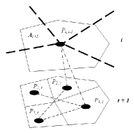
Figure 1: A Voronoi cell defined by node $P_{i,t-1}$ at hierarchy $t$ and a daughter network and respective Voronoi partition at the subsequent hierarchical level. 

Different fractal networks can be obtained by varying the nodes distribution inside each cell and the way in which the connections between the nodes are established. It is henceforth assumed that each Voronoi cell along the hierarchies have the same average number of nodes $M$ throughout, so that the average total number of nodes at level $t$ is $M^{t+1}$. Since $M$ is maintained throughout the network, cells at subsequent hierarchies become progressively denser, implying smaller spatial scale and increased level of details. The connections at any hierarchical level are uniformly established with the same probability $\gamma$, and it is reasonable to make $\gamma=\gamma_{m}$. The network starts from hierarchy $t=0$ with the $M$ nodes being connected with probability $\gamma_{m}$ to the initial master node $P_{0}$. As the distribution of points inside each cell at level $t$ obeys a Poisson distribution with parameter $p_{t}$, we have $M=p_{t}\left<A_{t}\right>$ and $\left<A_{t}\right>=1/(p_{t-1})$ Ahuja and Schachter (1983), so that $p_{t}=p_{t-1}M=p_{0}M^{t}$. Observe that $A_{0}=L^{2}$. The tessellations extend up to hierarchy $t=Q$ such as $p_{Q}<1$. Therefore $Q<-log(p_{0}-M)$. The average total number of nodes at level $t$ is $N_{t}=p_{t}A_{0}$, so that the average total amount of nodes in the network is $N=1+\sum_{t=0}^{Q}p_{t}A_{0}$. The average node degree at any cell in hierarchy $t$ is $\left<k_{t}\right>\cong\gamma M$. The characteristics of the network are therefore completely determined by the choice of $L$, $\gamma$, $M$ and $p_{0}$.

The self-similar nature of such fractal random networks, allied to the fact that several of the properties inside each cell is independent of those in other cells, allow convenient estimation of many network features. In case the distribution of a measurement $w$ inside any cell at any cell in level $t$ can be expressed in terms of $t$, i.e. $P_{t}(w)$, it is possible to estimate its distribution from level $0$ to $b<Q$ by using Equation 1.

$$P(w)=\frac{1}{\sum_{t=0}^{b}c_{t}}\sum_{t=0}^{b}c_{t}P_{t}(w)$$ (1)

where $\left<c_{t}\right>=A_{0}p_{0}M^{t-1}$ is the average number of Voronoi cells at level $t$. In case $P_{t}(w)$ is constant with respect to $t$ and not too dispersed, as can be the case with $\left<n_{t}\right>$ and $\left<k_{t}\right>$ under certain circumstances Albert and Barabási (2002), the resulting distribution will lead to the same distribution $P_{t}(w)$, now more intensely sampled. For instance, in the case of fractal random networks, we have that the degree distribution for $N$ nodes will approach that of a random network with $M$ nodes. In other words, the degree distribution of the fractal network does not follow a power law and is smaller than for a random network with the same overall number of nodes. The characteristic spatial scale at level $t$, hence $r_{t}$, can be defined as the radius of the equivalent circle with area $A_{t}$. Consequently, $r_{t}=(\pi p_{0})^{-0.5}M^{0.5(1-t)}$. Any network property directly proportional to $r_{t}$, as is the case with the edge length, shortest path and nearest neighbor distances, will therefore follow a power law along $t$ with exponent $-0.5log(M)$. Such a property will also be characterized by unit fractal dimension with respect to $s_{t}=log(r_{t})$.

The following measurements are suggested and used in the present work to characterize the spatial properties of complex networks in a more complete fashion:

Edge distance: Although the average length, meaning the average shortest path between any two network nodes, has been traditionally used in order to characterize complex networks Albert and Barabási (2002), the distribution of the Euclidean distances between two directly connected nodes $i$ and $j$ can also be provide useful information about the spatial characteristics of the network. The edge distance is henceforth expressed as $\lambda_{i,j}$, with average $\left<\lambda\right>$.

Effective distance: This feature applies to each pair of nodes $i$ and $j$, defined as the sum $S$ of the Euclidean distances of the edges composing the shortest path between those nodes, in case it exists, and the Euclidean distance between them, i.e. $E_{i,j}=S/\lambda_{i,j}$. Its maximum value of 1 is achieved whenever the shortest path equals the Euclidean distance, implying that all edges are parallel to the edge between $i$ and $j$. Large values of $E_{i,j}$ indicate network adherence to criterion (ii).

Adjacency: This measurement, represented as $\alpha_{i}$, is defined for each node $i$ as the number of direct connections it establishes with its $n_{adj}$ spatially adjacent neighbors divided by $n_{adj}$. Thus $0\leq\alpha_{i}\leq 1$. Although slightly similar to the clustering coefficient (e.g. Albert and Barabási (2002)), this feature differs in the sense that it takes the spatial adjacency explicitly into account. The average of this feature for all network nodes, i.e. $\left<\alpha\right>$, can be used to quantify criterion (i).

Network fractal dimension: While the average length and network diameter Albert and Barabási (2002) have been traditionally applied to quantify the edges length distribution along the network, we present an additional measurement, related to the multiscale spatial dimension Barbosa et al. (2003), which is capable of expressing the self-similarity/fractality of the network as the shortest distance nodes are found while the network is inundated (or visited) starting from any specific node $i$. The network fractal dimension, therefore, is a function of the spatial scale $s=log($Euclidean distance$)$, defined for each node $i$ and represented as $f_{i}(s)$. First, the sorted sequence ${p_{i,1},\ldots,p_{i,j},\ldots,p_{i,N}}$ of shortest paths (considering the Euclidean distance and not the number of nodes) between $i$ and every other node $j$ in the network is obtained by using traditional methods. The area distribution of node $i$ can now be defined as $h_{i}(s)=\sum_{j=0}^{N}A_{i}\delta(s-log(p_{i,j}))$, where $\delta$ is Dirac’s delta function. The cumulative distribution of areas is given as $\Theta_{i}(s)=\int_{-\infty}^{s}h_{i}(w)dw$. In order to obtain an interpolated and smoothed version of $\Theta_{i}(s)$, this function is convolved with a regularizing Gaussian kernel yielding $B_{i}(s)=\Theta_{i}(s)*g_{\sigma}(s)$, where $g_{\sigma}$ is the normal distribution with standard deviation $\sigma$ and $*$ stands for the convolution operation. Now, by making $H_{i}(s)=log(B_{i}(s))$, the fractal dimension of node $i$ as an adimensional function of the spatial scale is given by Equation 2.

$$f_{i}(s)=d\,H_{i}(s)/ds=B^{\prime}_{i}(s)/B_{i}(s)$$ (2)

The higher the value of $f_{i}(s)$, the faster the accumulated area increases along the subsequent shortest paths at the respective spatial scale $s$. Given that the areas of the Voronoi cells are added at once whenever their respective distances are reached, fractal dimensions larger than 2 can be observed. Similarly, the adoption of edge costs smaller than the respective Euclidean distance also leads to ‘superfractal’ dimensions, in the sense that its dynamics while it undergoes inundation exceeds the topological dimension of the space where the network is embedded. Observe that it is also possible to obtain fractal dimensions starting from a set of points instead of a single point. Figure 2 shows a node spatial distribution (a), the area distribution obtained from the respective Voronoi tessellation (b), the cumulative distribution (c) and the fractal dimension (d), all in terms of the spatial scale $s$. Such results were obtained by starting the network inundation from the leftmost point in (a). While each local minimum of $f_{i}(s)$ identifies a bottleneck along the network topology, as clearly illustrated in this example, the average fractal value $\left<f\right>$ taken along all possible scales provides an interesting quantification of the overall spatial connectivity of the nodes in the net.

The four diagrams in Figure 3 show the distribution of the above suggested measurements, taken pairwise, experimentally obtained from several realizations of each network model considering $L=121$ and $\gamma=0.02$. For comparison’s sake, all simulations had number of edges as close as possible to $n=350$, as well as number of nodes $N\cong 140$. In the case of the fractal random network, we used $M=5$, $p_{0}=0.00035$ and $\gamma=0.5$. For Watts-Strogatz, $p=10\gamma$, with the initial configuration obtained by directly connecting all spatially adjacent nodes. The Albert-Barabási model used $m_{0}=10$ and $m=3$, and $M=5$ and $p_{0}=0.000034$ were adopted for the fractal random networks. Distinctively segregated clusters were obtained in most cases, except for (d), and the fractal random measurements resulted generally more dispersed than those obtained for the other models. This is a consequence of the relatively low number of nodes $M=5$ required in order that the total number of network nodes results similar to those of the other simulated models.

From figure 3(a) we have that the fractal random network led to the highest overall cluster coefficients $C$ and average lengths $\ell$ values. The adjacencies in (b) increase along the following sequence: Albert-Barabási, random, fractal random and Watts-Strogatz. The distinctively high adjacency values and low shortest distance values exhibited by the Watts-Strogatz model is a direct consequence of the initial adjacent configuration used in that case. The more intense spatial regularity of that model also led to high effective length values and low edge distances in the phase space in (c), which is also marked by low dispersion of the average edge distances. The fractal random network yielded effective distances slightly higher than those obtained for the Albert-Barabási network, which was also characterized by small edge distances, which reflects the larger number of small spatial scale Voronoi cells. Indeed, the spatially adjacent and spatially uniformly distributed connections in the Watts-Strogatz case also implied most measurements to be less dispersed. As shown in (d), the random and Albert-Barabási networks behave similarly with respect to average fractal dimension and node degree, whose values are the highest among the considered network models. The fractal random network led to the smallest node degrees and intermediate fractal dimensions. The spatially more localized connections in the Watts-Strogatz network, makes its inundation smoother, implying the lowest fractal dimension values. Except for this network, a positive correlation is observed in (d), reflecting the fact that higher node degrees tends to favor higher fractal dimensions. Another interesting point in (d) is that the less spatially localized connections in the random and Albert-Barabási networks induced superfractal behavior. As a matter of fact, the relatively smaller average fractal dimensions presented by the Watts-Strogatz and fractal random models can be taken as an indication that they are more intensely influenced by spatial constraints, as is indeed the case.

The above results illustrate the potential of the suggested network measurements for quantifying and analysing the properties of networks as far as the possible influence of spatial constraints are concerned, providing a comprehensive integrated framework for investigating real complex networks. Of particular interest are the local/global hierarchical and topographical organization of mammals’ cortical structures, the relationship between neuronal function and connectivity and shape da F. Costa et al. (2003), as well as the spatio-temporal gene activation patterns underlying animal development. Other interesting possibilities are to consider fractal networks where the subsequent partition of the Voronoi is done with probability reflecting the degree of the parent node and/or additional spatial constraints such as varying density along $\Omega$.

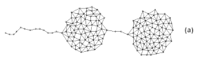
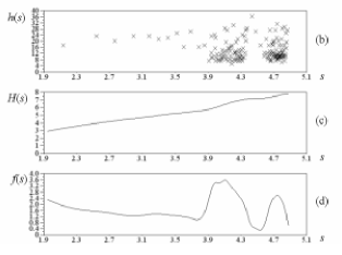
Figure 2: A Voronoi network (a) and its respective area distribution (b), logarithm of cumulative areas (c) and fractal dimension in terms of the spatial scale $s$ (d). 

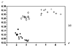
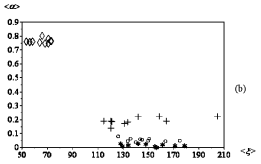
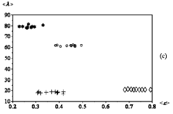
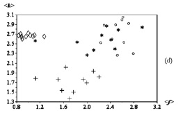
Figure 3: Phase space distributions of pairs of average measurements obtained from several realizations of the considered network models (random = $\circ$, Watts-Strogatz = $\diamond$, Albert-Barabási = $\star$ and fractal random = $+$).

References

- Albert and Barabási (2002) R. Albert and A. L. Barabási, Rev. Mod. Phys. 74, 47 (2002).
- Manna and Kabakcioglu (2003) S. S. Manna and A. Kabakcioglu, cond-mat 2, 0302224 (2003).
- Waxman (1988) B. Waxman, IEEE J. Selec. Areas Commun. SAC–6, 1617 (1988).
- Ahuja and Schachter (1983) N. Ahuja and B. J. Schachter, Pattern Models (John Wiley and Sons, New York, 1983).
- Barabási et al. (2004) A. Barabási, Z. Dezsö, E. Ravasz, S.-H. Yook, and Z. Oltvai (2004), to appear in Sitges Proceedings on Complex Networks, 2004.
- Dorogovtsev et al. (2002) S. N. Dorogovtsev, A. V. Goltsev, and J. F. F. Mendes, Phys. Rev. E 65, 066122 (2002).
- Ravasz and Barabási (2003) E. Ravasz and A. Barabási, Phys. Rev. E (2003), in print.
- Barbosa et al. (2003) M. S. Barbosa, L. da F. Costa, and E. de S. Bernardes, Phys. Rev. E (2003), in press.
- da F. Costa et al. (2003) L. da F. Costa, M. S. Barbosa, V. Coupez, and D. Stauffer, Brain and Mind (2003), in press.