Universality of the Lyapunov regime for the Loschmidt echo

Abstract

The Loschmidt echo (LE) is a magnitude that measures the sensitivity of quantum dynamics to perturbations in the Hamiltonian. For a certain regime of the parameters, the LE decays exponentially with a rate given by the Lyapunov exponent of the underlying classically chaotic system. We develop a semiclassical theory, supported by numerical results in a Lorentz gas model, which allows us to establish and characterize the universality of this Lyapunov regime. In particular, the universality is evidenced by the semiclassical limit of the Fermi wavelength going to zero, the behavior for times longer than Ehrenfest time, the insensitivity with respect to the form of the perturbation and the behavior of individual (non-averaged) initial conditions. Finally, by elaborating a semiclassical approximation to the Wigner function, we are able to distinguish between classical and quantum origin for the different terms of the LE. This approach renders an understanding for the persistence of the Lyapunov regime after the Ehrenfest time, as well as a reinterpretation of our results in terms of the quantum–classical transition.

I
Introduction

Controlling the phase in the evolution of a quantum system is a fundamental problem that is becoming increasingly relevant in many areas of physics. In relatively simple systems, like a quantum dot in an Aharanov-Bohm ringcit-HeiblumNature , the phase can even be measured by transport experiments. The development of the quantum information field requires the control of the phase of increasingly complex systemscit-DiVincenzoNature . Such a control is hindered by interactions with the environment in a way which is not completely understood at present.

Nuclear Magnetic Resonance provides a privileged framework to test our ideas on the evolution and degradation of the quantum phase. The phenomenon of spin echo, through the reversal of the time evolution, allows to study how an individual spin, in an ensemble, loses its phase memorycit-HannEcho . The randomization of its phase appears as a consequence of the interaction with other spins that act as an environment. Recently, it has become possible to test the phase of the collective many-spin state through the experiments of Magiccit-Pines and Polarizationcit-Polecho echoes. In these cases a local polarization “diffuses” away as consequence of the spin-spin interactions in the effective Hamiltonian $\mathcal{H}$. The whole many-body dynamics is then reversed by the sudden transformation $\mathcal{H}\rightarrow-\mathcal{H}$ . However, there is an increasing failure to reach the initial polarization state which is a consequence of the fluctuations of the phase of the complex quantum statecit-JChemPhys and is a measure of the entropy growthcit-MolPhysics .

Surprisingly, the rate of loss of information of the phase appears as an intrinsic property of the system, being quite insensitive to how small is the coupling to the external degrees of freedom or the precision of the reversalcit-Potencia . This may be interpreted as analogous to the residual resistivity of impure metals. When the direct coupling to the thermal bath is decreased by lowering the temperature, the resistivity becomes controlled by the reversible elastic scattering with impurities cit-Zeeman ; cit-Laughlin . The common feature of both intrinsic behaviors is the complexity of the dynamics that justifies the stosszahlansatz or molecular chaos hypothesis.

However, such an hypothesis does not seem to be compatible with our basic knowledge of quantum dynamics. Unlike classical mechanics, quantum dynamics exhibits a remarkable insensitivity to initial conditions cit-QChaos-europ ; cit-Haake . That is why the field known as quantum chaos deals mainly with the quantum stationary properties of systems whose underlying classical dynamics is chaotic. Among these properties, the ones more frequently studied are the level statisticscit-Bohigas , wave function scarring cit-scars , and parametric correlations cit-Aaron . A notable exception among these studies was that of Peres cit-Peres , who realized that classically chaotic and integrable systems behave differently under imperfect time reversal, for very short and long times. It is through the experimental findings above cited, that the study of time evolution of classically chaotic systems has gained a privileged place in nowadays research.

A simplified version of the echoes experimentally studied is the so-called Loschmidt echo (LE)

$$M(t)=\left|m(t)\right|^{2}=\left|\left\langle\psi_{0}\right|e^{\mathrm{i}(\mathcal{H}_{0}+\Sigma)t/\hbar}\ e^{-\mathrm{i}\mathcal{H}_{0}t/\hbar}\left|\psi_{0}\right\rangle\right|^{2},$$ (1)

where $\left|\psi_{0}\right\rangle$ is an arbitrary initial state that evolves forward in time under the system Hamiltonian $\mathcal{H}_{0}$ for a time $t$, and then backwards under a slightly perturbed Hamiltonian $\mathcal{H}_{0}+\Sigma$. The amplitude $m(t)$ of the LE is the overlap between the two slightly different evolutions of the same initial state, and $M(t)$ quantifies the departure from the perfect overlap. Because of this important property, within the field of Quantum Information the LE is referred to as “fidelity” Chuang . Alternatively, $M(t)$ can also be written as the trace of the product of two pure-state density matrices $\rho$ or Wigner functions $W$ evolving with different Hamiltonians,

$$M(t)=\mathop{\rm tr}\{\rho_{\mathcal{H}_{0}+\Sigma}(t)\ \rho_{\mathcal{H}_{0}}(t)\}=(2\pi\hbar)^{d}\int\mathrm{d}\mathbf{r}\int\mathrm{d}\mathbf{p}\ W_{\mathcal{H}_{0}+\Sigma}(\mathbf{r},\mathbf{p};t)\ W_{\mathcal{H}_{0}}(\mathbf{r},\mathbf{p};t)\ .$$ (2)

We have used the standard definitions

$$\rho_{\mathcal{H}}=\left|\psi\right\rangle\left\langle\psi\right|\ ,\ \text{with}\ \left|\psi\right\rangle=e^{-\mathrm{i}\mathcal{H}t/\hbar}\left|\psi_{0}\right\rangle,$$ (3)

$$W_{\mathcal{H}}(\mathbf{r},\mathbf{p};t)=\frac{1}{(2\pi\hbar)^{d}}\int\mathrm{d}\delta\mathbf{r}\ \exp{\left[-\frac{\mathrm{i}}{\hbar}\ \mathbf{p}\cdot\delta\mathbf{r}\right]}\ \left\langle\mathbf{r}+\frac{\delta\mathbf{r}}{2}\right|\rho_{\mathcal{H}}\left|\mathbf{r}-\frac{\delta\mathbf{r}}{2}\right\rangle,$$ (4)

where $d$ is the dimensionality of the space.

In consistency with the experimental behavior of the polarization echo, the LE of a classically chaotic one-body Hamiltonian $\mathcal{H}_{0}$ was found to exhibit an intrinsic decay rate cit-Jalabert-Past . This result is valid beyond some critical value of the perturbation. Interestingly, the decay rate is precisely the Lyapunov exponent $\lambda$ of the classical system. A related relevance of the classical dynamics had been hinted from the analysis of the entropy growth of dissipative systems cit-Zurek-Paz .

The purely Hamiltonian character of the model of Ref. cit-Jalabert-Past, , as well as the result of a classical parameter ($\lambda$) governing a bona fide quantum property ($M$), attracted considerable attention. A quite intense activity has been devoted in the last two years in order to test these predictions in various model systems and pursue further developments of the theory cit-PhysicaA ^-cit-Mirlin .

The Lyapunov behavior has been numerically obtained in models of a Lorentz gas cit-Lorentzgas , kicked topscit-Jacquod01 ; cit-WangLi , Bunimovich stadium cit-Bunimovich , bath tube stadium cit-SmoothBilliard and sawtooth map cit-BenentiCasati . The analytical results have been mainly focused in the small perturbation region. Jacquod and collaborators cit-Jacquod01 identified the regime below the critical perturbation as following a Fermi Golden Rule through the energy uncertainty produced by the perturbation which were also analyzed with semiclassical tools cit-CerrutiTomsovic . Prosen and collaborators cit-Prosen ; cit-ProsenSeligman showed that $M(t)$ in the perturbative regime depends on the specific time dependence of the perturbation correlation functions.

The Lyapunov regime bears a clear signature of the underlying classical dynamics. This observation lead Benenti and Casati cit-BenentiCasati to propose that the independence of the decay rate on the perturbation strength is a consequence of the quantum-classical correspondence principle. As we will analyze in this work, the situation is far less trivial. We are going to show that this regime persists for times much larger than the Ehrenfest time (as defined by Berman and Zavslavsky cit-BermanZavslasky ). In addition, the quantum LE is functionally different than what a direct estimation would yield for the classical LE (for the chaotic cit-Jalabert-Past , as well as the integrable cit-JacquodInt cases). Moreover, the classical counterpart of the LE is problematic since a wide range of dynamic behaviors is obtained in different situations cit-Eckart ; cit-CasatiClassic .

The LE has also been studied in different disordered systems cit-PhysicaA ; cit-Mirlin . It has been shown in both cases that the long range of the perturbing potential, as emphasized in Ref. cit-Jalabert-Past, , is crucial in order to obtain a perturbation independent regime.

The various approximations that the semiclassical theory of Ref. cit-Jalabert-Past, relies on were further corroborated using an initial momentum representation of the wave–packet Heller . This changes the sum over an uncontrolled number of trajectories into only one, which allows the exact numerical evaluation of the semiclassical expression for the echo.

Taking the perturbation as the action of an external environment allows us to think of the LE as a measure of the decoherence. This approach has been advocated by Zurekcit-ZurekNature , and extendedcit-LESubPlanck by studying the decay of $M(t)$ as expressed by a product of Wigner functions (Eq. (2)). A semiclassical approximation to the Wigner function allows us to separate the different contributions to the LE coming from classical and non-classical processes. As we discuss in detail in the sequel, such distinction enables to quantify how decoherence builds in until the classical terms finally dominate the LE.

With the goal of addressing experimentally relevant systems cit-Weiss ; cit-Richter ; cit-Portal , we illustrate our findings in a simple model with classical chaotic dynamics: the Lorentz gas. This system has been shown to exhibit a well defined Lyapunov regime cit-Lorentzgas . The semiclassical theory that we develop, as well as the extensive numerical results that we present in this work, allows us to establish and characterize the universality of the perturbation independent regime.

This universality manifests itself by the robustness of the Lyapunov regime with respect to various effects. Firstly, in the semiclassical limit of Fermi wavelength $\lambda_{F}$ going to zero, the borders of the regime extend from zero perturbation up to a classical upper bound. Secondly, and as stated above, for finite $\lambda_{F}$ the Lyapunov regime extends up to times arbitrarily larger than Ehrenfest’s time. Finally, universality is also evidenced by the insensitivity of the Lyapunov regime with respect to the form of the perturbation or the (non-averaged) behavior of individual semiclassical initial conditions.

The paper is organized as follows: in section II we develop the semiclassical approach to the LE with a quenched disorder playing the role of the perturbation, as proposed in Ref. cit-Jalabert-Past, . We then discuss the main assumptions and set the theoretical framework that will be further developed in the rest of the paper. In section III we consider a specific model, the Lorentz gas, and a different perturbation than in the previous case. We first characterize the classical dynamics of the Lorentz gas, as well as that of the perturbation, and then present a semiclassical calculation of the LE, discussing the different regimes predicted by the theory. In section IV we concentrate the main results of this work. The universality of the Lyapunov regime is discussed and supported with numerical results on the semiclassical limit, the behavior after the Ehrenfest time and the effects of averaging. In section V we discuss the relation of the LE to decoherence by studying the semiclassical approximation to the Wigner function and reinterpreting the results of Sec. II under this new highlight. We conclude in section VI with some final remarks.

II The Loschmidt echo - Semiclassical analysis

II.1 Semiclassical evolution

In this section we calculate the Loschmidt echo (Eq. (1)) for a generic chaotic system $\mathcal{H}_{0}$ and a perturbation $\Sigma$ arising from a quenched disorder. We follow the analytical scheme of Ref. cit-Jalabert-Past, , discussing the main assumptions and the generality of the results. We choose as initial state a Gaussian wave-packet (of width $\sigma$), which is the closest we can get to a classical state.

$$\psi(\overline{\mathbf{r}},t\!=\!0)=\left(\frac{1}{\pi\sigma^{2}}\right)^{d/4}\exp\left[\frac{\mathrm{i}}{\hbar}\mathbf{p}_{0}\cdot(\overline{\mathbf{r}}-\mathbf{r}_{0})-\frac{1}{2\sigma^{2}}(\overline{\mathbf{r}}-\mathbf{r}_{0})^{2}\right].$$ (5)

We will keep the spatial dimension $d$ arbitrary in the analytical calculations, but it will be fixed to $d=2$ for the numerical studies of the Sec. IV. It has been shown cit-JacquodSP that if the initial state is a superposition of $N$ Gaussians, the final result is the same exponential decay one obtains with a single Gaussian but normalized by $N$. Thus, the assumption of Eq. (5) is as general as the decomposition of a given initial state into a sum of Gaussians. The time evolution of state $\psi(\overline{\mathbf{r}},0)$ is given by

$$\psi(\mathbf{r},t)=\int\mathrm{d}\overline{\mathbf{r}}\ K(\mathbf{r},\overline{\mathbf{r}};t)\ \psi(\overline{\mathbf{r}},0)\ ,$$ (6)

with the propagator

$$K(\mathbf{r,}\overline{\mathbf{r}};t)=\left\langle\mathbf{r}\right|e^{-\mathrm{i}\mathcal{H}t/\hbar}\left|\overline{\mathbf{r}}\right\rangle.$$ (7)

We will use the semiclassical expansion of the propagator cit-Gutz ; bookBrack as a sum over classical trajectories $s(\overline{\mathbf{r}},\mathbf{r},t),$ going from $\overline{\mathbf{r}}$ to $\mathbf{r}$ in a time $t,$

$$K(\mathbf{r,}\overline{\mathbf{r}};t) =\sum_{s(\overline{\mathbf{r}},\mathbf{r},t)}K_{s}(\mathbf{r,}\overline{\mathbf{r}};t)\ ,$$

$$K_{s}(\mathbf{r,}\overline{\mathbf{r}};t) =\left(\frac{1}{2\pi i\hbar}\right)^{d/2}C_{s}^{1/2}\ \exp{\left[\frac{\mathrm{i}}{\hbar}S_{s}(\mathbf{r},\overline{\mathbf{r}};t)-\mathrm{i}\frac{\pi}{2}\mu_{s}\right]}\ ,$$ (8)

valid in the limit of large energies for which the de Broglie wavelength $(\lambda_{F}=2\pi/k_{F}=2\pi\hbar/p_{0})$ is the minimal length scale. $S_{s}(\mathbf{r,}\overline{\mathbf{r}};t)=\int_{0}^{t}d\overline{t}L_{s}(q_{s}(\overline{t}),\dot{q}_{s}(\overline{t});\overline{t})$ is the action over the trajectory $s,$ and $L$ the Lagrangian. The Jacobian $C_{s}=\left|\det B_{s}\right|$ accounts for the conservation of classical probabilities, with the matrix

$$\left(B_{s}\right)_{ij}=-\frac{\partial^{2}S_{s}}{\partial\mathbf{r}_{i}\partial\overline{\mathbf{r}}_{j}}\ ,$$ (9)

obtained from the derivatives of the action respect to the various components of the initial and final positions. We note $\mu_{s}$ the Maslov index, counting the number of conjugate points of the trajectory $s.$ Since we will work with fairly concentrated initial wave-packets, we use that $\left.\nabla_{\overline{\mathbf{r}}_{\mathrm{i}}}S_{s}\right|_{\overline{\mathbf{r}}=\mathbf{r}_{0}}=-{\overline{\mathbf{p}}}_{s,\mathrm{i}}$ (${\overline{\mathbf{p}}}_{s,\mathrm{i}}$ is the i-th component of the initial momentum of the trajectory $s$) and we expand the action as

$$S_{s}(\mathbf{r},\overline{\mathbf{r}};t)\simeq S_{\hat{s}}(\mathbf{r},\mathbf{r}_{0};t)-{\overline{\mathbf{p}}}_{\hat{s}}\cdot(\overline{\mathbf{r}}-\mathbf{r}_{0})\ .$$ (10)

We are lead to work with trajectories ${\hat{s}}$ that join $\mathbf{r}_{0}$ to $\mathbf{r}$ in a time $t$, which are slightly modified with respect to the original trajectories $s(\overline{\mathbf{r}},\mathbf{r},t)$. We can therefore write

$$\psi(\mathbf{r},t) =\sum_{s(\mathbf{r}_{0},\mathbf{r},t)}K_{s}(\mathbf{r,r}_{0};t)\int\mathrm{d}\overline{\mathbf{r}}\ \exp{\left[-\frac{\mathrm{i}}{\hbar}{\overline{\mathbf{p}}}_{s}\cdot(\overline{\mathbf{r}}-\mathbf{r}_{0})\right]}\ \psi(\overline{\mathbf{r}},0)$$

$$=\left(4\pi\sigma^{2}\right)^{d/4}\sum_{s(\mathbf{r}_{0},\mathbf{r},t)}K_{s}(\mathbf{r},\mathbf{r}_{0};t)\ \exp{\left[-\frac{\sigma^{2}}{2\hbar^{2}}\left({\overline{\mathbf{p}}}_{s}-\mathbf{p}_{0}\right)^{2}\right]}\ ,$$ (11)

where we have neglected second order terms of $S$ in $(\overline{\mathbf{r}}-\mathbf{r}_{0})$ since we assume that the initial wave packet is much larger than the Fermi wavelength ($\sigma\gg\lambda_{F}$). Eq. (11) shows that only trajectories with initial momentum ${\overline{\mathbf{p}}}_{s}$ closer than $\hbar/\sigma$ to $\mathbf{p}_{0}$ are relevant for the propagation of the wave-packet.

II.2 Semiclassical Loschmidt echo

The amplitude of the Loschmidt echo, defined in Eq. (1), for the initial condition (5), can be approximated semiclassically as

$$m(t)=\left(\frac{\sigma^{2}}{\pi\hbar^{2}}\right)^{d/2}\int\mathrm{d}\mathbf{r}\sum_{s,\tilde{s}}C_{s}^{1/2}C_{\tilde{s}}^{1/2}\ \exp{\left[\frac{\mathrm{i}}{\hbar}(S_{s}-S_{\tilde{s}})-\frac{\mathrm{i}\pi}{2}(\mu_{s}-\mu_{\tilde{s}})\right]}\ \exp{\left[-\frac{\sigma^{2}}{2\hbar^{2}}\left(\left({\overline{\mathbf{p}}}_{s}-\mathbf{p}_{0}\right)^{2}+\left({\overline{\mathbf{p}}}_{\tilde{s}}-\mathbf{p}_{0}\right)^{2}\right)\right]}\ .$$ (12)

Without perturbation ($\Sigma=0$) and restricting ourselves to the terms with $s=\tilde{s}$ (which leaves aside terms with a highly oscillating phase) we simply have

$$m(t)=\left(\frac{\sigma^{2}}{\pi\hbar^{2}}\right)^{d/2}\int\mathrm{d}\mathbf{r}\sum_{s(\mathbf{r}_{0},\mathbf{r},t)}C_{s}\ \exp{\left[-\frac{\sigma^{2}}{\hbar^{2}}\left({\overline{\mathbf{p}}}_{s}-\mathbf{p}_{0}^{2}\right)^{2}\right]}=1\ .$$ (13)

We have performed the change from the final position variable $\mathbf{r}$ to the initial momentum ${\overline{\mathbf{p}}}_{s}$ using the Jacobian $C$, and then carried out a simple Gaussian integration over the variable ${\overline{\mathbf{p}}}_{s}.$

For perturbations $\Sigma$ that are classically weak (as not to change appreciably the trajectories governed by the dynamics of $\mathcal{H}_{0}$), we can also neglect the terms of (12) with $s\neq\tilde{s}$ and write

$$m(t)\simeq\left(\frac{\sigma^{2}}{\pi\hbar^{2}}\right)^{d/2}\int\mathrm{d}\mathbf{r}\ \sum_{s}\ C_{s}\ \exp\left[\frac{\mathrm{i}}{\hbar}\Delta S_{s}\right]\ \exp{\left[-\frac{\sigma^{2}}{\hbar^{2}}\left[\left({\overline{\mathbf{p}}}_{s}-\mathbf{p}_{0}\right)^{2}\right]\right]}\ .$$ (14)

Where $\Delta S_{s}$ is the modification of the action, associated with the trajectory $s$, by the effect of the perturbation $\Sigma$. It can be obtained as

$$\Delta S_{s}=-\int_{0}^{t}d\overline{t}\ \Sigma_{s}(\mathbf{q}(\overline{t}),\mathbf{\dot{q}(}\overline{t}))\ ,$$ (15)

in the case where the perturbation appears as a potential energy in the Hamiltonian (like we discuss in this chapter). If the perturbation is in the kinetic term of the Hamiltonian (like in Sec. III), there is an irrelevant change of sign.

Clearly individual classical trajectories will be exponentially sensitive to perturbations and the diagonal approximation of Eq. (14) would sustain only for logarithmically short times. However, it has been argued Heller that this approximation is valid for much longer times because of the structural stability of the manifold cit-CerrutiTomsovic which allows for the existence of trajectories arriving at $\mathbf{r}$ and departing exponentially close to $\mathbf{r}_{0}$.

Within the approximation of Eq. (14), the LE is expressed as a double integral containing two trajectories,

$$M(t)=\left(\frac{\sigma^{2}}{\pi\hbar^{2}}\right)^{d}\int\mathrm{d}\mathbf{r}\int\mathrm{d}\mathbf{r}^{\prime}\sum_{s(\mathbf{r}_{0},\mathbf{r},t)}\sum_{s^{\prime}(\mathbf{r}_{0},\mathbf{r}^{\prime},t)}C_{s}C_{s^{\prime}}\exp\left[\frac{\mathrm{i}}{\hbar}\left(\Delta S_{s}-\Delta S_{s^{\prime}}\right)\right]\exp\left[-\frac{\sigma^{2}}{\hbar^{2}}\left[\left(\mathbf{p}_{s}-\mathbf{p}_{0}\right)^{2}+\left(\mathbf{p}_{s^{\prime}}-\mathbf{p}_{0}\right)^{2}\right]\right].$$ (16)

As in Ref. cit-Jalabert-Past, , we can decompose the LE as

$$M(t)=M^{\mathrm{nd}}(t)+M^{\mathrm{d}}(t)\ ,$$ (17)

where the first term (non-diagonal) contains trajectories $s$ and ${s}^{\prime}$ exploring different regions of phase space, while in the second (diagonal) ${s}^{\prime}$ remains close to $s$. Such a distinction is essential when considering the effect of the perturbation over the different contributions.

II.3 Quenched disorder as a perturbation

In order to calculate the different components to the LE (Eqs. (16) and (17)) we need to characterize the perturbation $\Sigma$. One possible choice cit-Jalabert-Past is a quenched disorder given by $N_{i}$ impurities with a Gaussian potential characterized by the correlation length $\xi$,

$$\Sigma=\tilde{V}(\mathbf{r})=\sum_{\alpha=1}^{N_{i}}\ \frac{u_{\alpha}}{(2\pi\xi^{2})^{d/2}}\ \ \exp{\left[-\frac{1}{2\xi^{2}}\left(\mathbf{r}\!-\!\mathbf{R}_{\alpha}\right)^{2}\right]}\ .$$ (18)

The independent impurities are uniformly distributed (at positions $\mathbf{R}_{\alpha}$) with density $n_{i}=N_{i}/\mathtt{V}$, ($\mathtt{V}$ is the sample volume). The strengths $u_{\alpha}$ obey $\langle u_{\alpha}u_{\beta}\rangle=u^{2}\delta_{\alpha\beta}$. The correlation function of the above potential is given by

$$C_{\tilde{V}}(|\mathbf{q}-\mathbf{q}^{\prime}|)=\langle\tilde{V}(\mathbf{q})\tilde{V}(\mathbf{q}^{\prime})\rangle=\frac{u^{2}n_{i}}{(4\pi\xi^{2})^{d/2}}\ \ \exp{\left[-\frac{1}{4\xi^{2}}(\mathbf{q}-\mathbf{q}^{\prime})^{2}\right]}\ .$$ (19)

The perturbation (18) does not lead to the well-known physics of disordered systems, since the potential $\tilde{V}$ is not part of $\mathcal{H}_{0}$, but of $\Sigma$. Then, it acts only in the backwards propagation of the LE setup. On the other hand, the analogy with standard disordered systems is very useful for the analytical developments. The finite range of the potential allows to apply the semiclassical tool (provided $\xi k_{F}\gg 1$), as has been extensively used in the calculation of the orbital response of weak disordered quantum dots RapComm ; JMP ; tstimp ; Kbook . The finite range of the potential is a crucial ingredient in order to bridge the gap between the physics of disordered and dynamical systems tstimp ; cit-Mirlin and to obtain the Lyapunov regime cit-Jalabert-Past . Moreover, taking a finite $\xi$ is not only helpful for computational or conceptual purposes, but it constitutes an appropriate approximation for an uncontrolled error in the reversal procedure $\mathcal{H}_{0}\rightarrow-\mathcal{H}_{0}+\Sigma$ as well as an approximate description for an external environment. Without entering into a discussion about what kind of perturbation more appropriately represents an external environment, it is reasonable to admit that the interaction with the environment will not be local (or short range), but will extend over certain typical length.

Another important point to discuss concerning the appropriateness of our perturbation toward the representation of an external environment, is its time dependence. Taking a quenched disorder perturbation that only acts in the second half of the time evolution, represents a very crude approximation to the dynamics of a more realistic environment dissipation . Moreover, since the disorder is quenched, there is no feed–back of the system on the environment. In view of our main result, the robustness of the Lyapunov regime respects to the details of the perturbation, this limitation should not prevent us of extrapolating our results to realistic cases, and envisioning their experimental consequences. In any case, a semiclassical approach to time dependent perturbations shows that the results of Ref.cit-Jalabert-Past, remains fairly unchanged CucLewPas .

As discussed in the previous chapter, in the leading order of $\hbar$ and for sufficiently weak perturbations, we can neglect the changes in the classical dynamics associated with the disorder. We simply modify the contributions to the semiclassical expansion of the LE associated with a trajectory $s$ (or in generally to any quantity that can be expressed in terms of the propagators) by adding the extra phase $\Delta S$ of Eq. (15). For the perturbation (18) we can make the change of variables $\mathbf{q}=\mathbf{v}\bar{t}$ and write

$$\Delta S_{s}\ =\ -\ \frac{1}{v_{0}}\ \int_{\mathcal{C}_{s}^{\mathrm{c}}}V(\mathbf{q})\ \mathrm{d}q\ .$$ (20)

The integration is now over the unperturbed trajectory $\mathcal{C}_{s}^{\mathrm{c}}$, and we have assumed that the velocity along the trajectory remains unchanged respect to its initial value $v_{0}=p_{0}/m=L_{s}/t$.

For trajectories of length $L_{s}\gg\xi$, the contributions to $\Delta S$ from segments separated more than $\xi$ are uncorrelated. The stochastic accumulation of action along the path can be therefore interpreted as determined by a random-walk process, resulting in a Gaussian distribution of $\Delta S_{s}(L_{s})$. This has also been verified numerically in Ref. Heller, . The integration over trajectories represents a for of average for $\exp[\tfrac{i}{\hbar}\Delta S_{s}].$ The ensemble average over the propagator (8) (or over independent trajectories in Eq. (16)) is then obtained from

$$\langle\exp\left[\tfrac{\mathrm{i}}{\hbar}\Delta S_{s}\right]\rangle=\exp\left[-\frac{\langle\Delta S_{s}^{2}\rangle}{2\hbar^{2}}\right]\ ,$$ (21)

and therefore entirely specified by the variance

$$\langle\Delta S_{s}^{2}\rangle=\frac{1}{v_{0}^{2}}\int_{\mathcal{C}_{s}^{c}}\mathrm{d}q\ \int_{\mathcal{C}_{s}^{c}}\mathrm{d}q^{\prime}\ \langle V(\mathbf{q})V(\mathbf{q}^{\prime})\rangle\ .$$ (22)

Since the length $L_{s}$ of the trajectory is supposed to be much larger than $\xi$, the integral over $q-q^{\prime}$ can be taken from $-\infty$ to $+\infty$, while the integral on $(q+q^{\prime})/2$ gives a factor of $L_{s}$. We thus have

$$\langle\Delta S^{2}\rangle=\frac{L_{s}}{v_{0}^{2}}\ \int\mathrm{d}q\ C(\mathbf{q})\ ,$$ (23)

resulting in

$$\langle\exp\left[\frac{\mathrm{i}}{\hbar}\Delta S_{s}\right]\rangle=\exp\left[-\frac{L_{s}}{2\tilde{\ell}}\right]=\exp\left[-\frac{v_{0}t}{2\tilde{\ell}}\right]\ .$$ (24)

Where, in analogy with disordered systems JMP ; tstimp , we have defined the typical length over which the quantum phase is modified by the perturbation as

$$\frac{1}{\tilde{\ell}}=\frac{1}{\hbar^{2}v_{0}^{2}}\ \int\mathrm{d}q\ C(\mathbf{q})=\frac{u^{2}n_{i}}{v_{0}^{2}\hbar^{2}(4\pi\xi^{2})^{(d-1)/2}}\ .$$ (25)

The “elastic mean free path” $\tilde{\ell}$ and the mean free time $\tilde{\tau}=\tilde{\ell}/v_{0}$ associated with the perturbation mistake will constitute a measure of the strength of the coupling.

Taking impurity averages is technically convenient, but not crucial. Results like that of Eq. (24) would also arrive from considering a single impurity configuration and a large number of trajectories exploring different regions of phase space.

II.4 Loschmidt echo in a classically chaotic system

Once we have settled the hypothesis with respect to the perturbation, we can go back to Eqs. (16) and (17) calculate the two contributions to the Loschmidt echo.

In the non-diagonal term the impurity average can be done independently for $s$ and ${s}^{\prime}$, since the two trajectories explore different regions of phase space. Therefore, upon impurity average the non-diagonal term becomes

$$M^{\mathrm{nd}}(t)=\left|\left\langle m(t)\right\rangle\right|^{2}=\left(\frac{\sigma^{2}}{\pi\hbar^{2}}\right)^{d}\ \ \left|\ \int\mathrm{d}\mathbf{r}\sum_{s}\ C_{s}\ \exp{\left[-\frac{\sigma^{2}}{\hbar^{2}}\left({\overline{\mathbf{p}}}_{s}-\mathbf{p}_{0}\right)^{2}\right]}\ \langle\exp\left[\frac{\mathrm{i}}{\hbar}\Delta S_{s}\right]\rangle\right|^{2}\ .$$ (26)

We have kept the same notation for the averaged and individual LE, in order to simplify the notation, and because it will be demonstrated that this distinction is not crucial. According to Eq. (24) we have cit-Jalabert-Past

$$M^{\mathrm{nd}}(t)=\left(\frac{\sigma^{2}}{\pi\hbar^{2}}\right)^{d}\ \ \exp\left[-\frac{v_{0}t}{\tilde{\ell}}\right]\ \left|\ \int\mathrm{d}\mathbf{r}\sum_{s}\ C_{s}\ \exp{\left[-\frac{\sigma^{2}}{\hbar^{2}}\left({\overline{\mathbf{p}}}_{s}-\mathbf{p}_{0}\right)^{2}\right]}\right|^{2}=\exp\left[-\frac{v_{0}t}{\tilde{\ell}}\right]\ .$$ (27)

This term depends on the perturbation, through $\tilde{\ell}$, and can be interpreted as a Fermi golden rule result cit-Jacquod01 .

In the diagonal term the trajectories $s$ and $s^{\prime}$ of Eq. (16) remain close to each other. The existence of such types of trajectories is based on the structural stability of the manifold cit-CerrutiTomsovic ; Heller (opposed to the exponential sensitivity of individual trajectories). The actions $\Delta S_{s}$ and $\Delta S_{s^{\prime}}$ accumulated by effect of the perturbation cannot be taken as uncorrelated, like in the previous case. A special treatment should be applied to the terms arising from $s\simeq s^{\prime}$. The small difference between $s$ and $s^{\prime}$ is only considered through the difference of actions, and therefore

$$M^{\mathrm{d}}(t)=\left(\frac{\sigma^{2}}{\pi\hbar^{2}}\right)^{d}\int\mathrm{d}\mathbf{r}\int\mathrm{d}\mathbf{r}^{\prime}\sum_{s}C_{s}^{2}\exp\left[-\frac{2\sigma^{2}}{\hbar^{2}}\left({\overline{\mathbf{p}}}_{s}-\mathbf{p}_{0}\right)^{2}\right]\left\langle\exp\left[\frac{\mathrm{i}}{\hbar}\left(\Delta S_{s}-\Delta S_{s^{\prime}}\right)\right]\right\rangle.$$ (28)

Since $s$ and $s^{\prime}$ are nearby trajectories, we can write

$$\Delta S_{s}-\Delta S_{s^{\prime}}=\int_{0}^{t}\mathrm{d}~{}\bar{t}\ \ \nabla\tilde{V}(\mathbf{q}_{s}(\bar{t}))\cdot\left(\mathbf{q}_{s}(\bar{t})-\mathbf{q}_{s^{\prime}}(\bar{t})\right)\ .$$ (29)

The difference between the intermediate points of both trajectories can be expressed using the matrix $B$ of Eq. (9):

$$\mathbf{q}_{s}(\bar{t})-\mathbf{q}_{s^{\prime}}(\bar{t})=B^{-1}(\bar{t})\left({\overline{\mathbf{p}}}_{s}-{\overline{\mathbf{p}}}_{s^{\prime}}\right)=B^{-1}(\bar{t})B(t)\left(\mathbf{r}-\mathbf{r}^{\prime}\right)\ .$$ (30)

In the chaotic case the behavior of $B^{-1}(\bar{t})$ is dominated by the largest eigenvalue $e^{\lambda\bar{t}}$. Therefore we make the simplification $B^{-1}(\bar{t})B(t)=\exp{\left[\lambda(\bar{t}-t)\right]}I$, where $I$ is the unit matrix and $\lambda$ the mean Lyapunov exponent. Here, we use our hypothesis of strong chaos which excludes marginally stable regionsweak-chaos with anomalous time behavior. Assuming a Gaussian distribution for the random variable $\Delta S_{s}-\Delta S_{s^{\prime}}$ Heller , in analogy with Eq. (21), we have

$$\left\langle\exp\left[\frac{\mathrm{i}}{\hbar}\left(\Delta S_{s}-\Delta S_{{s}^{\prime}}\right)\right]\right\rangle=\exp\left[-\frac{1}{2\hbar^{2}}\ \int_{0}^{t}\mathrm{d}\bar{t}\int_{0}^{t}\mathrm{d}\bar{t}^{\prime}\exp\left[\lambda(\bar{t}+\bar{t}^{\prime}-2t)\right]\ C_{\nabla\tilde{V}}(|q_{s}(\bar{t})-q_{s}(\bar{t}^{\prime})|)\ \left(\mathbf{r}-\mathbf{r}^{\prime}\right)^{2}\right]\ .$$ (31)

Unlike the non-diagonal case, that was obtained through the correlation potential (Eq. (19)), we are now led to consider the “force correlator”

$$C_{\nabla\tilde{V}}(|\mathbf{q}-\mathbf{q}^{\prime}|)=\langle\nabla\tilde{V}(\mathbf{q})\cdot\nabla\tilde{V}(\mathbf{q}^{\prime})\rangle=\frac{u^{2}n_{i}}{\left(4\pi\xi^{2}\right)^{d/2}}\left(\frac{d}{2\xi^{2}}-\left(\frac{\mathbf{q}-\mathbf{q}^{\prime}}{2\xi^{2}}\right)^{2}\right)\exp\left[-\frac{1}{4\xi^{2}}(\mathbf{q}-\mathbf{q}^{\prime})^{2}\right]\ .$$ (32)

Using the fact that $C_{\nabla\tilde{V}}$ is short-ranged (in the scale of $\xi$), and working in the limit $\lambda t\gg 1$, the integrals of Eq. (31) yield

$$\left\langle\exp\left[\frac{\mathrm{i}}{\hbar}\left(\Delta S_{s}-\Delta S_{s^{\prime}}\right)\right]\right\rangle=\exp\left[-\frac{A}{2\hbar^{2}}\left|\mathbf{r}-\mathbf{r}^{\prime}\right|^{2}\right]\ .$$ (33)

with

$$A=\frac{(d-1)u^{2}n_{i}}{4\lambda v_{0}\xi^{2}(4\pi\xi^{2})^{(d-1)/2}}\ .$$ (34)

Therefore, we have

$$M^{\mathrm{d}}(t)=\left(\frac{\sigma^{2}}{\pi\hbar^{2}}\right)^{d}\int\mathrm{d}\mathbf{r}\int\mathrm{d}\mathbf{r}^{\prime}\ \sum_{s}\ C_{s}^{2}\ \exp\left[-\frac{2\sigma^{2}}{\hbar^{2}}\left({\overline{\mathbf{p}}}_{s}-\mathbf{p}_{0}\right)^{2}\right]\ \exp{\left[-\frac{A}{2\hbar^{2}}\left(\mathbf{r}-\mathbf{r}^{\prime}\right)^{2}\right]}\ .$$

A Gaussian integration over $(\mathbf{r}-\mathbf{r}^{\prime})$ results in

$$M^{\mathrm{d}}(t)=\left(\frac{\sigma^{2}}{\pi\hbar^{2}}\right)^{d}\ \int\mathrm{d}\mathbf{r}\ \sum_{s}\ C_{s}^{2}\ \left(\frac{2\pi\hbar^{2}}{A}\right)^{d/2}\ \exp\left[-\frac{2\sigma^{2}}{\hbar^{2}}\left({\overline{\mathbf{p}}}_{s}-\mathbf{p}_{0}\right)^{2}\right]\ .$$

The factor $C_{s}^{2}$ reduces to $C_{s}$ when we make the change of variables from $\mathbf{r}$ to ${\overline{\mathbf{p}}}$. In the long-time limit $C_{s}^{-1}\propto e^{\lambda t}$, while for short times $C_{s}^{-1}=(t/m)^{d}$. Using a form that interpolates between these two limits we have

$$M^{\mathrm{d}}(t)=\left(\frac{\sigma^{2}}{\pi\hbar^{2}}\right)^{d}\int\mathrm{d}{\overline{\mathbf{p}}}\ \left(\frac{2\pi\hbar^{2}}{A}\right)^{d/2}\left(\frac{m}{t}\right)^{d}\ \exp\left[-\lambda t\right]\ \exp\left[-\frac{2\sigma^{2}}{\hbar^{2}}\left({\overline{\mathbf{p}}}-\mathbf{p}_{0}\right)^{2}\right]=\overline{A}\exp\left[-\lambda t\right]\ ,$$ (35)

with $\overline{{A}}=[\sigma m/(A^{1/2}t)]^{d}$. Since the integral over ${\overline{\mathbf{p}}}$ is concentrated around $\mathbf{p}_{0}$, the exponent $\lambda$ is taken as the phase-space average value on the corresponding energy shell. The coupling $\Sigma$ appears only in the prefactor (through $\overline{{A}}$) and therefore its detailed description is not crucial in discussing the time dependence of $M^{\mathrm{d}}$.

The limits of small $t$ and weak $\Sigma$ yield an infinite $\overline{{A}}$, and thus a divergence in Eq. (35). However, our calculations are only valid in certain intervals of $t$ and strength of the perturbation. The times considered should verify $v_{0}t/\tilde{\ell}\geq 1$.  Long times, resulting in the failure of our diagonal approximations (Eqs. (16) and (28)) or our assumption that the trajectories are unaffected by the perturbation, are excluded from our analysis. Similarly, the small values of $\Sigma$ are not properly treated in the semiclassical calculation of the diagonal term $M^{\mathrm{d}}(t)$, while for strong $\Sigma$ the perturbative treatment of the actions is expected to break down and the trajectories are affected by the quenched disorder. This last condition translates into a “transport mean-free-path”JMP ; tstimp $\tilde{\ell}_{\mathrm{tr}}=4(k\xi)^{2}\tilde{\ell}$ much larger than the typical dimension $R$ of our system. In the limit $k\xi\gg 1$ that we are working with, we are able to verify the condition $\tilde{\ell}_{\mathrm{tr}}\gg R\gg\tilde{\ell}$.

Within the above limits, our semiclassical approach made it possible to estimate the two contributions of Eq. (17) to $M(t)$. The non-diagonal component $M^{\mathrm{nd}}(t)$ will dominate in the limit of small $t$ or $\Sigma$. In particular, such a contribution ensures that $M_{\Sigma=0}(t)=1$ (see Eq. (13)), and that $M_{\Sigma}(t\!=\!0)=1$. The diagonal term will dominate over the non-diagonal one for perturbations strong enough to verify

$$\tilde{\ell}<\frac{v_{0}}{\lambda}\ .$$ (36)

This crossover condition is extremely important, and will be discussed in detail in the sequel.

It is worth to notice that the width $\sigma$ of the initial wave-packet is a prefactor of the diagonal contribution. The non-diagonal term, on the other hand, is independent on the initial wave-packet. Therefore, as explained in Ref. cit-JacquodSP, , changing our initial state (5) into a coherent superposition of $N$ wave-packets would reduce $M^{\mathrm{d}}$ by a factor of $N$ without changing $M^{\mathrm{nd}}$. The localized character of the initial state is then a key ingredient in order to obtain the universal behavior.

III Loschmidt echo in the two-dimensional Lorentz gas

III.1 Classical dynamics of $\mathcal{H}_{0}$

We consider in this section the case where the system Hamiltonian $\mathcal{H}_{0}$ represents a two dimensional Lorentz gas, i.e. a particle that moves freely (with speed $v$) between elastic collisions (with specular reflections) with an irregular array of hard disk scatterers (impurities) of radius $R$. Such a billiard system is a paradigm of classical dynamics, and has been proven to exhibit mixing and ergodic behavior, while its dynamics for long distances is diffusive cit-Arnold ; Dorfmanbook ; cit-AleinerLarkin . The existence of rigorous results for the Lorentz gas has made of it a preferred playground to study the emergence of irreversible behavior out of the reversible laws of classical dynamics Dorfmanbook . Moreover, anti-dot lattices defined in a two dimensional electron gas cit-Weiss ; cit-Richter ; cit-Portal constitute an experimentally realizable quantum system where classical features have been identified and measured. We will use the terms anti-dot and disk indistinctly.

In our numerical simulations we are limited to finite systems, therefore we will work in a square billiard of area $L^{2}$ (with $N$ scatterers), and impose periodic boundary conditions. The concentration of disks is

$$c=N\pi R^{2}/L^{2}.$$ (37)

We require that each scatterer has an exclusion region $R_{\mathrm{e}}$ from its border, such that the distance between the centers of any pair of disks is larger than a value $2R_{\mathrm{e}}>2R.$ Such a requirement is important to avoid the trapping of the classical particle and the wave-function localization in the quantum case. The anti-dots density is set to be roughly uniform, and the concentration is chosen to be the largest one compatible with the value of $R_{\mathrm{e}}$, obtained numerically as $c=0.7\pi R^{2}/4R_{\mathrm{e}}^{2}.$

The Lorentz gas has been thoroughly studiedDorfmanbook , and we will not discuss here its classical dynamics in detail. We will simply recall some of its properties that will be used in the sequel, and present the numerical simulations that allow us to extract some important physical parameters.

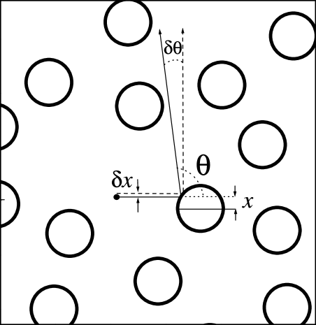
Figure 1: Schematics of a Lorentz gas showing the dispersion of two trajectories initially close to each other (with a difference $\delta x$ in the impact parameter $x$). The angle $\delta\theta$ between the two trajectories increases after each collision as described in the text.

The chaotic character of the dynamics is a consequence of the de-focusing nature of the collisions. As illustrated in Fig. 1, a particle with impact parameter $x$ will be reflected with an angle

$$\theta=\pi-2\arctan\left[\frac{x}{\sqrt{R^{2}-x^{2}}}\right].$$ (38)

If we consider a second particle with impact parameter $x+\delta x,$ its outgoing angle will be $\theta+\delta\theta,$ with

$$\delta\theta=\frac{2}{\sqrt{R^{2}-x^{2}}}\ \delta x.$$ (39)

The separation between the two particles that have traveled a distance $s$ after the collision will grow as

$$\delta d\simeq\delta x+\delta\theta s\simeq\delta x\left(1+\frac{2s}{\sqrt{R^{2}-x^{2}}}\right).$$ (40)

The next collision will further amplify the separation, due to the new impact parameters and the different incidence angles.

Within the above restrictions, the exclusion distance $R_{\mathrm{e}}$ completely determines the dynamical properties of the Lorentz gas. Among them, we are interested in the Lyapunov exponent (measuring the rate of separation of two nearby trajectories), the elastic mean free path $\ell$ (given by the typical distance between two collisions), and the transport mean free path $\ell_{\mathrm{tr}}$ (defined as the distance over which the momentum is randomized and the dynamics can be taken as effectively diffusive).

A shifted Poisson distribution

$$P(s)=\left\{\begin{array}[c]{cl}{\displaystyle{\frac{\exp\left[-s/(\ell-2(R_{\mathrm{e}}-R))\right]}{(\ell-2(R_{\mathrm{e}}-R))\exp\left[-2(R_{\mathrm{e}}-R)/(\ell-2(R_{\mathrm{e}}-R))\right]}}}&\hskip 28.45274pt\mbox{if $s>2(R_{\rm e}-R)$}\ ,\\ 0&\hskip 28.45274pt\mbox{if $s<2(R_{\rm e}-R)$}\ ,\end{array}\right.$$ (41)

is a reasonable guess for the distribution of lengths between successive collisions, which yields $\left\langle s\right\rangle=\ell=v/\tau_{\mathrm{e}}$, and is consistent with numerical simulations in the range of anti-dot concentration that we are interested in (see Fig. 2). Since velocity both $v_{0}$ and momentum $p_{0}$ are conserved within this model we will drop their subindex.

The elastic mean free path that we obtain from Fig. 2 compares favorably with a simple estimation of the mean free distance in a strip of length $L$ and width $2R$ with $2cL/\pi R$ disks,

$$\ell\simeq\frac{\pi R}{2c}\ -\ \frac{\pi R}{2}=\frac{R_{\mathrm{e}}^{2}}{0.35R}\ -\ \frac{\pi R}{2}.$$ (42)

Figure 2: Histogram of the distances between collisions with the disks, used in order to obtain numerically the mean free path $\ell$ for the Lorentz gas. The solid line represents Eq. (41) and the dash-dotted vertical line the cut-off distance $2(R_{\mathrm{e}}-R)$.

The diffusive character of the Lorentz gas can be put in evidence from the time evolution of the root mean square displacement over a collection of initial conditions. We numerically obtain $\left\langle r^{2}(t)\right\rangle=2dDt$ (with $d=2$). $\tau_{\mathrm{tr}}=\ell_{\mathrm{tr}}/v$ is the mean time required to randomize the direction and $D=v\ell_{\mathrm{tr}}/2d$ is the diffusion coefficient. The difference between $\ell$ and $\ell_{\mathrm{tr}}$ arises from the angular dependence of the scattering cross section. Taking this factor into account we obtain a ratio $\ell_{\mathrm{tr}}/\ell$ which is in good agreement with the one obtained from the independently determined $\ell$ and $\ell_{\mathrm{tr}}.$

There are known various estimations of the Lyapunov exponent of the Lorentz gas in different regimes. Considering the three-disk problem, Gaspard et al. cit-Gaspard obtained

$$\lambda=\frac{v}{2R_{\mathrm{e}}-2R}\ \ln\left[\frac{2R_{\mathrm{e}}-R+\left(4R_{\mathrm{e}}^{2}-4R_{\mathrm{e}}R\right)^{1/2}}{R}\right]\ .$$ (43)

Considering a periodic Lorentz gas (repeated Sinai billiard) Laughlin proposed the form cit-Laughlin

$$\lambda=\frac{v}{\ell}\ \ln\left[1+\frac{\beta\ell}{R}\right]\ ,$$ (44)

where $\beta$ is a geometrical factor of order $1.$ In the diluted limit ($c\ll 1$), van Beijeren and Dorfman cit-BeijerenDorfman showed that

$$\lambda=2\ \frac{N}{L^{2}}\ Rv\left(1-\ln 2-0.577-\ln\left[\frac{NR^{2}}{L^{2}}\right]\right).$$ (45)

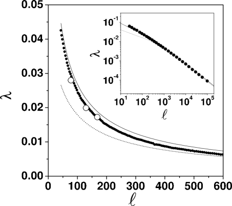
Figure 3: Lyapunov exponent $\lambda$ of the Lorentz gas as a function of the mean free path $\ell$. The black dots represent our numerical values and the solid line the analytical estimate of Eq. (48). The dashed line indicates Laughlin’s approximation (Eq. (44) and the open dots are the quantum values obtained from the decay of the LE (Fig. 6 in the sequel). Inset: the same plot in log-log scale highlighting the agreement between the different approximations in the region of very small concentrations (large $\ell$).

Numerically, the procedure of Benettin et al. cit-Lyapunov is usually followed in order to obtain Lyapunov exponents. Two nearby trajectories are followed, and their separation is scaled down to the initial value $\delta x_{0}$ after a characteristic time $t$ (that we take it to be larger than the collision time). We can then limit the numerical errors, and avoid entering the diffusive regime where two initially close trajectories follow completely independent paths. The Lyapunov exponent results from the average over the expanding rates in the different intervals,

$$\lambda=\lim_{n\rightarrow\infty}\frac{v}{n}\ \sum_{j=1}^{n}\frac{1}{s_{j}}\ \ln\left[\frac{\delta x_{j}}{\delta x_{0}}\right]\ ,$$ (46)

where $s_{j}$ is the length of the $j$-th interval, and $\delta x_{j}$ the separation just before the normalization. Technically, we should work with distances in phase-space, rather than in configuration space, but the local instability makes this precision unnecessary.

Benettin’s algorithm can also be used for a semi-analytical calculation of the Lyapunov exponent. Taking the length distribution of Eq. (41) to obtain the average separation after a collision from Eq. (40), and identifying the average over pieces of the trajectory with a geometrical average over impact parameters, we can write

$$\lambda=\frac{v}{R\ell}\ \int_{0}^{R}dx\ \ln{\left[1+\frac{2\ell}{\sqrt{R^{2}-x^{2}}}\right]}\ .$$ (47)

Performing the integration yields

$$\frac{\lambda}{v}=\frac{1}{\ell}\ \ln{\left[\frac{\ell}{R}\right]}+\frac{\pi}{R}+\sqrt{\frac{4}{R^{2}}-\frac{1}{\ell^{2}}}\ \left(\arcsin{\left[\frac{R}{2\ell}\right]}-\frac{\pi}{2}\right)\ .$$ (48)

As shown in Fig. 3, the above expression reproduces remarkably well the numerical calculations of the Lyapunov exponent. It agrees also with the result of van Beijeren and Dorfman in the dilute limit, and gives good agreement with Laughlin’s estimation.

III.2 Perturbation Hamiltonian

The quantum and classical fidelity measure the sensitivity of a given system to a perturbation of its Hamiltonian. In Ref. cit-Jalabert-Past, a quenched disorder environment was taken as the perturbation and the relaxation rate was found to depend only on the system Hamiltonian; the details of the perturbation are not important beyond some critical strength. Subsequent works have tried this perturbation cit-SmoothBilliard and others cit-PhysicaA ^-cit-Mirlin confirming the universality of the result of Ref. cit-Jalabert-Past, . It is also useful to verify such an universality by considering completely different perturbations on a given system. The Lorentz gas is an ideal case, since it can be perturbed by a quenched disorder or by the distortion of the mass tensor, introduced in Ref. cit-Lorentzgas, and briefly discussed in the sequel.

The isotropic mass tensor of $\mathcal{H}_{0},$ of diagonal components $m_{0},$ can be distorted by introducing an anisotropy such that $m_{xx}=m_{0}(1+\alpha)$ and $m_{yy}=m_{0}/(1+\alpha).$ This perturbation is inspired by the effect of a slight rotation of the sample in the problem of dipolar spin dynamics cit-QZeno , which modifies the mass of the spin wave excitations. The kinetic part of the Hamiltonian is now affected by the perturbation, that writes as

$$\Sigma(\alpha)=\alpha\ \frac{p_{y}^{2}}{2m_{0}}-\frac{\alpha}{1+\alpha}\ \frac{p_{x}^{2}}{2m_{0}}.$$ (49)

In our analytical work we will stay within the leading order perturbation in $\alpha$. That is,

$$\Sigma(\alpha)=\frac{\alpha}{2m_{0}}\ \left(p_{y}^{2}-p_{x}^{2}\right).$$ (50)

Making the particle “heavier” in the $x$ direction (i.e. we consider a positive $\alpha)$ modifies the equations of motion without changing the potential part of the Hamiltonian. It is important to notice that, unlike the case of quenched disorder, the perturbation (49) is non-random, and will not be able to provide any averaging procedure by itself, but through the underlying chaotic dynamics.

Numerical simulations of the evolution of two trajectories with the same initial conditions, the first one governed by $\mathcal{H}_{0}$ and the second one by $\mathcal{H}_{0}+\Sigma,$ show that the distance in phase space grows exponentially with the same Lyapunov exponent that amplifies initial distances. The classical dynamics is then equally sensitive to changes in the Hamiltonian as to changes in the initial conditions cit-Shack-Caves .

For a hard wall model, like the one we are considering, the perturbation (49) is equivalent to having non-specular reflections. One can resort to the minimum-action principle (see appendix A) to obtain a generalized reflection law:

$$v_{x}^{\prime} =\frac{v_{x}(m_{x}n_{y}^{2}-m_{y}n_{x}^{2})-2v_{y}m_{y}n_{x}n_{y}}{m_{x}n_{y}^{2}+m_{y}n_{x}^{2}}\ ,$$ (51a)

$$\displaystyle v_{y}^{\prime} =\frac{v_{y}(m_{y}n_{x}^{2}-m_{x}n_{y}^{2})-2v_{x}m_{x}n_{x}n_{y}}{m_{x}n_{y}^{2}+m_{y}n_{x}^{2}}\ .$$ (51b)

where $v_{x}^{\prime}$ and $v_{y}^{\prime}$ are the two components of the velocity after a collision against a surface defined by its normal unitary vector $(n_{x},n_{y}).$ Eqs. (51) allow to show that the distortion of the mass tensor is equivalent to an area conserving deformation of the boundaries as $x\rightarrow x(1+\xi)$, $y\rightarrow y/(1+\xi),$ as used in other works on the LEcit-Bunimovich , where $\xi=\sqrt{1+\alpha}-1$ is the stretching parameter. An illustrative example of the equivalence of the perturbations is shown for a stretched stadium billiard in Fig. 4. In panel $a$, a typical trajectory is shown; while in panels $b$ and $c$ we see the trajectories resulting of a perturbation of the mass tensor or the stretch of the boundaries respectively.

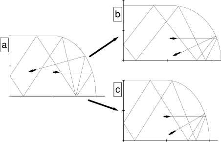
Figure 4: A single typical trajectory on the (hard wall) Bunimovich stadium, the arrows indicate the initial and final positions of the particle. (a) Normal stadium (b) Stretched stadium. (c) Normal stadium and particle with a perturbed mass, Eqs. (49). The strengths of the stretching and the mass distortion are such that the initial condition renders the same trajectory in both cases, illustrating the corresponding map (see text).

III.3 Semiclassical Loschmidt echo

We calculate in this chapter the Loschmidt echo for the system whose classical counterpart was previously discussed; $\mathcal{H}_{0}$ describes a Lorentz gas and $\Sigma$ is given by Eq. (49). We adapt to the present perturbation the semiclassical approach of Sect. II and Ref. cit-Jalabert-Past, . As before, we take as initial state a Gaussian wave-packet of width $\sigma$ (Eq. (5)).

The semiclassical approach to the LE under a weak perturbation $\Sigma$ is given by Eq. (16), with the extra phase

$$\Delta S_{s}=\int_{0}^{t}\mathrm{d}\overline{t}\ \Sigma_{s}(\mathbf{q(}\overline{t}),\mathbf{\dot{q}(}\overline{t})).$$ (52)

The sign difference with Eq. (15) is because the perturbation is now in the kinetic part of the Hamiltonian. On the other hand, as explained before, this sign turns out to be irrelevant.

With the perturbation of Eq. (50) we have to integrate a piecewise constant function (in between collisions with the scatterers), obtaining

$$\Delta S_{s}=\frac{\alpha m_{0}}{2}\ \sum_{i=1}^{N_{s}}\tau_{i}\left(2v_{y_{i}}^{2}-v^{2}\right).$$ (53)

We have used $v_{x}^{2}+v_{y}^{2}=v^{2},$ and have defined $\tau_{i}$ as the free flight time finishing with the $i$-th collision, $v_{y_{i}}$ is the $y$ component of the velocity in such an interval, and $N_{s}$ as the number of collisions that suffers the trajectory $s$ during the time $t$.

As we saw in chapter III.1, the free flight times $\tau_{i}$ (or the inter-collision length $v\tau_{i})$ have a shifted Poisson distribution (Eq. (41) and Fig. 2). This observation will turn out to be important in the analytical calculations that follow since the sum of Eq. (53) for a long trajectory can be taken as composed of uncorrelated random variables following the above mentioned distribution. It is important to remark that, unlike the case of Sec. II, the randomness is not associated with the perturbation (which is fixed), but with the diffusive dynamics generated by $\mathcal{H}_{0}$.

III.4 Non-diagonal contribution

As in the case of Sec. II, the non-diagonal contribution is given by the second moment

$$\left\langle\Delta S_{s}^{2}\right\rangle=\frac{\alpha^{2}m_{0}^{2}}{4}\ \left\langle\sum_{i,j=1}^{N_{s}}\tau_{i}\tau_{j}\left(2v_{y_{i}}^{2}-v^{2}\right)\left(2v_{y_{j}}^{2}-v^{2}\right)\right\rangle\ .$$ (54)

Separating in diagonal ($i=j$) and non-diagonal ($i\neq j$) contributions (in pieces of trajectory) we have

$$\left\langle\Delta S_{s}^{2}\right\rangle=\frac{\alpha^{2}m_{0}^{2}N_{s}}{4}\left[\left\langle\tau_{i}^{2}\right\rangle\left(4\left\langle v_{y_{i}}^{4}\right\rangle-4v^{2}\left\langle v_{y_{i}}^{2}\right\rangle+v^{4}\right)+\left(N_{s}-1\right)\left\langle\tau_{i}\right\rangle^{2}\left(4\left\langle v_{y_{i}}^{2}\right\rangle^{2}-4v^{2}\left\langle v_{y_{i}}^{2}\right\rangle+v^{4}\right)\right].$$ (55)

We have assumed that different pieces of the trajectory ($i\neq j$) are uncorrelated, and that within a given piece $i,$ $\tau_{i}$ and $v_{y_{i}}$ are also uncorrelated. According to the distribution of time-of-flights (41) we have

$$\left\langle\tau\right\rangle =\tau_{\mathrm{e}}\ ,$$ (56a)

$$\displaystyle\left\langle\tau^{2}\right\rangle =2\tau_{\mathrm{e}}^{2}\ .$$ (56b)

Assuming that the velocity distribution is isotropic ($P(\theta)=1/2\pi$, where $\theta$ is the angle of the velocity with respect to a fixed axis) is in good agreement with our numerical simulations, and results in

$$\left\langle v_{y}^{2}\right\rangle =v^{2}\left\langle\sin^{2}\theta\right\rangle=\frac{v^{2}}{2}\ ,$$ (57a)

$$\displaystyle\left\langle v_{y}^{4}\right\rangle =v^{4}\left\langle\sin^{4}\theta\right\rangle=\frac{3v^{4}}{8}\ .$$ (57b)

We thus obtain that $4\left\langle v_{y_{i}}^{2}\right\rangle^{2}-4v^{2}\left\langle v_{y_{i}}^{2}\right\rangle+v^{4}=0,$ implying a cancellation of the cross terms of $\left\langle\Delta S_{s}^{2}\right\rangle$, consistently with the lack of correlations between different pieces that we have assumed. We therefore have

$$\left\langle\Delta S_{s}^{2}\right\rangle=\frac{\alpha^{2}m_{0}^{2}N_{s}\tau_{\mathrm{e}}^{2}v^{4}}{4}\ .$$ (58)

For a given $t,$ $N_{s}$ is also a random variable, but for $t\gg\tau_{\mathrm{e}}$ we can approximate it by its mean value $t/\tau_{\mathrm{e}}$ and write

$$\left\langle\Delta S_{s}^{2}\right\rangle=\frac{\alpha^{2}m_{0}^{2}v^{4}\tau_{\mathrm{e}}t}{4}\ .$$ (59)

We therefore have for the average echo amplitude

$$\left\langle m(t)\right\rangle\simeq\exp{\left[-\frac{\alpha^{2}m_{0}^{2}v^{4}\tau_{\mathrm{e}}t}{8\hbar^{2}}\right]}\left(\frac{\sigma^{2}}{\pi\hbar^{2}}\right)^{d/2}\int d\mathbf{r}\sum_{s}C_{s}\exp{\left[-\frac{\sigma^{2}}{\hbar^{2}}\left({\overline{\mathbf{p}}}_{s}-\mathbf{p}_{0}\right)^{2}\right]}=\exp{\left[-\frac{vt}{2\tilde{\ell}}\right]}\ ,$$ (60)

where we have again used $C_{s}$ as a Jacobian of the transformation from $\mathbf{r}$ to ${\overline{\mathbf{p}}}_{s}$ and we have defined an effective mean free path of the perturbation by

$$\frac{1}{\tilde{\ell}}=\frac{m_{0}^{2}v^{2}\ell}{4\hbar^{2}}\ \alpha^{2}\ .$$ (61)

The effective mean free path $\tilde{\ell}=v~{}\tilde{\tau}$ should be distinguished from $\ell=v\tau_{\mathrm{e}}$ since the former is associated to the dynamics of $\Sigma$ and $\mathcal{H}_{0}$, while the latter is only fixed by $\mathcal{H}_{0}$. Obviously, our results are only applicable in the case of a weak perturbation verifying $\tilde{\ell}\gg\ell$. From Eq. (60) we obtain the non-diagonal component of the LE as

$$M^{\mathrm{nd}}(t)=\left|\left\langle m(t)\right\rangle\right|^{2}=\exp\left[-\frac{vt}{\tilde{\ell}}\right]\ .$$ (62)

In the next chapters we study the conditions under which the correlations not contained in the FGR approximation dominate the LE, while in Sec. IV we will test the above results against numerical simulations.

III.5 Diagonal contribution

As in Sec. II, we have to discuss separately the contribution to the LE (Eq. (16)) originated by pairs of trajectories $s$ and $s^{\prime}$ that remain close to each other. In that case the terms $\Delta S_{s}$ and $\Delta S_{s^{\prime}}$ are not uncorrelated. The corresponding diagonal contribution to the LE is given by Eq. (28), and then we have to calculate the extra actions for $s\simeq s^{\prime}$. As in Fig. 1, we represent by $\theta$ ($\theta+\delta$) the angle of the trajectory $s$ ($s^{\prime}$) with a fixed direction (i.e. that of the $x$-axis). We can then write the perturbation (Eq. (49)) for each trajectory as

$$\Sigma_{s} =\frac{\alpha}{2m_{0}}\ p^{2}\ (2\sin^{2}\theta-1)\ ,$$ (63a)

$$\displaystyle\Sigma_{s^{\prime}} =\frac{\alpha}{2m_{0}}\ p^{2}\ (2\sin^{2}\theta-2\delta\sin 2\theta-1)+\mathcal{O}(\delta^{2})\ .$$ (63b)

Assuming that the time-of-flight $\tau_{i}$ is the same for $s$ and $s^{\prime}$ we have

$$\Delta S_{s}-\Delta S_{s^{\prime}}=\frac{\alpha p^{2}}{m_{0}}\int_{0}^{t}d\overline{t}\ \delta(\overline{t})\ \sin{\left[2\theta(\overline{t})\right]}\ .$$ (64)

The angles $\delta$ alternate in sign, but the exponential divergence between nearby trajectories allows to approximate the angle difference after $n$ collisions as $\left|\delta_{n}\right|=\left|\delta_{1}\right|e^{\lambda n\tau_{\mathrm{e}}}$. A detailed analysis of the classical dynamics shows that the distance between the two trajectories grows with the number of collisions as $d_{1}=\left|\delta_{1}\right|v\tau_{1},$ $d_{2}=d_{1}+\left|\delta_{2}\right|v\tau_{2},$ and therefore

$$d_{N_{s}}\simeq v\sum_{j=1}^{N_{s}}\left|\delta_{j}\right|\tau_{j}\simeq v\tau_{\mathrm{e}}\left|\delta_{1}\right|\ \sum_{j=1}^{N_{s}}e^{(j-1)\lambda\tau_{\mathrm{e}}}=\ell\ \left|\delta_{1}\right|\ \frac{e^{N_{s}\lambda\tau_{\mathrm{e}}}-1}{e^{\lambda\tau_{\mathrm{e}}}-1}\ .$$ (65)

By eliminating $\left|\delta_{1}\right|$ we can express an intermediate angle $\delta(\overline{t})$ as a function of the final separation $\left|\mathbf{r}-\mathbf{r}^{\prime}\right|=d_{N_{s}}$,

$$\delta(\overline{t})\simeq\frac{\left|\mathbf{r}-\mathbf{r}^{\prime}\right|}{\ell}\ \frac{e^{\lambda\tau_{\mathrm{e}}}-1}{e^{\lambda t}-1}e^{\lambda\overline{t}}\ ,$$ (66)

where again we have used that $t=N_{s}\tau_{\mathrm{e}}$ is valid on average. Assuming that the action difference is a Gaussian random variable, in the evaluation of Eq. (28) we only need its second moment

$$\left\langle\left(\Delta S_{s}-\Delta S_{s^{\prime}}\right)^{2}\right\rangle\simeq\alpha^{2}m_{0}^{2}v^{4}\ \frac{\left|\mathbf{r}-\mathbf{r}^{\prime}\right|^{2}}{\ell^{2}}\ \left(\frac{e^{\lambda\tau_{\mathrm{e}}}-1}{e^{\lambda t}-1}\right)^{2}\ \left\langle\int_{0}^{t}\mathrm{d}\overline{t}\int_{0}^{t}d\overline{t}^{\prime}\ e^{\lambda\overline{t}+\lambda\overline{t}^{\prime}}\ \sin{\left[2\theta(\overline{t})\right]}\ \sin{\left[2\theta(\overline{t}^{\prime})\right]}\right\rangle\ .$$ (67)

As before, we assume that the different pieces are uncorrelated and the angles $\theta_{i}$ uniformly distributed. Therefore $\left\langle\sin\left[2\theta_{i}\right]\sin\left[2\theta_{j}\right]\right\rangle=\delta_{ij}/2$ and

$$\left\langle\left(\Delta S_{s}-\Delta S_{s^{\prime}}\right)^{2}\right\rangle \simeq\frac{\alpha^{2}}{2}\left(\frac{m_{0}v^{2}}{\ell}\right)^{2}\left|\mathbf{r}-\mathbf{r}^{\prime}\right|^{2}\left(\frac{e^{\lambda\tau_{\mathrm{e}}}-1}{e^{\lambda t}-1}\right)^{2}\sum_{i=1}^{N_{s}}\left\langle\int_{t_{i-1}}^{t_{i}}\mathrm{d}\overline{t}\ e^{\lambda\overline{t}}\right\rangle^{2}$$ (68)

$$=\frac{\alpha^{2}}{2}\left(\frac{m_{0}v^{2}}{\lambda\ell}\right)^{2}\left|\mathbf{r}-\mathbf{r}^{\prime}\right|^{2}\frac{\left(e^{\lambda\tau_{\mathrm{e}}}-1\right)^{4}}{\left(e^{\lambda t}-1\right)^{2}}\frac{e^{2\lambda N_{s}\tau_{\mathrm{e}}}-1}{e^{2\lambda\tau_{\mathrm{e}}}-1}=A\ \left|\mathbf{r}-\mathbf{r}^{\prime}\right|^{2}\ ,$$ (69)

where we have taken the limit $\lambda t\gg 1$, and defined

$$A=\frac{\alpha^{2}}{2}\left(\frac{m_{0}v^{2}}{\lambda\ell}\right)^{2}\frac{\left(e^{\lambda\tau_{\mathrm{e}}}-1\right)^{3}}{e^{\lambda\tau_{\mathrm{e}}}+1}\ .$$ (70)

Our result (69) is analogous to Eq. (33) obtained in the case of a perturbation by a quenched disorder. Obviously, the factor $A$ is different in both cases, but we use the same notation to stress the similar role as just a prefactor of $M^{d}$. Performing again a Gaussian integral of $M^{\mathrm{d}}$ over $\mathbf{r}-\mathbf{r}^{\prime}$ we obtain

$$M^{\mathrm{d}}(t)=\left(\frac{\sigma^{2}}{\pi\hbar^{2}}\right)^{d}\int\mathrm{d}\mathbf{r}\sum_{s}\ C_{s}^{2}\left(\frac{2\pi\hbar^{2}}{A}\right)^{d/2}\exp{\left[-\frac{2\sigma^{2}}{\hbar^{2}}\left({\overline{\mathbf{p}}}_{s}-\mathbf{p}_{0}\right)^{2}\right]}\ .$$ (71)

Under the same assumptions than in Sec. II.4, we are lead to a result equivalent to that of Eq. (35),

$$M^{\mathrm{d}}(t)\simeq\overline{A}e^{-\lambda t},$$ (72)

with $\overline{A}=[\sigma m_{0}/(A^{1/2}t)]^{d}$. Therefore, for long times the diagonal part of the Loschmidt echo decays with a rate given by the classical Lyapunov exponent of the system,

$$\lim_{t\rightarrow\infty}\left(-\frac{1}{t}\ \ln\left[M^{\mathrm{d}}(t)\right]\right)=\lambda.$$ (73)

Of course this limit actually means $t\gg 1/\lambda$ but still lower than the time at which either localization or finite size effect appears. In the next chapter we will study the competition between the diagonal and non-diagonal contributions.

III.6 Diagonal vs. non-diagonal contributions

As we have previously shown, the Loschmidt echo is made out of non-diagonal and diagonal components, and within the time scales above specified, it can be written as

$$M(t)=\exp\left[-\frac{vt}{\tilde{\ell}}\right]+\overline{A}\exp\left[-\lambda t\right]\ .$$ (74)

Such a result holds for the perturbation $\Sigma$ that we have discussed in this section (Eq. (49)), as well as for the quenched disorder of Sec. II (Eq. (18). The only difference lays in the form of the “elastic mean free path” $\tilde{\ell}$ and the prefactor $\overline{A}$, both of which are perturbation dependent. The decay of the LE will be controlled by the slowest of the two rates. A weak perturbation implies $\tilde{\ell}>v/\lambda$ and a dominance of the non-diagonal term, while for sufficiently strong perturbations verifying $\tilde{\ell}<v/\lambda$ (but weak enough in order not to modify appreciably the classical trajectories), the diagonal term (governed by the Lyapunov exponent) sets the decay of the LE. In Ref. cit-Jacquod01, the regime of dominance of the non-diagonal and diagonal component has been respectively interpreted and referred to as a Fermi Golden Rule Lyapunov regimes and we will use both terminologies in the discussions that follow.

The Lyapunov regime is remarkable in the sense that its decay rate is an intrinsic property of the system and does not depend on the perturbation that gives rise to the decay. This behavior, predicted in Ref. cit-Jalabert-Past, has been observed in numerical simulations done on a number of systems cit-PhysicaA ^-cit-Mirlin .

From the previous discussion it is clear that the Lyapunov regime can only be observed beyond a critical value of the perturbation. The condition stated above for the strength of the perturbation, along with Eq. (61), yields for the model discussed in this section a critical value of the perturbation parameter $\alpha$ beyond which the Lyapunov regime is obtained,

$$\alpha_{\mathrm{c}}=\frac{2\hbar}{m_{0}}\sqrt{\frac{\lambda}{v^{3}\ell}}.$$ (75)

We will discuss in Sec. IV the physical consequences of the above critical value and its dependence on various physical parameters.

We finish this chapter with the discussion of the perturbation dependent (non-diagonal) regime. In this Fermi Golden Rule regime the LE is equal to the return probability $P(t)=\left|\left\langle\psi_{0}\right|\exp\left[-\mathrm{i}\left(\mathcal{H}_{0}+\Sigma\right)t/\hbar\right]\left|\psi_{0}\right\rangle\right|^{2}$, whose decay rate does not show saturation at the Lyapunov exponent but rather follows Eq. (61) for the whole range of parameterscit-WisniackiCohen . The full connection between the exponent of Eq. (61) and the one we would get from a complete FGR approach, was clarified using a random matrix treatment cit-SmoothBilliard . In fact, a rough estimation of the Fermi golden rule is obtained considering a particle moving along the principal axis $\overleftrightarrow{m}$ of a square box of sides $L_{x}=L_{y}=\ell$. The available density of states $\frac{1}{\Delta}$, corresponds to a 1-d tube of length $\ell.$ Hence

$$\frac{1}{\tilde{\tau}} =\frac{2\pi}{\hbar}\left|\Sigma\right|^{2}\frac{1}{\Delta}$$

$$\simeq\frac{2\pi}{\hbar}\left|\alpha\frac{p^{2}}{2m_{0}}\right|^{2}\times\frac{\ell m_{0}}{\pi\hbar p}$$

$$=m^{2}\frac{v^{3}}{4\hbar^{2}}\ell\alpha^{2},$$

in agreement with the semiclassical calculation of Eq. (61). Of course, this estimation does not make justice to the chaotic nature of $\mathcal{H}_{0}$. This breaks the selection rules of our simple perturbation and enables a random matrix approximation for $\Sigma$, that mixes eigenstates of $\mathcal{H}_{0}$ which follow a Wigner-Dyson statistics. Hence the perturbation breakdown of the FGR regime can not be calculated from the parameters introduced above.

The LE has also been studied in systems where the perturbation structure prevents the application of the Fermi Golden Rule. The result is that in general the decay rate of the LE before the Lyapunov regime is given by the width of the local density of states of the perturbation, which for particular systems coincides with the exponent given by the FGRcit-Bunimovich .

IV Universality of the Lyapunov regime

IV.1 Correspondence between semiclassical and numerical calculations

The semiclassical results obtained in the previous sections are valid in the small wavelength limit, and relay on various uncontrolled approximations. It is then important to perform numerical calculations for our model system in order to compare against the semiclassical predictions, and to explore parameter regimes inaccessible to the theory. In this section we use the same numerical method of Ref. cit-Lorentzgas, for the Lorentz gas (described in detail in appendix B), and extend the results in order to sustain the discussion on the universality of the Lyapunov regime. We will first focus on the behavior of the ensemble averaged Loschmidt echo, followed by a thorough discussion of the averaging procedure and the individual behavior.

We typically worked with disks of radius $R=20a$ , and with a Fermi wavelength $\lambda_{F}=2\pi/k_{F}=16/3a$. Here,  $a$ is the irrelevant lattice unit of our tight-binding model, which is decreased until the results only depend on the relation between physical parameters. The smallest system-size allowing to observe the exponential decay of $M(t)$ over a large interval was found to be $L=200a$ which means the consideration of a Hilbert space with 4$\times$10⁴ states. We calculated $M(t)$ for different strengths of the perturbation $\alpha$ and concentration of disks $c$. In Fig. 5 we show our results for $c=0.157$, $0.195$ and $0.289$ (panels $a$ to $c$ respectively), and different values of $\alpha$.

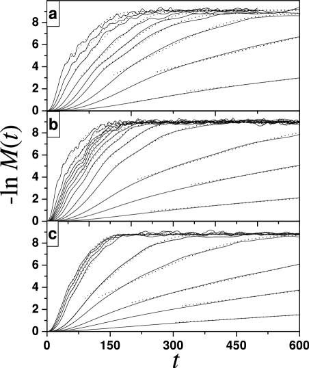
Figure 5: Time decay of the Loschmidt echo $M(t)$ for different values of the perturbation strength ($\alpha$) and concentration of impurities ($c$). (a) $c=0.157$ and $\alpha=$0.004, 0.007, 0.01, 0.015, 0.02, 0.03, 0.05, 0.07, 0.1 (from top to bottom); (b) $c=0.195$ and $\alpha=$0.004, 0.007, 0.01, 0.015, 0.02, 0.03, 0.04, 0.05, 0.06, 0.07, 0.08, 0.1, 0.15; (c) $c=0.289$ and $\alpha=$0.004, 0.007, 0.01, 0.015, 0.02, 0.03, 0.04, 0.05, 0.06, 0.07. The time is measured in units of $\hbar/V$, where $V$ is the hopping term of the tight-binding model (see appendix B). The doted lines represent the best fits to the decay, as described in the text.

The time evolution of the LE presents various regimes. Firstly, for very short times, $M(t)$ exhibits a Gaussian decay, $M(t)=\exp\left[-b\alpha^{2}t^{2}\right]$, where $b$ is a parameter that depends on the initial state, the dynamics of $\mathcal{H}_{0}$ and the form of the perturbation $\Sigma$. This initial decay corresponds to the overlap of the perturbed and unperturbed wave-packets whose centers separate linearly with time by the sole effect of the perturbation. This regime ends approximately at the typical time of the first collision.

Secondly, for intermediate times we find the region of interest for the semiclassical theory. In this time scale the LE decays exponentially with a characteristic time $\tau_{\phi}$. We reserve the symbol $\tau_{\phi}$ for the decay rate, in view of its interpretation in terms of quantum decoherence (as we discuss in Sec. V). For small perturbations, $\tau_{\phi}$ depends on $\alpha$. We observe that for all concentrations there is a critical value $\alpha_{\mathrm{c}}$ beyond which $\tau_{\phi}$ is independent of the perturbation. Clearly, the initial perturbation-dependent Gaussian decay prevents the curves to be superimposed.

Finally, for very large times the LE saturates at a value $M_{\infty}$ that depends on the system size $L$. This regime is discussed in detail in the next chapters. However, let us observe that in the crossover between the exponential decay and the long time saturation there is a power-law decay with a perturbation independent exponent. This is a manifestation of the underlying diffusive dynamics that leads to the isotropic state. Therefore, it could be related to the Ruelle-Perricot resonances of the classical Perron-Frobenius evolution operator used to calculate a classical version of the LE cit-CasatiClassic .

In order to compare our numerical results of $M(t)$ with the semiclassical predictions, we extract $\tau_{\phi}$ by fitting $\ln M(t)$ to $\ln\left[A\exp(-t/\tau_{\phi})+M_{\infty}\right].$ The dashed lines in Fig. 5 correspond to the best fits obtained with this procedure. The values of $\tau_{\phi}$ for the different concentrations are shown as a function of the perturbation strength in Fig. 6. In agreement with our analytical results of the previous section, we see that $1/\tau_{\phi}$ grows quadratically with the perturbation strength up to a critical value $\alpha_{\mathrm{c}}$, beyond which a plateau appears at the corresponding Lyapunov exponent. The dashed lines are the best fit to a quadratic behavior. The values obtained in this way agree with those predicted by the semiclassical theory (Eq. (61)) for the non-diagonal (FGR) term. The saturation values above $\alpha_{\mathrm{c}}$ are well described by the corresponding Lyapunov exponents (solid lines), in agreement with the semiclassical prediction (Eq. (73)). The very good quantitative agreement between the semiclassical and numerical calculations for the Lorentz gas (as well as in the case of other models cit-Jacquod01 ; cit-Bunimovich ; cit-SmoothBilliard ) strongly supports the generality of the saturation of $\tau_{\phi}$ at a critical value of the perturbation strength.

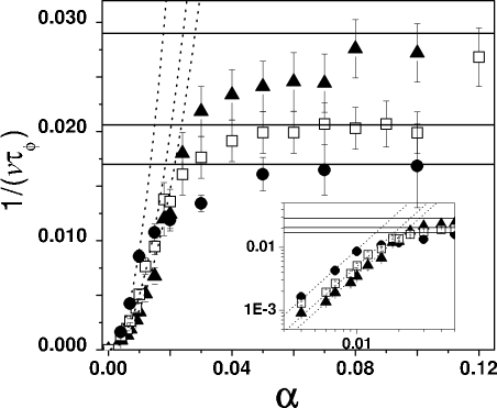
Figure 6: Extracted values of the decay rate $1/\tau_{\phi}$ of the LE as a function of the perturbation strength $\alpha$ for the three concentrations of Fig. 5. The rates are normalized to the group velocity of the initial wave-packet $\nu$ ($1/(\nu\tau_{\phi})$) is given in units of $a^{-1}$; $c=0.157$ (circles), $0.195$ (squares) and $c=0.289$ (triangles). The solid lines are the corresponding classical Lyapunov exponents and the dashed lines are fits to the quadratic behavior predicted by Eq. (61). The predicted coefficients for the three concentrations are $72a^{-1}$, $55a^{-1}$ and $33a^{-1}$, while the obtained ones are $92a^{-1}$, $50a^{-1}$ and $37a^{-1}$ respectively. In the inset, a log-log scale of the same data to show the quadratic increase of $1/\tau_{\phi}$ for small perturbations.

The FGR exponent, which depends on $\mathcal{H}_{0}$ but not much on its chaoticity cit-JacquodInt , is given by the typical squared matrix element of $\Sigma$, and the density of connected final states $1/\Delta$. Hence, different $\mathcal{H}_{0}$ change the wave-functions. That is why we observe that, for fixed perturbation strength $\alpha$, the factor $v/\tilde{\ell}$ depends on the concentration of impurities of $\mathcal{H}_{0}$ (see inset of Fig. 6, where a log-log scale has been chosen in order to magnify the small perturbation region).

Notably, the dependence of $v/\tilde{\ell}$ with $\mathcal{H}_{0}$ leads to a counter-intuitive effect (clearly observed in the inset of Fig. 6), namely that the critical value needed for the saturation of $1/\tau_{\phi}$ is smaller for less chaotic systems (smaller $\lambda$). The reason for this is that in more dilute systems $\Sigma$ is constant over larger straight pieces of trajectories (in between collisions), leading to a larger perturbation of the quantum phase and resulting in a stronger effective perturbation.

IV.2 Universality of the Lyapunov regime in the semiclassical limit

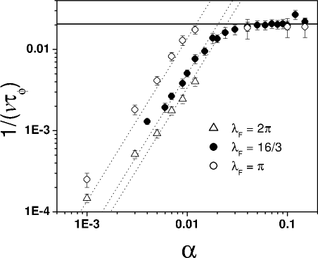
Figure 7: Decay rates $1/\tau_{\phi}$ for different wavelengths $\lambda_{F}$ of the initial wave-packet for a concentration $c=0.195$ with the same units as in Fig 6. Solid line: classical Lyapunov exponent. Dashed line: the FGR quadratic behavior. Note that for decreasing $\lambda_{F}$ the critical perturbation diminishes, implying a collapse of the Fermi Golden Rule regime.

Our semiclassical analysis yielded a critical value of the perturbation to enter in the Lyapunov regime (Eq. (75)), that vanishes in the semiclassical limit, $\alpha_{\mathrm{c}}\rightarrow 0$ for $\hbar$ (or $\lambda_{F}$) $\rightarrow 0$, implying the collapse of the Fermi Golden Rule regime. This behavior is reproduced by our numerical calculations (Fig. 7). There, we decreased $\lambda_{F}$ while keeping fixed the size $\sigma$ of the initial wave packet. A point that should not be over-sighted is that the perturbation $\Sigma$ (Eq. (49)), for a given value of the parameter $\alpha$, scales with the energy in a way that the underlying classical trajectories are always affected in the same way by the perturbation. The extracted crossover values of $\alpha_{\mathrm{c}}$ are in quantitative agreement with Eq. (75), decreasing with $\lambda_{F}$ in the interval that we were able to test.

Other choices of the perturbation $\Sigma$, such as the quenched disorder of Refs. cit-Jalabert-Past, and cit-SmoothBilliard, , can be shown to give critical values that decrease with decreasing $\hbar$ as in Eq. (75), provided that the perturbation is scaled to the proper semiclassical limit. That is, for a fixed perturbation potential, we should take the limit of $\lambda_{F}\rightarrow 0$. As a result, if we keep $\hbar$ constant and decrease $\lambda_{F}$ by increasing the particle energy, we should scale up the perturbation potential consistently (assuming that $\mathcal{H}_{0}$ generates the same dynamics at all energies).

We conclude that, in the semiclassical limit, any perturbation will be strong enough to put us in the Lyapunov regime, in consistency with the hypersensitivity expected for a classical system. This is not unexpected as in this limit the Ehrenfest time diverges and the correspondence principle should prevail.

We can draw a the critical perturbation strength separating FGR from Lyapunov regimes versus a scaling parameter determined by the particle energy (or inverse $\hbar$), as shown in Fig. 8. The shaded region corresponds to the Fermi Golden Rule regime and the clear one to the Lyapunov regime. The line that divides both phases is given by Eq. (75), and the dots correspond to numerical values of $\alpha_{\mathrm{c}}$ extracted from Figs. 6 and 7. Of course, there is another transition from FGR to perturbation appearing when $\Sigma\simeq\Delta,$ which we avoid drawing since $\alpha_{\Delta}\ll\alpha_{\mathrm{c}}$. This perturbative value also goes to zero in the semiclassical limit of $\lambda_{F}\rightarrow 0.$ Also the Lyapunov regime is bounded from above by an $\hbar$ independent critical value $\alpha_{\mathrm{p}}$ marking the classical breakdown that we discuss bellow.

The interesting conceptual feature highlighted by Fig. 8, is the importance of the order in which we take the limits of $\Sigma$ and $\lambda_{F}$ going to zero. Two distinct results are obtained for the different order in which we can take this double limit. As depicted in the figure (with arrows representing the limits), $\lim_{\lambda_{F}\rightarrow 0}\lim_{\Sigma\rightarrow 0}1/\tau_{\phi}=0$. On the other hand, taking the inverse (more physical) ordering $\lim_{\Sigma\rightarrow 0}\lim_{\lambda_{F}\rightarrow 0}1/\tau_{\phi}=\lambda$ the semiclassical result is obtained. The resulting “phase diagram” representation for the different regimes of the LE serves us to remember that most often one is working in the thermodynamic side corresponding to the Lyapunov region.

Our semiclassical theory clearly fails when the perturbation is strong enough (or the times long enough) to appreciably modify the classical trajectories. This would give an upper limit (in perturbation strength) for the results of Sec. III. A more stringent limitation comes from the finite value of $\hbar$, due to the limitations of the diagonal approximations and linear expansions of the action that we have relied on. In other systems, like the quenched disorder in a smooth stadium cit-SmoothBilliard , the upper critical value of the perturbation (for exiting the Lyapunov regime) can be related to the transport mean free path of the perturbation $\tilde{\ell}_{\mathrm{tr}}$, which is defined as the length scale over which the classical trajectories are affected by the disorderJMP .

We can obtain in our system an estimate of $\tilde{\ell}_{\mathrm{tr}}$ by considering the effect of the perturbation on a single scattering event. The difference $\delta\theta$ between the perturbed and unperturbed exit angles after the collision can be obtained using Eqs. (51), which results in

$$\delta\theta\sim 4n_{x}n_{y}\left(\frac{\mathbf{v}\cdot\mathbf{n}}{v}\right)^{2}\ \alpha\ ,$$ (76)

where $\mathbf{v}$ is the initial velocity of the particle and $\mathbf{n}$ is the normal to the surface.

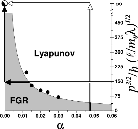
Figure 8: Regime diagram for the Loschmidt echo as a function of the perturbation and the energy (or inverse $\hbar$). The grayed area is the FGR regime, while the clear one is the Lyapunov regime. The line that divides both regimes is Eq. (75). The dots are the numerical values obtained from Figs. 6 and 7. The arrows schematize the possible ordering of the classical double limit of the perturbation and the wavelength going to zero. Notice how the lower one gives always zero while the upper (correct) one gives $\lambda$ since it remains always in the Lyapunov regime.

Assuming that the movement of the particle is not affected by chaos (non-dispersive collisions), one can do a random walk approach and estimate the mean square distance after a time $\tau_{tr}$ from the fluctuations of the angle in Eq. (76). We estimate the transport mean free time as that at which the fluctuations are of the order of $R$, and obtain

$$\tilde{\ell}_{\mathrm{tr}}\simeq\frac{4R^{2}}{3\alpha^{2}\ell}\ ,$$ (77)

assuming a uniform probability for the angle of the velocity as before. Eq. (77) is used to get the upper bound perturbation $\alpha_{\mathrm{p}}$ for the end of the Lyapunov plateau,

$$\alpha_{\mathrm{p}}=\sqrt{\frac{4\lambda R^{2}}{3\ell v}}\ .$$ (78)

We obtain $\alpha_{\mathrm{p}}\simeq 0.23,$ $0.29$ and $0.43$ respectively for increasing magnitude of the three concentrations shown in Fig. 6. It is rather difficult to reach numerically these perturbations in our system, since the initial Gaussian decay drives $M(t)$ very quickly towards its saturation value, preventing the observation of an exponential regime. Despite this difficulty, we observe in Fig. 7 that Lyapunov regime is a plateau that ends up for sufficiently strong perturbations. For the range we could explore the limiting values are in qualitative agreement with the estimation from Eq. (78).

IV.3 Ehrenfest time and thermodynamic limit

We studied in the previous chapter the behavior of the Lyapunov regime in the semiclassical limit $\hbar\rightarrow 0$; let us now turn our attention to the consequences of having a finite value of $\hbar$. In this case, one expects the propagation of a quantum wave-packet to be described by the classical equations of motion up to the Ehrenfest time $t_{E}$, after which the quantum-classical correspondence breaks down cit-BermanZavslasky . Typically, $t_{E}$ is the time when interference effects become relevant, and in a classically chaotic system it typically scales as $\ln[\hbar]$.

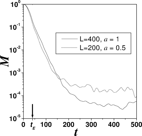
Figure 9: $M(t)$ for two systems with the same number of states $N$ but different sizes $L$, showing that the saturation time does not depend on $N$ but on the ratio $L/\sigma$. The Ehrenfest time is marked with an arrow.

In other systems where the Lyapunov regime of the LE has been observed, such as chaotic maps or kicked systems, $t_{E}$ coincides with the saturation time $t_{s}=1/\lambda$ $\ln[N]$. This is because in these systems the number of states $N$ plays the role of an effective Planck’s constant $\hbar_{\mathrm{eff}}=1/N$. Therefore, when in these systems the LE is governed by a classical quantity, the whole range of interest occurs before the Ehrenfest time. This observation lead Benenti and Casaticit-BenentiCasati to propose that the independence of the decay rate on the perturbation strength is a trivial consequence of the quantum-classical correspondence before $t_{E}$.

In the Lorentz gas, however, we can differentiate between the time scales $t_{s}$ and $t_{E}$ by appropriately controlling the parameters. The saturation time is given by

$$t_{s}\simeq\frac{2}{\lambda}\ln\frac{L}{\sigma}\ .$$ (79)

The Ehrenfest time, defined as the time it takes for a minimal wave-packet of wavelength $\lambda_{F}$ to spread over a distance of the order of $R$ cit-AleinerLarkin , is given by

$$t_{E}\simeq\frac{1}{\lambda}\ln\frac{2R}{\lambda_{F}}\ .$$ (80)

Our numerical calculations support these approximations. We show in Fig. 9 $M(t)$ for two systems with the same number of states $N$ (hence same $\hbar_{\mathrm{eff}}$), but two different sizes $L$. $N$ is controlled by the discretization step $a=L/N$. The different saturation values (and times) observed imply that for the Lorentz gas $t_{E}$ and $t_{s}$ are independent of each other. Clearly we can study the LE for times arbitrarily larger than $t_{E}$ by increasing the system size $L,$ which controls $t_{s},$ and keeping all other parameters (including $t_{E}$, marked with a dashed line in Fig. 9) fixed. We can see that the exponential decay of the LE continues for times larger than $t_{E}$, up to the saturation time.

The above results are further evidence of the universality of the Lyapunov regime, for it persists for arbitrarily large times in the thermodynamic limit of the size of the system going to infinity. This is exemplified in Fig. 10, where we show $M(t)$ for increasing sizes ($L=200a,400a$ and $800a$) for a fixed concentration ($c=0.195$) and perturbation ($\alpha=0.024$). Notice how the exponential decay regime extends, as $L$ grows, for times larger than $t_{E},$ where the correspondence principle does not prevail. The survival of a classical signature of the quantum dynamics after the Ehrenfest time is due to a more complex effect, namely the decoherence that washes out terms of quantum nature. We will discuss this process in detail in the next chapter.

Figure 10: $M(t)$ for different system sizes $L=200,400$ and $800$ showing the longer exponential regime for larger $L$. Inset: saturation value $M_{\infty}$ as a function of inverse system size. The straight line is the fit $M_{\infty}=(0.6)(\sigma/L)^{2}$.

In the inset of Fig. 10 we see the saturation value $M_{\infty}$ as a function of the inverse system size $1/L^{2}$. This dependence was expected from earlier works on the LE cit-Peres . Supposing that for long times the chaotic nature of the system will equally mix the $\tilde{N}=\left(L/\sigma\right)^{2}$ levels appreciably represented in the initial state with random phases $\phi_{j},$ we write

$$M_{\infty}=\frac{1}{\tilde{N}^{2}}\left|\sum_{j}\exp\left[\mathrm{i}(\phi_{j}-\phi_{j}^{\prime})\right]\right|^{2}=\frac{1}{\tilde{N}}\ .$$ (81)

We also show in a straight line the best fit to the data, $M_{\infty}=(0.6\pm 0.1)\left(\sigma/L\right)^{2}$ which confirms the prediction.

IV.4 Individual vs. ensemble-average behavior

In order to make analytical progress, in our semiclassical calculations and in those of Ref. cit-Jalabert-Past, , an ensemble average was introduced (over realizations of the quenched disordered perturbation or over initial conditions). This approximation raises the question of whether the exponential decay of $M(t)$ is already present in individual realizations or, on the contrary, the averaging procedure is a crucial ingredient in obtaining a relaxation rate independent of the perturbation cit-Silvestrov .

As it was discussed in Sects. II and III, for trajectories longer than the correlation length $\xi$ of the perturbation, the contributions to $\Delta S$ from segments separated by more than $\xi$ are uncorrelated. This leads us to consider that the decay observed for a single initial condition will be equivalent to that of the average. In this section we test this idea numerically.

For large enough systems presenting a large saturation time, we expect $M(t)$ to fluctuate around an exponential decay. This expectation is clearly supported by our numerical results shown in Fig. 11, where we present $M(t)$ for three different initial conditions in a system with $L=800a$ and fixed $\alpha=0.024.$ An exponential decay with the semiclassical exponent is shown for comparison (thin solid line).

Figure 11: $M(t)$ for three different single initial conditions of the wave-packet. All the curves oscillate around the straight line, which is the decay corresponding to the Lyapunov exponent.

In order to obtain the exponent of the decay with a good precision, we can calculate $M(t)$ for a single initial condition in a large enough system. Alternatively, our results show that it is correct to obtain the exponent through an ensemble average to reduce the size of the fluctuations. However, as the former method is computationally much more expensive, we resort to the latter.

This situation is analogous to the classical case where one obtains the Lyapunov exponent from a single trajectory taking the limit of the initial distance going to zero and the time going to infinity, or else resorts to more practical methods like Benettin et al algorithm that average distances over short evolutions.

Notice that in the Lorentz gas the average over initial conditions and the average over realizations of the impurities positions are equivalent. In all cases we have implemented the last choice for being computationally convenient, and we use the term initial conditions to refer also to realizations of $\mathcal{H}_{0}$.

In particular for our calculations, the average is constrained to those systems where the classical trajectory of the wave-packet collides with at least one of the scatterers. This restriction helps avoiding those configurations where a “corridor” exists, in which case $M(t)$ presents a power-law decay possibly related to the behavior found in integrable systems cit-JacquodInt .

IV.5 Effect of the average procedure

The averaging of quantities that fluctuate around an exponential decay is a delicate matter, since different procedures can lead to quite different results. In particular, for the LE it has been noted that averaging $M(t)$ over initial conditions can result in an exponential decay different than the one of a single initial condition cit-WangLi ; cit-Silvestrov . This effect can be attained, for instance, if we suppose that $M(t)$ for single conditions decays exponentially with a fluctuating exponent $\lambda+\delta\lambda$, where $\delta\lambda$ is randomly distributed with uniform probability between $-\sigma_{\lambda}$ and $\sigma_{\lambda}$. Given the exponential dependence of $M(t)$ in $\lambda$, the phase space fluctuations of the Lyapunov exponent will induce a difference between the average $\ln M(t)$ and that of $M(t)$. The former procedure is more appropriate in order to have averages of the order of the typical values. On the other hand, if the fluctuations of the exponent are small, both procedures give similar results. This is the situation we found in our model system.

For the Lorentz gas we calculated $\left\langle M(t)\right\rangle$ and $\left\langle\ln M(t)\right\rangle$ and extracted the decay rates of the exponential regime using the fit described in Sec. IV.1. Typical results are shown in Fig. 12 as a function of the perturbation. We observe that both averaging procedures give values of $\tau_{\phi}$ that are indistinguishable from each other within the statistical error.

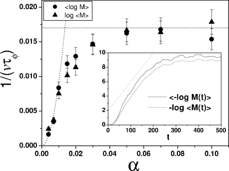
Figure 12: Values of $\tau_{\phi}$ extracted from averaging the echo $\left\langle M\right\rangle$ (triangles) and the logarithm of the echo $\left\langle\log M\right\rangle$ (circles) for $c=0.289$ and $L=200$, as a function of the perturbation strength. Both averaging procedures yield approximate the same decay rate. Inset: typical curves of $\left\langle M\right\rangle$ and $\left\langle\log M\right\rangle$ for the same set of parameters. The straight dotted line represents an exponential decay with a rate given by the semiclassical prediction.

A typical set of curves of $M(t)$ averaged following the two procedures is shown in the inset of Fig. 12. We can see that, even though for the short and long time regimes the two procedures give slightly different results, the intermediate exponential decay regime has approximately the same decay rate in both cases.

V Analysis of decoherence through the Loschmidt echo

V.1 Classical evolution of the Wigner function

As discussed in the introduction, the Loschmidt echo can be obtained from the evolution of the Wigner function with the perturbed and unperturbed Hamiltonians (Eq. (2)). Such a framework is particularly useful in the study of decoherence, as the Wigner function is a privileged tool to understand the connection between quantum and classical dynamics bookBrack ; cit-ZurekNature .

The evolution of the wave-functions in terms of the propagators (Eq. (6)) can be used to express the time-dependence of the Wigner function as

$$W(\mathbf{r},\mathbf{p};t)=\frac{1}{(2\pi\hbar)^{d}}\int\mathrm{d}\delta\mathbf{r}\int\mathrm{d}\overline{\mathbf{q}}\int\mathrm{d}{\overline{\mathbf{q}}}^{\prime}\exp{\left[\frac{\mathrm{i}}{\hbar}\ \mathbf{p}\cdot\delta\mathbf{r}\right]}\ K\left(\mathbf{r}-\frac{\delta\mathbf{r}}{2},\overline{\mathbf{q}};t\right)\ K^{\ast}\left(\mathbf{r}+\frac{\delta\mathbf{r}}{2},{\overline{\mathbf{q}}}^{\prime};t\right)\ \psi(\overline{\mathbf{q}},0)\ \psi^{\ast}({\overline{\mathbf{q}}}^{\prime},0).$$

Noting $W(\overline{\mathbf{r}},{\overline{\mathbf{p}}};0)$ the initial Wigner function, we can write

$$W(\mathbf{r},\mathbf{p};t) =\frac{1}{(2\pi\hbar)^{d}}\int\mathrm{d}\delta\mathbf{r}\int\mathrm{d}\overline{\mathbf{r}}\int\mathrm{d}\delta{\overline{\mathbf{r}}}\int\mathrm{d}{\overline{\mathbf{p}}}\ W(\overline{\mathbf{r}},{\overline{\mathbf{p}}};0)\ \exp\left[\frac{\mathrm{i}}{\hbar}(\mathbf{p}\cdot\delta\mathbf{r}-{\overline{\mathbf{p}}}\cdot\delta{\overline{\mathbf{r}}})\right]$$

$$\times\ K\left(\mathbf{r}-\frac{\delta\mathbf{r}}{2},\overline{\mathbf{r}}-\frac{\delta{\overline{\mathbf{r}}}}{2};t\right)\ K^{\ast}\left(\mathbf{r}+\frac{\delta\mathbf{r}}{2},\overline{\mathbf{r}}+\frac{\delta{\overline{\mathbf{r}}}}{2};t\right)\ .$$ (82)

The semiclassical expansion of the propagators (Eq. (8)) leads to the propagation of the Wigner function by “chords” Ozorio ; Caio ; Horacio92 , where pairs of trajectories $(s,s^{\prime})$ traveling from $(\overline{\mathbf{r}}-\delta{\overline{\mathbf{r}}}/2,\overline{\mathbf{r}}+\delta{\overline{\mathbf{r}}}/2)$ to $(\mathbf{r}-\delta\mathbf{r}/2,\mathbf{r}+\delta\mathbf{r}/2)$ have to be considered (Fig. 13). In the leading order in $\hbar$ we can approximate the above propagators by sums over trajectories going from $\overline{\mathbf{r}}$ to $\mathbf{r}$

$$K\left(\mathbf{r}-\frac{\delta\mathbf{r}}{2},\overline{\mathbf{r}}-\frac{\delta{\overline{\mathbf{r}}}}{2};t\right) =\sum_{s(\overline{\mathbf{r}},\mathbf{r},t)}\ K_{s}(\mathbf{r},\overline{\mathbf{r}};t)\ \exp\left[\frac{\mathrm{i}}{2\hbar}\left({\overline{\mathbf{p}}}_{s}\cdot\delta{\overline{\mathbf{r}}}-\mathbf{p}_{s}\cdot\delta\mathbf{r}\right)\right]\ ,$$ (83a)

$$\displaystyle K\left(\mathbf{r}+\frac{\delta\mathbf{r}}{2},\overline{\mathbf{r}}+\frac{\delta{\overline{\mathbf{r}}}}{2};t\right) =\sum_{s^{\prime}(\overline{\mathbf{r}},\mathbf{r},t)}\ K_{s^{\prime}}(\mathbf{r},\overline{\mathbf{r}};t)\ \exp\left[\frac{\mathrm{i}}{2\hbar}\left(-{\overline{\mathbf{p}}}_{s^{\prime}}\cdot\delta{\overline{\mathbf{r}}}+\mathbf{p}_{s^{\prime}}\cdot\delta\mathbf{r}\right)\right]\ ,$$ (83b)

where ${\overline{\mathbf{p}}}_{s}$ ($\mathbf{p}_{s}$) and ${\overline{\mathbf{p}}}_{s^{\prime}}$ ($\mathbf{p}_{s^{\prime}}$) are the initial (final) momenta of the trajectories $s$ and $s^{\prime}$, respectively. The semiclassical evolution of the Wigner function is given by

$$W(\mathbf{r},\mathbf{p};t)=(2\pi\hbar)^{d}\int\mathrm{d}\overline{\mathbf{r}}\int\mathrm{d}{\overline{\mathbf{p}}}\ W(\overline{\mathbf{r}},{\overline{\mathbf{p}}};0)\ \sum_{s,s^{\prime}}\ \delta\left({\overline{\mathbf{p}}}-\frac{{\overline{\mathbf{p}}}_{s}+{\overline{\mathbf{p}}}_{s^{\prime}}}{2}\right)\ \delta\left(\mathbf{p}-\frac{\mathbf{p}_{s}+\mathbf{p}_{s^{\prime}}}{2}\right)K_{s}\left(\mathbf{r},\overline{\mathbf{r}};t\right)\ K_{s^{\prime}}^{\ast}\left(\mathbf{r},\overline{\mathbf{r}};t\right)\ .$$

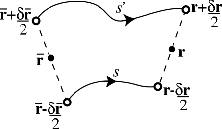
Figure 13: Schematics of the classical trajectories involved in the semiclassical approximation to the propagation of a Wigner function.

The dominant contribution arises from the diagonal term $s=s^{\prime}$

$$W_{\mathrm{c}}(\mathbf{r},\mathbf{p},t)=\int\mathrm{d}\overline{\mathbf{r}}\sum_{s(\overline{\mathbf{r}},\mathbf{r},t)}\ C_{s}\ \delta\left(\mathbf{p}-\mathbf{p}_{s}\right)\ W(\overline{\mathbf{r}},{\overline{\mathbf{p}}}_{s};0)\ .$$ (84)

Using the fact that $C_{s}$ is the Jacobian of the transformation from $\overline{\mathbf{r}}$ to $\mathbf{p}_{s}$, we have

$$W_{\mathrm{c}}(\mathbf{r},\mathbf{p};t)=\int\mathrm{d}\mathbf{p}_{s}\ \delta\left(\mathbf{p}-\mathbf{p}_{s}\right)\ W(\overline{\mathbf{r}},{\overline{\mathbf{p}}}_{s};0)\ ,$$ (85)

where the trajectories considered now are those that arrive to $\mathbf{r}$ with momentum $\mathbf{p}$. We note $(\overline{\mathbf{r}},{\overline{\mathbf{p}}})$ the pre-image of $(\mathbf{r},\mathbf{p})$ by the equations of motion acting on a time $t$. That is, $(\mathbf{r},\mathbf{p})=X_{t}(\overline{\mathbf{r}},{\overline{\mathbf{p}}})$. The momentum integral is trivial, and we obtain the obvious result

$$W_{\mathrm{c}}(\mathbf{r},\mathbf{p};t)=W(\overline{\mathbf{r}},{\overline{\mathbf{p}}};0)\ ,$$ (86)

with $(\overline{\mathbf{r}},{\overline{\mathbf{p}}})=X_{t}^{-1}(\mathbf{r},\mathbf{p})$. Since $X_{t}$ conserves the volume in phase-space, at the classical level the Wigner function evolves by simply following the classical flow.

V.2 Fine structure of the Wigner function and non-classical contributions to the Loschmidt echo

As indicated in Eq. (2), the Loschmidt echo is given by the phase-space trace of two Wigner functions associated with slightly different Hamiltonians ($\mathcal{H}_{0}$ and $\mathcal{H}_{0}+\Sigma$). In order to facilitate the discussion, we introduce the density (or partial trace) $f_{\Sigma}$ writing the LE as

$$M(t)=\int\mathrm{d}\mathbf{r}\ f_{\Sigma}(\mathbf{r},t)\ ,$$ (87)

with

$$f_{\Sigma}(\mathbf{r},t) =\frac{1}{(2\pi\hbar)^{d}}\ \int\mathrm{d}\mathbf{p}\int\mathrm{d}\delta\mathbf{r}\int\mathrm{d}\overline{\mathbf{r}}\int\mathrm{d}\delta{\overline{\mathbf{r}}}\int\mathrm{d}{\overline{\mathbf{p}}}\int\mathrm{d}\delta\mathbf{r}^{\prime}\int\mathrm{d}{\overline{\mathbf{r}}}^{\prime}\int\mathrm{d}\delta{\overline{\mathbf{r}}}^{\prime}\int\mathrm{d}{\overline{\mathbf{p}}}^{\prime}\ W_{\Sigma}(\overline{\mathbf{r}},{\overline{\mathbf{p}}};0)\ W_{0}^{\ast}({\overline{\mathbf{r}}}^{\prime},{\overline{\mathbf{p}}}^{\prime};0)$$

$$\times\ \exp{\left[\frac{\mathrm{i}}{\hbar}\left(\mathbf{p}\cdot\delta\mathbf{r}-{\overline{\mathbf{p}}}\cdot\delta{\overline{\mathbf{r}}}\right)\right]}\exp{\left[-\frac{\mathrm{i}}{\hbar}\left(\mathbf{p}\cdot\delta\mathbf{r}^{\prime}-{\overline{\mathbf{p}}}^{\prime}\cdot\delta{\overline{\mathbf{r}}}^{\prime}\right)\right]}\ K\left(\mathbf{r}-\frac{\delta\mathbf{r}}{2},\overline{\mathbf{r}}-\frac{\delta{\overline{\mathbf{r}}}}{2};t\right)$$

$$\times\ K^{\ast}\left(\mathbf{r}+\frac{\delta\mathbf{r}}{2},\overline{\mathbf{r}}+\frac{\delta{\overline{\mathbf{r}}}}{2};t\right)\ K^{\ast}\left(\mathbf{r}-\frac{\delta\mathbf{r}^{\prime}}{2},{\overline{\mathbf{r}}}^{\prime}-\frac{\delta{\overline{\mathbf{r}}}^{\prime}}{2};t\right)\ K\left(\mathbf{r}+\frac{\delta\mathbf{r}^{\prime}}{2},{\overline{\mathbf{r}}}^{\prime}+\frac{\delta{\overline{\mathbf{r}}}^{\prime}}{2};t\right)\ .$$ (88)

The semiclassical evolution of $f_{\Sigma}$ is given by four trajectories, as illustrated in Fig. 14.

As we have consistently done in this work, we take Gaussian wave-packet (of width $\sigma$) as initial state. Its associated Wigner function reads

$$W(\overline{\mathbf{r}},{\overline{\mathbf{p}}};0)=\frac{1}{(\pi\hbar)^{d}}\ \exp{\left[-\frac{(\overline{\mathbf{r}}-\mathbf{r}_{0})^{2}}{\sigma^{2}}-\frac{({\overline{\mathbf{p}}}-\mathbf{p}_{0})^{2}\sigma^{2}}{\hbar^{2}}\right]}\ .$$ (89)

Figure 14: Four classical trajectories used to compute semiclassically the Loschmidt echo through the evolution of two Wigner functions associated with different Hamiltonians.

Assuming that $\Sigma$ constitutes a small perturbation, after a few trivial integrations we obtain

$$f_{\Sigma}(\mathbf{r},t) =\frac{\sigma^{2}}{(2\pi^{3}\hbar^{4})^{d/2}}\int\mathrm{d}\delta\mathbf{r}\int\mathrm{d}\overline{\mathbf{r}}\int\mathrm{d}\delta{\overline{\mathbf{r}}}\int\mathrm{d}{\overline{\mathbf{p}}}\int\mathrm{d}\delta{\overline{\mathbf{r}}}^{\prime}\int\mathrm{d}{\overline{\mathbf{p}}}^{\prime}\ \exp{\left[\frac{\mathrm{i}}{\hbar}\left({\overline{\mathbf{p}}}^{\prime}\cdot\delta{\overline{\mathbf{r}}}^{\prime}-{\overline{\mathbf{p}}}\cdot\delta{\overline{\mathbf{r}}}\right)\right]}\ \exp{\left[-\frac{2}{\sigma^{2}}(\overline{\mathbf{r}}-\mathbf{r}_{0})^{2}\right]}$$

$$\times\ \exp{\left[-\frac{\sigma^{2}}{\hbar^{2}}\left(({\overline{\mathbf{p}}}-\mathbf{p}_{0})^{2}+({\overline{\mathbf{p}}}^{\prime}-\mathbf{p}_{0})^{2}\right)\right]}\ \sum_{s,s^{\prime}}\ \sum_{{\tilde{s}},{\tilde{s}}^{\prime}}\ \exp{\left[-\frac{\mathcal{P}^{2}\sigma^{2}}{8\hbar^{2}}\right]}\ K_{s}\left(\mathbf{r}-\frac{\delta\mathbf{r}}{2},\overline{\mathbf{r}}-\frac{\delta{\overline{\mathbf{r}}}}{2};t\right)$$

$$\times\ K_{s^{\prime}}^{\ast}\left(\mathbf{r}-\frac{\delta\mathbf{r}}{2},\overline{\mathbf{r}}-\frac{\delta{\overline{\mathbf{r}}}^{\prime}}{2};t\right)\ K_{{\tilde{s}}}^{\ast}\left(\mathbf{r}+\frac{\delta\mathbf{r}}{2},\overline{\mathbf{r}}+\frac{\delta{\overline{\mathbf{r}}}}{2};t\right)\ K_{{\tilde{s}}^{\prime}}\left(\mathbf{r}+\frac{\delta\mathbf{r}}{2},\overline{\mathbf{r}}+\frac{\delta{\overline{\mathbf{r}}}^{\prime}}{2};t\right)\ .$$ (90)

Where we have defined

$$\mathcal{P}={\overline{\mathbf{p}}}_{s}+{\overline{\mathbf{p}}}_{s^{\prime}}-{\overline{\mathbf{p}}}_{{\tilde{s}}}-{\overline{\mathbf{p}}}_{{\tilde{s}}^{\prime}}\ .$$ (91)

Now the trajectories $s$ and $s^{\prime}$ (${\tilde{s}}$ and ${\tilde{s}}^{\prime}$) arrive to the same final point $\overline{\mathbf{r}}-\delta{\overline{\mathbf{r}}}/2$ ($\mathbf{r}+\delta\mathbf{r}/2$). Since the initial wave-packet is concentrated around $\mathbf{r}_{0}$, we can further simplify and work with trajectories $s$ and $s^{\prime}$ (${\tilde{s}}$ and ${\tilde{s}}^{\prime}$) that have the same extreme points. Therefore, we have

$$f_{\Sigma}(\mathbf{r},t) =\frac{\sigma^{2}}{(2\pi^{3}\hbar^{4})^{d/2}}\ \int\mathrm{d}\delta\mathbf{r}\int\mathrm{d}\overline{\mathbf{r}}\int\mathrm{d}\delta{\overline{\mathbf{r}}}\ \exp{\left[-\frac{2}{\sigma^{2}}(\overline{\mathbf{r}}-\mathbf{r}_{0})^{2}\right]}\ \sum_{s,s^{\prime}}\ \sum_{{\tilde{s}},{\tilde{s}}^{\prime}}\ \exp{\left[-\frac{\mathcal{P}^{2}\sigma^{2}}{8\hbar^{2}}-\frac{2\sigma^{2}}{\hbar^{2}}\left(\frac{\mathcal{R}}{4}-\mathbf{p}_{0}\right)^{2}-\frac{\delta{\overline{\mathbf{r}}}^{2}}{2\sigma^{2}}\right]}$$

$$K_{s}\left(\mathbf{r}-\frac{\delta\mathbf{r}}{2},\overline{\mathbf{r}}-\frac{\delta{\overline{\mathbf{r}}}}{2};t\right)\ K_{s^{\prime}}^{\ast}\left(\mathbf{r}-\frac{\delta\mathbf{r}}{2},\delta{\overline{\mathbf{r}}}-\frac{\delta{\overline{\mathbf{r}}}}{2};t\right)\ K_{{\tilde{s}}}^{\ast}\left(\mathbf{r}+\frac{\delta\mathbf{r}}{2},\overline{\mathbf{r}}+\frac{\delta{\overline{\mathbf{r}}}}{2};t\right)\ K_{{\tilde{s}}^{\prime}}\left(\mathbf{r}+\frac{\delta\mathbf{r}}{2},\delta{\overline{\mathbf{r}}}+\frac{\delta{\overline{\mathbf{r}}}}{2};t\right)\ ,$$ (92)

with

$$\mathcal{R}={\overline{\mathbf{p}}}_{s}+{\overline{\mathbf{p}}}_{s^{\prime}}+{\overline{\mathbf{p}}}_{{\tilde{s}}}+{\overline{\mathbf{p}}}_{{\tilde{s}}^{\prime}}\ .$$ (93)

By the same considerations as before, we can reduce all four trajectories to start at the center $\mathbf{r}_{0}$ of the initial wave-packet (Fig. 15)

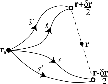
Figure 15: For fairly localized initial wave-packet, the four classical trajectories contributing to the LE can be reduced to those starting at its center $\mathbf{r}_{0}$.

$$f_{\Sigma}(\mathbf{r},t) =(4\pi\sigma^{2})^{d}\ \int\mathrm{d}\delta\mathbf{r}\ \sum_{s,s^{\prime}}\ \sum_{{\tilde{s}},{\tilde{s}}^{\prime}}\ \exp{\left[-\frac{(\mathcal{P}^{2}+\mathcal{S}^{2}+\mathcal{T}^{2})\sigma^{2}}{8\hbar^{2}}\right]}\exp{\left[-\frac{2\sigma^{2}}{\hbar^{2}}\left(\frac{\mathcal{R}}{4}-\mathbf{p}_{0}\right)^{2}\right]}$$

$$\times\ K_{s}\left(\mathbf{r}-\frac{\delta\mathbf{r}}{2},\mathbf{r}_{0};t\right)\ K_{s^{\prime}}^{\ast}\left(\mathbf{r}-\frac{\delta\mathbf{r}}{2},\mathbf{r}_{0};t\right)\ K_{{\tilde{s}}}^{\ast}\left(\mathbf{r}+\frac{\delta\mathbf{r}}{2},\mathbf{r}_{0};t\right)\ K_{{\tilde{s}}^{\prime}}\left(\mathbf{r}+\frac{\delta\mathbf{r}}{2},\mathbf{r}_{0};t\right)\ ,$$ (94)

with

$$\mathcal{S} ={\overline{\mathbf{p}}}_{s}-{\overline{\mathbf{p}}}_{s^{\prime}}+{\overline{\mathbf{p}}}_{{\tilde{s}}}-{\overline{\mathbf{p}}}_{{\tilde{s}}^{\prime}}\ ,$$ (95a)

$$\displaystyle\mathcal{T} ={\overline{\mathbf{p}}}_{s}+{\overline{\mathbf{p}}}_{s^{\prime}}-{\overline{\mathbf{p}}}_{{\tilde{s}}}-{\overline{\mathbf{p}}}_{{\tilde{s}}^{\prime}}\ .$$ (95b)

Given that

$$\mathcal{P}^{2}+\mathcal{S}^{2}+\mathcal{T}^{2}=\left({\overline{\mathbf{p}}}_{s}-{\overline{\mathbf{p}}}_{s^{\prime}}\right)^{2}+\left({\overline{\mathbf{p}}}_{s}-{\overline{\mathbf{p}}}_{{\tilde{s}}}\right)^{2}+\left({\overline{\mathbf{p}}}_{s}-{\overline{\mathbf{p}}}_{{\tilde{s}}^{\prime}}\right)^{2}+\left({\overline{\mathbf{p}}}_{s^{\prime}}-{\overline{\mathbf{p}}}_{{\tilde{s}}}\right)^{2}+\left({\overline{\mathbf{p}}}_{s^{\prime}}-{\overline{\mathbf{p}}}_{{\tilde{s}}^{\prime}}\right)^{2}+\left({\overline{\mathbf{p}}}_{{\tilde{s}}}-{\overline{\mathbf{p}}}_{{\tilde{s}}^{\prime}}\right)^{2}\ ,$$ (96)

and since the pairs of trajectories $(s,s^{\prime})$ and $({\tilde{s}},{\tilde{s}}^{\prime})$ have the same extreme points, the dominant contribution to $f_{\Sigma}$ will come from the terms with $s=s^{\prime}$ and ${\tilde{s}}={\tilde{s}}^{\prime}$. Such an identification minimizes the oscillatory phases of the propagators, and corresponds to the first diagonal approximation of the calculation of Sec. II and Ref. cit-Jalabert-Past, . Within such an approximation we have

$$f_{\Sigma}(\mathbf{r},t) =\left(\frac{\sigma^{2}}{\pi\hbar^{2}}\right)^{d}\ \int\mathrm{d}\delta\mathbf{r}\ \sum_{s,{\tilde{s}}}\ C_{s}\ C_{{\tilde{s}}}\ \exp{\left[-\frac{\left({\overline{\mathbf{p}}}_{s}-{\overline{\mathbf{p}}}_{{\tilde{s}}}\right)^{2}\sigma^{2}}{2\hbar^{2}}-\frac{2\sigma^{2}}{\hbar^{2}}\left(\frac{{\overline{\mathbf{p}}}_{s}+{\overline{\mathbf{p}}}_{{\tilde{s}}}}{2}-\mathbf{p}_{0}\right)^{2}\right]}$$

$$\exp{\left[\frac{\mathrm{i}}{\hbar}\left(\Delta S_{s}\left(\mathbf{r}-\frac{\delta\mathbf{r}}{2},\mathbf{r}_{0},t\right)-\Delta S_{{\tilde{s}}}\left(\mathbf{r}+\frac{\delta\mathbf{r}}{2},\mathbf{r}_{0},t\right)\right)\right]}\ ,$$ (97)

As in Eq. (14), $\Delta S_{s,{\tilde{s}}}$ is the extra contribution to the classical action that the trajectory $s$ (${\tilde{s}}$) acquires by effect of the perturbation $\Sigma$.

We have two different cases, depending on whether or not there are trajectories leaving from $\mathbf{r}_{0}$ with momentum close to $\mathbf{p}_{0}$ that arrive to the neighborhood of $\mathbf{r}$ after a time $t$. In the first case $\mathbf{r}$ is in the manifold that evolves classically from the initial wave-packet (Fig. 16). Such a contribution is dominated by the terms where the trajectory ${\tilde{s}}$ remains close to its partner $s$, and calling $f_{\Sigma}^{\mathrm{d}}$ this diagonal component, we get

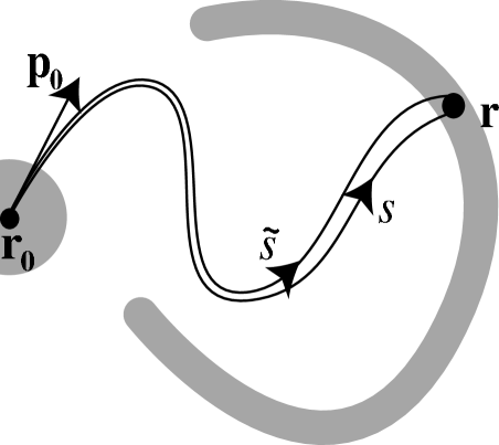
Figure 16: Classical trajectories in the manifold that evolves classically from $\mathbf{r}_{0}$ to $\mathbf{r}$, representing the diagonal component of $f_{\Sigma}$. The action differences $\Delta S$ of trajectories $s$ and ${\tilde{s}}$ are correlated. The shaded regions depict the initial and final classical densities.

$$f_{\Sigma}^{\mathrm{d}}(\mathbf{r},t)=\left(\frac{\sigma^{2}}{\pi\hbar^{2}}\right)^{d}\ \int\mathrm{d}\delta\mathbf{r}\ \sum_{s,{\tilde{s}}}\ C_{s}^{2}\ \exp\left[-\frac{2\sigma^{2}}{\hbar^{2}}\left({\overline{\mathbf{p}}}_{s}-\mathbf{p}_{0}\right)^{2}\right]\ \exp\left[\frac{\mathrm{i}}{\hbar}\left(\Delta S_{s}\left(\mathbf{r}-\frac{\delta\mathbf{r}}{2},\mathbf{r}_{0},t\right)-\Delta S_{{\tilde{s}}}\left(\mathbf{r}+\frac{\delta\mathbf{r}}{2},\mathbf{r}_{0},t\right)\right)\right]\ ,$$ (98)

Assuming, as in Sec. II and Ref. cit-Jalabert-Past, , that $\mathcal{H}_{0}$ stands for a chaotic system and that the perturbation $\Sigma$ represents a quenched disorder, upon average we obtain

$$\left\langle\exp\left[\frac{\mathrm{i}}{\hbar}\left(\Delta S_{s}\left(\mathbf{r}-\frac{\delta\mathbf{r}}{2},\mathbf{r}_{0},t\right)-\Delta S_{{\tilde{s}}}\left(\mathbf{r}+\frac{\delta\mathbf{r}}{2},\mathbf{r}_{0},t\right)\right)\right]\right\rangle=\exp\left[-\frac{1}{2\hbar^{2}}\ A\ \delta\mathbf{r}^{2}\right]\ ,$$ (99)

where $A$ is given by Eq. (34). We therefore have

$$f_{\Sigma}^{\mathrm{d}}(\mathbf{r},t)=\left(\frac{2\sigma^{4}}{\pi\hbar^{2}A}\right)^{d/2}\ \sum_{s(\mathbf{r}_{0},\mathbf{r},t)}\ C_{s}^{2}\ \exp{\left[-\frac{2\sigma^{2}}{\hbar^{2}}\left({\overline{\mathbf{p}}}_{s}-\mathbf{p}_{0}\right)^{2}\right]}\ ,$$ (100)

and the corresponding contribution to the Loschmidt echo is

$$M^{\mathrm{d}}(t)=\int d\mathbf{r}\ f_{\Sigma}^{\mathrm{d}}(\mathbf{r},t)=\left(\frac{2\sigma^{4}}{\pi\hbar^{2}A}\right)^{d/2}\ \int\mathrm{d}{\overline{\mathbf{p}}}\ C\exp{\left[-\frac{2\sigma^{2}}{\hbar^{2}}\left({\overline{\mathbf{p}}}-\mathbf{p}_{0}\right)^{2}\right]}\ .$$ (101)

As in Eqs. (13) and (27) we have used $C$ as the Jacobian of the transformation from $\mathbf{r}$ to ${\overline{\mathbf{p}}}$. Now the dominant trajectories are those starting from $\mathbf{r}_{0}$ and momentum $\mathbf{p}_{0}$. We are then back to the case of the previously discussed (Eqs. (35) and (72)) diagonal contribution.

$$M^{\mathrm{d}}(t)\simeq\overline{A}\ e^{-\lambda t},$$ (102)

where $C=(m/t)^{d}e^{-\lambda t}$ is assumed, and $\overline{A}=(m\sigma/A^{1/2}t)^{d}$. The decay rate of the diagonal contribution is set by the Lyapunov exponent $\lambda$, and therefore independent on the perturbation $\Sigma$.

The second possibility we have to consider is the case where there does not exist any trajectory leaving from $\mathbf{r}_{0}$ with momentum close to $\mathbf{p}_{0}$ that arrives to the neighborhood of $\mathbf{r}$ after a time $t$. It is a property of the Wigner function that in the region of phase space classically inaccessible by $X_{t}$ the points $\mathbf{r}$ half-way between branches of the classically evolved distribution will yield the largest values of $f_{\Sigma}$ (Fig. 17). The trajectories $s$ and ${\tilde{s}}$ visit now different regions of the configuration space, therefore the impurity average can be done independently for each of them. As in Eq. (24), we have

$$\left\langle\exp\left[\frac{\mathrm{i}}{\hbar}\Delta S_{s}\right]\right\rangle=\exp\left[-\frac{1}{2\hbar^{2}}\left\langle\Delta S_{s}^{2}\right\rangle\right]=\exp\left[-\frac{v_{0}t}{\widetilde{2\ell}}\right]_{.}$$ (103)

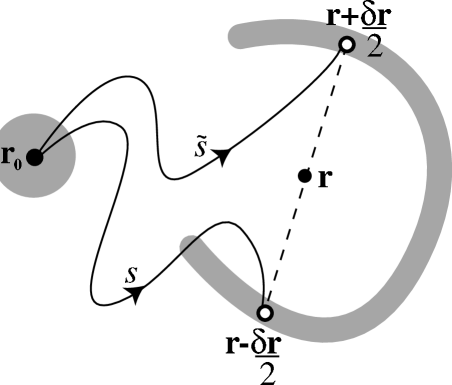
Figure 17: Non-diagonal classical contribution to the LE given by trajectories departing from $\mathbf{r}_{0}$ and arriving to points equidistant from the point $\mathbf{r}$ where the Wigner function is evaluated. The action differences $\Delta S$ associated with both trajectories are uncorrelated.

Such an average only depends on the length $L=v_{0}t$ of the trajectories. Thus, after average the non-diagonal term writes

$$f_{\Sigma}^{\mathrm{nd}}(\mathbf{r},t)=\left(\frac{\sigma^{2}}{\pi\hbar^{2}}\right)^{d}\exp\left[-\frac{v_{0}t}{\widetilde{\ell}}\right]\ \int\mathrm{d}\delta\mathbf{r}\ \sum_{s,{\tilde{s}}}\ C_{s}C_{{\tilde{s}}}\ \exp{\left[-\frac{\sigma^{2}}{\hbar^{2}}\left(\left({\overline{\mathbf{p}}}_{s}-\mathbf{p}_{0}\right)^{2}+\left({\overline{\mathbf{p}}}_{{\tilde{s}}}-\mathbf{p}_{0}\right)^{2}\right)\right]}\ .$$ (104)

The trajectory $s$ (${\tilde{s}}$) goes between the points $\mathbf{r}_{0}$ and $\mathbf{r}\mp\delta\mathbf{r}/2$. That is why the largest values of $f_{\Sigma}^{\mathrm{nd}}(\mathbf{r},t)$ are attained when $\mathbf{r}$ is in the middle of two branches of the classically evolved distribution. Other points $\mathbf{r}$ result in much smaller values of $f_{\Sigma}^{\mathrm{nd}}(\mathbf{r},t)$, since the classical trajectories that go between $\mathbf{r}_{0}$ and $\mathbf{r}\mp\delta\mathbf{r}/2$ require initial momenta ${\overline{\mathbf{p}}}_{s}$ (${\overline{\mathbf{p}}}_{{\tilde{s}}}$) very different from $\mathbf{p}_{0}$. Thus, exponentially suppressed contributions result.

The non-diagonal contribution to the Loschmidt echo can now be written as

$$M^{\mathrm{nd}}(t)=\int\mathrm{d}\mathbf{r}\ f_{\Sigma}^{\mathrm{nd}}(\mathbf{r},t)=\left(\frac{\sigma^{2}}{\pi\hbar^{2}}\right)^{d}\exp\left[-\frac{v_{0}t}{\widetilde{\ell}}\right]\ \left|\int\mathrm{d}\mathbf{r}\ \sum_{s}\ C_{s}\ \exp{\left[-\frac{\sigma^{2}}{\hbar^{2}}\left(\left({\overline{\mathbf{p}}}_{s}-\mathbf{p}_{0}\right)^{2}\right)\right]}\right|^{2}=\exp\left[-\frac{v_{0}t}{\widetilde{\ell}}\right]$$ (105)

As in Eqs. (27) and (60), we have made the change of variable from $\mathbf{r}$ to ${\overline{\mathbf{p}}}$, and accordingly, we have obtained the non-diagonal contribution to the LE cit-Jalabert-Past . As discussed before, such a contribution is a Fermi Golden Rule like cit-Jacquod01 . In the limit of $\hbar\rightarrow 0$ our diagonal term, Eq. (102), obtained from the final points who follow the classical flow, dominates the LE, consistently with our findings of Sec. IV.2.

V.3 Decoherence and emergence of classicality

Decoherence in a quantum system arises from its interaction with an external environment, over which the observers have no information nor control dissipation ; ZurekPT ; ZurekRMP . The states more sensitive to decoherence are those with quantum superpositions (Schrödinger cat states), since they depend strongly on the information coded in the phase of the wave-function, which is blurred by the interaction with the environment.

The studies of decoherence have traditionally considered one-dimensional systems, and often ignored the crucial role of its underlying classical dynamics hamburg . On the other hand, it has been proposed cit-Zurek-Paz and later corroborated numerically MonteolivaPaz , that for a classically chaotic system the entropy production rate (computed from its reduced density matrix) is given by the Lyapunov exponent. Moreover, as shown in Ref. cit-Jalabert-Past, and thoroughly discussed in this work, the decay rate of the Loschmidt echo in a multidimensional classically chaotic system becomes independent on the strength of the perturbation that breaks the time reversal between two well-defined limits (and set by the Lyapunov exponent). The connection between decoherence and Loschmidt echo has been discussed in Refs. cit-Jalabert-Past, ; preprintCDPZ, and has induced us to note as $\tau_{\phi}$ the relaxation rate of the LE.

Decoherence is typically analyzed through the time decay of the off-diagonal matrix elements of the reduced density matrix (where the environmental degrees of freedom of the total density matrix of the system and its environment are traced out), while the wave-function superposition defining the LE can be cast as a trace of reduced density matrices or Wigner functions evolving with different Hamiltonians (Eq. 2). Zurek has recently proposed to consider the relevance of sub-Planck structure (in phase-space) of the Wigner function for the study of quantum decoherence cit-ZurekNature . Considering the example of a coherent superposition of two minimum uncertainty Gaussian wave-packets (of width $\sigma$, centered at $\pm x_{0}$, and with vanishing mean momentum) in a one dimensional system, where the Wigner function (up to a normalization factor) is given by

$$W(x,p)=\exp\left[-\frac{(x-x_{0})^{2}}{\sigma^{2}}-\frac{\sigma^{2}p^{2}}{\hbar^{2}}\right]+\exp\left[-\frac{(x+x_{0})^{2}}{\sigma^{2}}-\frac{\sigma^{2}p^{2}}{\hbar^{2}}\right]+2\exp{\left[-\frac{x^{2}}{\sigma^{2}}-\frac{\sigma^{2}p^{2}}{\hbar^{2}}\right]}\cos\left[\frac{2px_{0}}{\hbar}\right]\ ,$$ (106)

it is clearly seen that in phase-space this distribution presents two spots located around $\pm x_{0}$ positive with positive values, and between them an oscillating structure taking large positive and negative values (called interference fringes for their similitude with a double-slit experience). It has then been proposed that the fringes substantially enhance the sensitivity of the quantum state to an external perturbation. A strong coupling with an environment suppresses the fringes, and the resulting Wigner function becomes positive everywhere and similar to the corresponding Liouville distribution of the equivalent classical system (with statistical mixtures instead of superpositions) ZurekRMP . Jacquod and collaborators cit-JacquodSP have contested this approach, by demonstrating that the enhanced decay is described entirely by the classical Lyapunov exponent, and hence insensitive to the quantum interference that leads to the sub-Planck structures of the Wigner function.

Working with the superposition of two Wigner functions (as in the case of the echo) and with genuinely multidimensional classically chaotic systems allows us to give a consistent description of the connection between quantum decoherence and the Loschmidt echo and the emergence of classical behavior.

In the previous sections, from the semiclassical evolution of the Wigner function we were able to identify the non-diagonal component $M^{\mathrm{nd}}$ as the contribution to the LE given by the values of the Wigner function between the branches of the classically evolved initial distribution (Fig. 17). Using the example of the two Gaussians of Eq. (106) (but keeping in mind that the situation is more complicated since our chaotic dynamics yields a much richer structure in phase-space), we see that in the region between branches both of the Wigner functions contributing to (2) are highly oscillating, and quite different from each other. The overlap, which is perfect for zero coupling (ensuring the unitarity requirement) is rapidly suppressed with increasing perturbation strength. As discussed earlier in the text (see also Refs. cit-Jalabert-Past ; cit-Jacquod01 ), when $M^{\mathrm{nd}}$ is the dominant contribution to $M$, we are in the Fermi Golden Rule regime. We have seen that this weak perturbation regime collapses as $\hbar\rightarrow 0$ (Eqs. 36 and 75).

Beyond a critical perturbation, the diagonal component $Md$ takes over as the dominant contribution to the LE, and is given by the values of the Wigner function on the regions of phase space that result from the classical evolution of the initial distribution. This is the Lyapunov regime, where the decay rate of $M(t)$ is given by $\lambda$. Notice that this behavior is still of quantum origin, as we are comparing the increase of the actions of nearby trajectories by the effect of a small perturbation, assuming that the classical dynamics is unchanged. The behavior in the Lyapunov regime does not simply follow from the classical fidelity, where the change in the classical trajectories is taken into account, and the finite resolution with which we follow them plays a major role. The upper value of the perturbation strength for observing the Lyapunov regime is a classical one, i.e. $\hbar$ independent ($\ell_{\mathrm{tr}}\simeq L$ in Sec. II.4 and Eq. (78)).

For stronger perturbations (see discussions in Sects. II.4 and IV.2) the classical trajectories are affected and the decay rate of the LE is again perturbation dependent. The Wigner function approach to the LE also helps to develop our intuition about the quantum to classical transition. The Lyapunov regime is the correct classical limit of a chaotic system weakly coupled to an external environment.

VI Conclusions

In this work we have studied the decay of the Loschmidt echo in classically chaotic systems and presented evidence for the universality of the Lyapunov regime, where the relaxation rate becomes independent of the perturbation, and given by the Lyapunov exponent of the classical system. Using analytical and numerical calculations we have determined the range (in perturbation strength) of the Lyapunov regime, its robustness respect to the classical limit, the form of the perturbation, and the average conditions.

We presented semiclassical calculations in two different Hamiltonian systems: a classically chaotic billiard perturbed by quenched disorder, and a Lorentz gas where the perturbation is given by an anisotropy of the mass tensor. In the later model, the numerical simulations were found in good agreement with the analytical calculations, and showed that the Lyapunov decay extends arbitrarily beyond the Ehrenfest time (where the quantum-classical correspondence is no longer expected to hold).

Using a Wigner function representation, we have been able to present an alternative interpretation of the two contributions to the Loschmidt echo. The non-diagonal (Fermi Golden Rule) regime obtained for weak perturbation was shown to arise from the destruction of coherence between non-local superpositions thus destroying the non-classical part of the distribution. In contrast, the diagonal (Lyapunov) regime obtained for stronger perturbation or more classical systems was shown to be given by the classical part of the evolved initial distribution. Thus, the Lyapunov regime is associated with the classical evolution (even though is of quantum origin), while the Fermi Golden Rule has a purely quantum nature. In this way, the persistence of the Lyapunov regime after Ehrenfest time is understood as the emergence of classical behavior due to the fast dephasing of the purely quantum terms. This is in consistency with the understanding of the quantum-classical transition in quantum systems coupled to an environment driven by the decoherence ZurekPT .

The existence and universality of an environment-independent regime and its consequence in the phase-space behavior of the Wigner function provide a highlight on the connection between the Loschmidt echo and quantum decoherence. Such a connection, as well as the experiments testing the universal behavior, are promising subjects for future research.

The universal behavior of the Loschmidt echo requires an underlying classically chaotic system, like the ones we have considered in this work. Hamiltonian systems with regular dynamics have been shown to exhibit an anomalous power-law for the decay of the Loschmidt echo cit-JacquodInt . This behavior is quite different from the one we obtain for chaotic systems. Therefore, we see that the Loschmidt echo constitutes a relevant concept in the study of Quantum Chaos cit-Bohigas . Such a connection, clearly deserves further studies.

The Loschmidt echo in the Lorentz gas has been recently calculated for short times GouDor , and a rate given by twice the Lyapunov exponent has been proposed. It would be interesting to investigate if the difference in times scales is responsible for the departure from our results.

Appendix A Classical dynamics with an anisotropic mass tensor

Let us assume a particle in a free space with mass tensor $\overset{\leftrightarrow}{m}$ surrounded by an infinite potential surface (hard wall). Suppose that the particle departs from a point $\mathbf{r}_{0}$ at time $t_{0}$ and arrives to a final point $\mathbf{r}$ at time $t$. We must calculate the time $t_{\mathrm{c}}$ and position $\mathbf{r}_{\mathrm{c}}$ along the surface at which the particle collides. The action along the trajectory is

$$S=\frac{(\mathbf{r}_{c}-\mathbf{r}_{0}){\overset{\leftrightarrow}{m}}(\mathbf{r}_{c}-\mathbf{r}_{0})}{2(t_{c}-t_{0})}+\frac{(\mathbf{r}-\mathbf{r}_{c}){\overset{\leftrightarrow}{m}}(\mathbf{r}-\mathbf{r}_{c})}{2(t-t_{c})}\ .$$ (107)

We can solve the problem by minimizing the action, taking the derivative of Eq. (107) along the surface. Introducing unitary vector $\mathbf{n}$ normal to the surface at the point of collision, we can express the minimization condition as

$$\mathbf{n}\times\nabla_{\mathbf{r}_{c}}S=0\ .$$ (108)

Denoting the initial and final velocities as $\mathbf{v}_{i}=(\mathbf{r}_{c}-\mathbf{r}_{0})/(t_{c}-t_{0})$ and $\mathbf{v}_{f}=(\mathbf{r}-\mathbf{r}_{c})/(t-t_{c})$, we can write

$$\mathbf{n}\times{\overset{\leftrightarrow}{m}}(\mathbf{v}_{i}-\mathbf{v}_{f})=0\ .$$ (109)

This, along with the conservation of energy $E=\mathbf{v}{\overset{\leftrightarrow}{m}}\mathbf{v}/2$, results in Eqs. (51). The same result is obtained in the case of stretched boundaries.

Appendix B Numerical method to simulate the quantum dynamics

In order to compute the quantum dynamics of the system we resort to a lattice discretization (tight-binding model) in a scale $a$ much smaller that the wavelength of the packets. This condition is relevant to accurately recover the dispersion relation of the free particle $E_{k}=\hbar^{2}k^{2}/(2m)$, from the energy spectrum of the (open boundaries) discretized system,

$$E_{k}=\frac{2\hbar^{2}}{ma^{2}}-\frac{\hbar^{2}}{ma^{2}}\left(\cos(k_{x}a)+\cos(k_{y}a)\right).$$ (110)

Setting the lattice step as the unit length ($a=1$) we typically worked with $R=20$, except for the calculations in Sec. IV.2 where, in order to keep the precision for smaller wavelengths, $a$ was reduced keeping the product $ka$ constant.

The discretization results in a Hamiltonian matrix whose diagonal elements are the on-site energies. The off–diagonal elements are hopping terms $V=\hbar^{2}/(2ma^{2})$ which is the maximum kinetic energy represented by the discretization.

The quantum dynamics on the lattice was carried out using a Trotter-Suzuki algorithm cit-DeRaedt , which is a remarkably precise and efficient numerical method. At the lowest order, it is a decomposition of the evolution operator $U$ for a small time $\tau$ in a product of analytically solvable evolution operators. Typically one searches for a way to write the Hamiltonian of the system as $\mathcal{H}=\sum_{k}^{Q}\mathcal{H}_{k}$, where $\mathcal{H}_{k}$ are $2\times 2$ matrices, and thus

$$U(\tau)=\exp{\left[\mathrm{i}\mathcal{H}\tau/\hbar\right]}\simeq\widetilde{U}(\tau)=\prod_{k}^{Q}\exp{\left[\mathrm{i}\mathcal{H}_{k}\tau/\hbar\right]}\ ,$$ (111)

where $U_{k}(\tau)=\exp[\mathrm{i}\mathcal{H}_{k}\tau/\hbar]$ are rotation matrices.

The highest orders involve a fractal decomposition of $\tau$ that preserves the unitarity of the approximated evolution operator. In our calculations, a fourth–order algorithm with a time step $\tau=0.1\hbar/V$ was precise enough for the time regime of interest.

References

- (1) R. Schuster et al., Nature 385, 417 (1997).
- (2) C. H. Bennet and D. P. DiVincenzo, Nature 404, 247 (2000).
- (3) E. L. Hahn, Phys. Rev. 80, 580 (1950); R. G. Brewer and E. L. Hahn, Sci. Am. 251, 50 (1984).
- (4) W. K. Rhim, A. Pines, and J. S. Waugh, Phys. Rev. Lett. 25, 218 (1970).
- (5) S. Zhang, B. H. Meier and R. R. Ernst, Phys. Rev. Lett. 69, 2149 (1992).
- (6) P. R. Levstein, G. Usaj and H. M. Pastawski, J. Chem. Phys. 108, 2718 (1998).
- (7) G. Usaj, H. M. Pastawski, P. R. Levstein, Mol. Phys. 95, 1229 (1998); H. M. Pastawski, G. Usaj and P.R. Levstein in Contemporary Problems of Condensed Matter Physics, edited by S. J. Vlaev, L. M. Gaggero Sager and V. V. Dvoeglazov, (NOVA Scientific Publishers, New York, 2001).
- (8) H. M. Pastawski, P. R. Levstein, G. Usaj, J. Raya and J. Hirschinger, Physica A 283, 166 (2000).
- (9) J. M. Ziman, Electrons and phonons: the theory of transport phenomena in solids (Clarendon Press, Oxford, 1962).
- (10) R. B. Laughlin, Nucl. Phys. B (Proc. Suppl.) 3, 213 (1987).
- (11) G. Casati, B. V. Chirikov, I. Guarneri and D. L. Shepelyansky, Phys. Rev. Lett. 56, 2437 (1986); F.M. Izrailev, Phys. Rep. 196, 299 (1990).
- (12) F. Haake, Quantum Signatures of Chaos (Springer-Verlag, Berlin, 1991).
- (13) O. Bohigas, M. J. Giannoni and C. Schmit, Phys. Rev. Lett. 52, 1 (1984).
- (14) E. J. Heller, Phys. Rev. Lett. 53, 1515 (1984).
- (15) A. Szafer and B. Altshuler, Phys. Rev. Lett. 70, 587 (1993).
- (16) A. Peres, Phys. Rev. A 30, 1610 (1984); A. Peres, in Quantum Chaos, edited by H. Cerdeira, R. Ramaswamy, M. C. Gutzwiller and G. Casati, (World Scientific, 1991).
- (17) M. A. Nielsen and I. L. Chuang, Quantum computation and quantum information (Cambridge University Press, Cambridge, New York, 2000).
- (18) R. A. Jalabert and H. M. Pastawski, Phys. Rev. Lett. 86, 2490 (2001).
- (19) W. H. Zurek and J. P. Paz, Phys. Rev. Lett. 72, 2508 (1994).
- (20) F. M. Cucchietti, H. M. Pastawski and R. Jalabert, Physica A 283, 285 (2000).
- (21) F.M. Cucchietti, H. M. Pastawski and D. A. Wisniacki, Phys. Rev. E 65, 045206(R) (2002).
- (22) Ph. Jacquod, P. G. Silvestrov, and C. W. J. Beenakker, Phys. Rev. E 64, 055203 (2001).
- (23) W. Wang and B. Li, Phys. Rev. E 66, 056208 (2002).
- (24) D. A. Wisniacki, E. G. Vergini, H. M. Pastawski and F. M. Cucchietti, Phys. Rev. E 65, 055206(R) (2002).
- (25) F. M. Cucchietti, C. H. Lewenkopf, E. R. Mucciolo, H. M. Pastawski, and R. O. Vallejos, Phys. Rev. E 65, 046209(R) (2002).
- (26) G. Benenti and G. Casati, Phys. Rev. E 65, 066205 (2002).
- (27) N. R. Cerruti and S. Tomsovic, Phys. Rev. Lett. 88, 054103 (2002).
- (28) T. Prosen, Phys. Rev. E 65, 036208 (2002).
- (29) T. Prosen and M. Znidaric, J. Phys. A 35,1455 (2002); T. Prosen, T. H. Seligman and M. Znidaric, quant-ph/0304104.
- (30) Ph. Jacquod, I. Adagideli and C. W. J. Beenakker, Europhys. Lett. 61, 729 (2003).
- (31) B. Eckhardt, J. Phys. A 36, 371 (2003).
- (32) G. Benenti, G. Casati, and G. Veble, Phys. Rev. E 67, 055202 (2003).
- (33) Y. Adamov, I. V. Gornyi, A. D. Mirlin, Rev. E 67, 056217 (2003).
- (34) G. P. Berman and G. M. Zaslavsky, Physica A 91, 450 (1978).
- (35) J. Vanicek and E. H. Heller, quant-ph/0302192.
- (36) W. H. Zurek, Nature 412, 712 (2001).
- (37) Z. P. Karkuszewski, C. Jarzynski and W. H. Zurek, Phys. Rev. Lett. 89, 170405 (2002).
- (38) D. Weiss et. al., Phys. Rev. Lett. 66, 2790 (1991).
- (39) D. Weiss et. al., Phys. Rev. Lett. 70, 4118 (1993).
- (40) A. Pouydebasque et. al., Phys. Rev. B 64, 245306 (2001).
- (41) Ph. Jacquod, I. Adagideli and C. W. J. Beenakker, Phys. Rev. Lett. 89, 154103 (2002).
- (42) M. C. Gutzwiller, Chaos in Classical and Quantum Mechanics (Springer-Verlag, NY, 1990); M.-J. Giannoni, A. Voros, and J. Zinn-Justin, eds. Chaos and Quantum Physics (North-Holland, Amsterdam, 1991).
- (43) M. Brack, Semiclassical Physics, Frontiers in Physics, Vol. 96 (Westview Press, 1997).
- (44) K. Richter, D. Ullmo, and R. A. Jalabert, Phys. Rev. B, 54, R5219 (1996).
- (45) K. Richter, D. Ullmo, and R. A. Jalabert, J. Math. Phys. 37, 5087 (1996).
- (46) R. A. Jalabert, in New Directions in Quantum Chaos, ed. by G. Casati, I. Guarneri and U. Smilansky (IOS Press, Amsterdam, 2000).
- (47) K. Richter, Semiclassical Theory of Mesoscopic Quantum Systems, Springer Trac. Mod. Phys. (Springer-Verlag, Berlin, 2000).
- (48) U. Weiss, Quantum Dissipative Systems (World Scientific, Singapore, 1993).
- (49) F.M. Cucchietti, C.H. Lewenkopf and H.M. Pastawski, unpublished.
- (50) As noticed in Ref. cit-SmoothBilliard, , the elastic mean-free path corresponding to a two-dimensional model of disorder used in Refs. cit-Jalabert-Past, ; RapComm, ; JMP, ; tstimp, ; hamburg, ; Kbook, should be affected by a factor of .
- (51) C. F. F. Karney, Physica D 8, 360 (1983); P. Grassberger and H. Kantz, Phys. Lett. A 113, 167 (1985).
- (52) V. I. Arnol’d, Mathematical methods of classical mechanics (Springer-Verlag, New York, 1978).
- (53) J. R. Dorfman An Introduction to Chaos in Nonequilibrium Statistical Mechanics (Cambridge Univ. Press, Cambridge, 1999).
- (54) I. L. Aleiner and A. I. Larkin, Phys. Rev. B 54, 14423 (1996).
- (55) P. Gaspard and G. Nicolis, Phys. Rev. Lett. 65, 1693 (1990).
- (56) H. van Beijeren and J. R. Dorfman, Phys. Rev. Lett. 74, 4412 (1995); idem 76, 3238 (1996).
- (57) G. Benettin, L. Galgani and J. M. Strelcyn, Phys. Rev. A 14, 2338 (1976).
- (58) H. M. Pastawski and G. Usaj, Phys. Rev. B 57, 5017 (1998).
- (59) R. Schack and C. M. Caves, Phys. Rev. E 53, 3387 (1996).
- (60) D. A. Wisniacki and D. Cohen, Phys. Rev. E 66, 046209 (2002).
- (61) P. G. Silvestrov, J. Tworzydlo, C. W. J. Beenakker, Phys. Rev. E 67, 025204(R) (2003).
- (62) A. M. Ozorio de Almeida, Phys. Rep. 295, 265 (1998).
- (63) F. Toscano and C. H. Lewenkopf, Phys. Rev. E 65, 036201 (2002).
- (64) H. M. Pastawski, Phys. Rev. B 46, 4053 (1992).
- (65) W. H. Zurek, Phys. Today 44, No 10, 36 (1991).
- (66) W. H. Zurek, Rev. Mod. Phys. 75, 715 (2003)
- (67) R. A. Jalabert and H. M. Pastawski, in Adv. in Solid State Phys., ed. by B. Kramer (Springer, Berlin, 2001).
- (68) D. Monteoliva and J.-P. Paz, Phys. Rev. Lett. 85, 3373 (2001).
- (69) F.M. Cucchietti, D. A. R. Dalvit, J.-P. Paz, and W. H. Zurek, quant-ph/0306142.
- (70) A. Goussev and J. R. Dorfman, nlin.CD/0307025.
- (71) H. De Raedt, Ann. Rev. Comp. Phys. IV, 107 (1996).