Quantum critical behavior of the one-dimensional ionic Hubbard model

Abstract

We study the zero-temperature phase diagram of the half-filled one-dimensional ionic Hubbard model. This model is governed by the interplay of the on-site Coulomb repulsion and an alternating one-particle potential. Various many-body energy gaps, the charge-density-wave and bond-order parameters, the electric as well as the bond-order susceptibilities, and the density-density correlation function are calculated using the density-matrix renormalization group method. In order to obtain a comprehensive picture, we investigate systems with open as well as periodic boundary conditions and study the physical properties in different sectors of the phase diagram. A careful finite-size scaling analysis leads to results which give strong evidence in favor of a scenario with two quantum critical points and an intermediate spontaneously dimerized phase. Our results indicate that the phase transitions are continuous. Using a scaling ansatz we are able to read off critical exponents at the first critical point. In contrast to a bosonization approach, we do not find Ising critical exponents. We show that the low-energy physics of the strong coupling phase can only partly be understood in terms of the strong coupling behavior of the ordinary Hubbard model.

I Introduction

I.1 Motivation

Theoretical studies of the ionic Hubbard model (IHM) date back as far as the early seventies (see Ref. Nagaosa, and references therein). The model consists of the usual Hubbard model with on-site Coulomb repulsion $U$ supplemented by an alternating one-particle potential of strength $\delta$. It has been used to study the neutral to ionic transition in organic charge-transfer saltsHubbard ; Nagaosa and to understand the ferroelectric transition in perovskite materials.Egami Based on results obtained from numericalSoos ; Resta and approximate methods,Strebel ; Ortiz it was generally believed that at temperature $T=0$ and for fixed $\delta$ a single phase transition can be found if $U$ is varied. This quantum phase transition was also interpreted as an insulator-insulator transition from a band insulator ($U\ll\delta$) to a correlated insulator ($U\gg\delta$). In the present paper, we discuss in detail how this transition occurs.

In 1999, Fabrizio, Gogolin, and Nersesyan used bosonization to derive a field-theoretical model which they argued to be the effective low-energy model of the one-dimensional IHM.Fabrizio Surprisingly, the authors found, using various approximations, that the field-theoretical model displays two quantum critical points as $U$ is varied for fixed $\delta$. For $U<U_{\text{c1}}$ the system is a band insulator (with finite bosonic spin and charge gaps), as expected from general arguments. At the first transition point $U_{\text{c1}}$, they found Ising critical behavior as well as metallic behavior in the sense that the gap to the bosonic charge modes goes to zero at the critical point only. In the intermediate regime, $U_{\text{c1}}<U<U_{\text{c2}}$, a spontaneously dimerized insulator phase (in which the bosonic spin and charge gaps are finite) with finite bond order (BO) parameter was found. The authors argued that the system goes over into a correlated insulator phase (in which the bosonic charge gap is finite) with vanishing bond order and bosonic spin gap at a second critical point $U_{\text{c2}}$ which is of Kosterlitz-Thouless (KT) type.

Several groups have attempted to verify this phase diagram for the IHM using mainly numerical methods. Variational and Green’s function Quantum Monte Carlo (QMC) data obtained for the BO parameter, the electric polarization, and the localization length were interpreted in favor of a scenario with a single critical point $U_{\text{c}}$ and finite BO for $U>U_{\text{c}}$.Wilkens In a different calculation using auxiliary field QMC, data for the one-particle spectral weight were argued to show two critical points with an intermediate metallic phase.Refolio Exact diagonalization studies of the Berry phaseTorio and energy gapsGidopoulos ; Pati ; Brune have been interpreted as favoring one critical pointPati or two points;Torio in two investigations this issue was left unresolved.Gidopoulos ; Brune Several density-matrix renormalization group (DMRG) studies have been performed focusing on different energy gaps, the localization length, the BO parameter, the BO correlation function, different distribution functions, and the optical conductivity. Takada ; Qin ; Brune ; Zhang Some of the results have been interpreted to be consistent with a two-critical-point scenario.Takada ; Qin ; Zhang In Ref. Brune, the signature of only one phase transition was found and the possible existence of a second transition was left undetermined. The phase diagram of the IHM has also been studied using approximate methods such as the self-consistent mean-field approximationCaprara ; Gupta ; Gros , the slave-boson approximation,Caprara and a real space renormalization group method.Gupta Although these studies led to interesting insights, the validity of the approximations in the vicinity of the critical region can be questioned on general grounds; therefore, we do not focus on these approaches any further here. The present situation can be summarized as being highly controversial.

Here we refrain from giving a detailed discussion of the merits and shortcomings of the various numerical methods used and the possible problems in interpretation of numerical results in the literature. Instead, we present a detailed study of the $T=0$ phase diagram of the one-dimensional IHM mainly based on DMRG calculations on systems with both open and periodic boundary conditions (OBC’s and PBC’s).

We have calculated a number of different many-body energy gaps, including the spin gap, the one-particle gap (the energy difference of the ground states with $N+1$, $N$, and $N-1$ electrons), and the gaps to the first (“exciton”) and second excited states. A definition of the gaps is given in Sec. II.1. Our results explicitly show that different gaps associated with charge degrees of freedom do not coincide in the thermodynamic limit, although they are often believed to in the literature (see also Refs. Qin, and Brune, ). Our data show that the exciton gap vanishes at a coupling which depends on $\delta$ and which we define as $U_{\text{c1}}$. At this critical point the spin gap remains finite. The spin gap vanishes at a second critical coupling, which defines our $U_{\text{c2}}$.

In addition to the energy gaps, we have determined the BO parameter and susceptibility as well as the charge-density-wave (CDW) order parameter. Since the single-site translational symmetry is explicitly broken due to the alternating potential, we will avoid using the term “order parameter” in describing the CDW order and instead use the term “ionicity” to refer to the difference in occupancy between sites on the two sublattices $\langle n_{A}-n_{B}\rangle$. We find that the ionicity is continuous and non-vanishing for all values of the interaction strength.

From the finite-size scaling of the BO parameter, we find a parameter regime with a non-vanishing dimerization starting at $U_{\rm c1}$ and ending at $U_{\rm c2}$. We find that the transitions at both critical points are continuous. The BO susceptibility shows one isolated divergence at $U_{\text{c1}}$ separated from a region of divergence starting at $U_{\text{c2}}$.

We have also investigated the electric susceptibility, which is finite in the thermodynamic limit for $U<U_{\text{c1}}$ and diverges at the lower transition point $U_{\text{c1}}$. For $U>U_{\text{c1}}$, the behavior is less clear: there seems to be a weak divergence with system size near $U_{\text{c2}}$ and for $U>U_{\text{c2}}$. This behavior is consistent with that of the density-density correlation function, which decays exponentially as expected in a band insulator phase for $U<U_{\text{c1}}$, but surprisingly decays as a power law with an exponent between 3 and 3.5 in the strong coupling regime, $U>U_{\text{c2}}$.

Using a scaling ansatz for the BO and the electric susceptibility we can determine the critical exponents at $U_{\text{c1}}$. In contrast to the bosonization approachFabrizio , we obtain critical exponents different from those of the two-dimensional Ising model.

For (almost) all observables, we find that a careful finite-size scaling analysis is crucial to obtain reliable results in the thermodynamic limit. Furthermore, since it is necessary to distinguish between fairly small, but finite, gaps and order parameters and vanishing ones, a detailed understanding of the accuracy of the DMRG data is essential.

In order to obtain a comprehensive picture of the ground-state phase diagram, we have studied the different phases (as a function of $U$) for different $\delta$’s which cover a wide range of the parameter space. We also consider the limit of large Coulomb repulsion $U\to\infty$ (for fixed $\delta$ and hopping matrix element $t$) and show that some aspects of the physics of the model in this limit can be understood in terms of an effective Heisenberg model, as has been suggested earlierNagaosa but has recently been questioned.Brune As a result of our investigations, we are able to resolve many of the controversial issues and present strong indications in favor of a scenario with two quantum critical points. At the appropriate points in the paper, we will briefly comment on the relationship of our results with the ones obtained in earlier publications.

The remainder of the paper is organized as follows. In Sec. I.2, we introduce the model and discuss the limits in which it can be treated exactly. In Sec. I.3, we discuss the details of our DMRG procedure. In Sec. II, our finite-size and extrapolated data for the energy gaps are discussed. In Sec. III, we present our results for the ionicity and show that in the large-$U$ limit they are consistent with analytical results obtained by mapping the IHM to an effective Heisenberg model. The BO parameter and the related susceptibility are investigated in Sec. IV.1. We present results for the electric susceptibility and the density-density correlation function in Sec. IV.2. In the numerical calculations of Secs. III to IV we use OBC’s, for which the DMRG algorithm performs best. To complete our DMRG study in Sec. V, we present results for the energy gaps calculated for PBC’s and summarize our findings in Sec. VI.

I.2 Model and exactly solvable limits

The one-dimensional IHM is given by the Hamiltonian

$$H = -t\sum_{j,\sigma}\left(c_{j\sigma}^{{\dagger}}c_{j+1\sigma}+\mbox{h.c.}\right)+U\sum_{j}n_{j\uparrow}n_{j\downarrow}$$ (1)

$$+\frac{\delta}{2}\sum_{j,\sigma}(-1)^{j}n_{j\sigma}\;,$$

where $c_{j\sigma}$ ($c_{j\sigma}^{{\dagger}}$) destroys (creates) an electron with spin $\sigma$ on lattice site $j$ and $n_{j\sigma}=c_{j\sigma}^{{\dagger}}c_{j\sigma}$. We set the lattice constant equal to 1 and denote the number of lattice sites by $L$. Here we study the properties of the half-filled system with $N=L$ electrons.

The system corresponds to the usual Hubbard model with an additional local alternating potential. It is useful to consider various limiting cases in order to gain insight into possible phases and phase transitions. For $U=0$ and $\delta>0$, the model describes a conventional band insulator with a band gap $\delta$. Since the alternating one-particle potential explicitly breaks the one-site translational symmetry, the ground state has finite ionicity.

The one-dimensional half-filled Hubbard model without the alternating potential ($\delta=0$) and with $U>0$ describes a correlated insulator with vanishing spin gap $\Delta_{\text{S}}^{\rm HM}(U)$ and critical spin-spin and bond-bond correlation functions.Voit All gaps associated with the charge degrees of freedom, such as the one-particle gap $\Delta_{1}^{\rm HM}(U)$, are finite.Florian (The gaps discussed here are defined in Sec. II.1.) The ionicity and the dimerization are zero for all values of $U$. These two limiting cases suggest that the system will be in two qualitatively different phases in the limits $U\ll\delta$ and $U\gg\delta$.

In the atomic limit, $t=0$, and for $0<U<\delta$, every second site of the lattice with on-site energy $-\delta/2$ (A sites) is occupied by two electrons while the sites with energy $\delta/2$ (B sites) are empty. The energy difference between the ground state and the highly degenerate first excited state is $\delta-U$. For $U>\delta$, both the A and B sites are occupied by one electron and the energy gap is $U-\delta$. Thus for $t=0$ a single critical point $U_{\text{c}}(\delta)=\delta$ with vanishing excitation gap can be found. One expects similar critical behavior with at least one critical point to persist for the full problem with finite $t$.

To describe the physics of the IHM in the limit $U\gg t,\delta$, an effective Heisenberg Hamiltonian

$$H_{\rm HB}=J\sum_{j}\left({\mathbf{S}}_{j}\cdot{\mathbf{S}}_{j+1}-\frac{1}{4}\right)\;,\;\;\;J=\frac{4t^{2}U}{U^{2}-\delta^{2}}$$ (2)

was derived in Ref. Nagaosa, analogously to the strong-coupling perturbation expansion of the usual Hubbard model. It has recently been pointed out that this strong-coupling mapping does not take into account an explicitly broken one-site translational symmetry.Brune However, it was shown in Ref. Nagaosa, that the strong-coupling expansion preserves the one-site translation symmetry in the effective spin Hamiltonian to all orders in the strong-coupling expansion. In addition, the ionicity can be derived directly from the effective spin Hamiltonian as follows. The symmetry of the Hamiltonian [Eq. (1)] implies that after taking the thermodynamic limit, $n_{j\sigma}=n_{j+2\sigma}$ for $\sigma=\uparrow,\downarrow$ and all $j$. Using the Hamiltonian Eq. (1) and the Hellman-Feynman theorem, the ionicity

$$\langle n_{A}-n_{B}\rangle=-\frac{2}{L}\sum_{j,\sigma}(-1)^{j}\langle n_{j\sigma}\rangle$$ (3)

can be determined via

$$\langle n_{A}-n_{B}\rangle=-\frac{4}{L}\left\langle\frac{\partial H}{\partial\delta}\right\rangle=-\frac{4}{L}\frac{\partial E_{0}}{\partial\delta}\;.$$ (4)

The ground-state energy $E_{0}$ of the effective Heisenberg model [Eq. (2)] is known analyticallyHBenergy and, in terms of $U$ and $\delta$, is given by

$$E_{0}^{\text{HB}}=L\frac{4Ut^{2}}{U^{2}-\delta^{2}}\left(\ln 2-\frac{1}{4}\right)$$ (5)

in the thermodynamic limit. In the limit $U\gg\delta$, we can thus derive an analytic expression for the ionicity

$$\langle n_{A}-n_{B}\rangle=32\ln 2\;\frac{U\delta t^{2}}{\left(U^{2}-\delta^{2}\right)^{2}}\;.$$ (6)

It implies that for any $U<\infty$, the ionicity of the IHM is nonzero and for large $U$ vanishes as $1/U^{3}$. Since CDW order is explicitly favored by the Hamiltonian, it is not surprising that the ionicity is non-vanishing for all finite $U$. As will be shown in Sec. III, this expression shows excellent agreement with our DMRG data for the IHM. This gives us confidence that the effective Heisenberg model indeed gives correctly at least certain aspects of the low-energy physics. Since the Heisenberg model [Eq. (2)] has a vanishing spin gap,HBzerospingap the mapping suggests that the spin gap also vanishes in the large-$U$ limit of the IHM.

Although the alternating potential breaks the one-site translational symmetry explicitly, the model remains invariant to a translation by two lattice sites. This leads to a site-inversion symmetry for closed-chain geometries with periodic or antiperiodic boundary conditions, a symmetry which is not present for OBC’s. As pointed out in Ref. Gidopoulos, , the ground state of the effective Heisenberg model with periodic boundary conditions for systems with $4n$ lattice sites or antiperiodic boundary conditions for systems with $4n+2$ sites has a parity eigenvalue of $-1$ whereas the ground state for $U=0$ has a parity eigenvalue of $+1$. This suggests that the IHM undergoes at least one phase transition point with increasing $U$ for fixed $\delta$. This level crossing will be replaced by level repulsion and approximate symmetries for other boundary conditions. In the thermodynamic limit, the effect of the boundaries will disappear and the level repulsion becomes vanishingly small. It is important to point out, however, that a level crossing on small finite systems does not necessarily lead to a first-order transition in the thermodynamic limit; careful finite-size scaling must be carried out in order to determine the critical behavior.

From these considerations, one expects to find at least one quantum phase transition from a phase with physical properties similar to those of a non-interacting band insulator to a phase with properties similar to those of the strong coupling phase of the ordinary Hubbard model. However, the details of the transition and the physical properties of the different phases remain unclear from these arguments. Furthermore, the behavior of the BO parameter in the critical region cannot be estimated from these simple limiting cases. Therefore, a detailed and careful calculation of the characterizing gaps and order parameters is necessary. Since no direct analytic approach is known to be able to treat the parameter values in the critical regime, we restrict ourselves to numerical calculations using the DMRG method with the details described in the next section.

In the following, we measure energies in units of the hopping matrix element $t$, i.e., set $t=1$. In order to be able to cover a significant part of the parameter space, we have carried out calculations with $\delta=1$, $\delta=4$, and $\delta=20$ for weak interaction values $U\ll\delta$, for strong coupling $U\gg\delta$ and in the intermediate critical regime $U\approx\delta$. For the sake of compactness, we will mostly focus on $\delta=20$ when presenting results that are generic to all three $\delta$-regimes.

I.3 DMRG method

We have carried out our calculations using the finite-system DMRG algorithm. Our investigation focuses on the ground-state properties for systems with OBC’s, i.e., we have performed DMRG runs mostly with OBC’s and one target state, the case in which the DMRG algorithm is most efficient. In order to perform the demanding finite-size scaling necessary, we have performed calculations for systems with up to $L=768$ sites, much larger than in an earlier work.Schoenhammer

In order to investigate the low-lying excitations, we have also performed calculations targeting up to three states simultaneously on systems with OBC’s. These numerically more demanding calculations were carried out for systems with up to $L=256$ sites for three target states and with up to $L=450$ sites for two target states. In order to compare with exact diagonalization calculations and to extend its finite-size scaling to larger systems, we have performed calculations for PBC’s with up to $L=64$ sites and one to three target states. In this case, the maximum system size is limited by the relatively poor convergence.

The DMRG calculations for OBC’s with one target state were carried out performing up to six finite-system sweeps keeping up to $m=800$ states. For more multiple states and for PBC’s up to 12 sweeps were performed, keeping up to $m=900$ states. In order to test the convergence of the DMRG runs, the sum of the discarded density-matrix eigenvalues and the convergence of the ground-state energy were monitored. For OBC’s, the discarded weight is of order $10^{-6}$ in the worst case and the ground-state energy is converged to an absolute error of $10^{-3}$ but in most cases the absolute error is $10^{-5}$ or better. This accuracy in both the energy and the discarded weight gives us confidence that the wave function is also well-converged and that local quantities are quite accurate.

For PBC’s, the discarded weight is of the order $10^{-5}$ in the worst case and the convergence of the ground-state energy for most runs is up to an absolute error of $10^{-3}$ or better, but for extreme cases such as $L=64$ and three target states for parameter values near the phase transition points, the convergence in the energy is sometimes reduced to an absolute error of only $10^{-1}$. However, we believe that this accuracy is high enough for the purposes of the discussion in section V.

In general, we find that our data are sufficiently accurate so that extrapolation in the number of states $m$ kept in the DMRG procedure does not bring about significant improvement in the results (at least for OBC’s). Details of the extrapolations and error estimates for particular calculated quantities are given in the corresponding sections.

II Energy gaps

One important way to characterize the different phases of the IHM are the energy differences between many-body eigenstates. Gaps to excited states can be used to characterize phases by making contact with the gaps obtained in bosonization calculations and also form the basis for experimentally measurable excitation gaps, found, for example, in inelastic neutron scattering, optical conductivity, or photoemission experiments. In addition to the gaps themselves, however, matrix elements between ground and excited states as well as the density of excited states are important in forming the full experimentally relevant dynamical quantities. An example is the matrix element of the current operator that comes into calculations of the optical conductivity. We have investigated the behavior of the matrix elements for the dynamical spin and charge structure factors and for the optical conductivity using exact diagonalization on systems with both PBC’s and OBC’s.

In the following, we present DMRG calculations of the gaps to first and second excited states, the spin gap, and the one-particle gap in which a careful finite-size scaling on systems of up to 512 sites is carried out. As we shall see, this is necessary in order to resolve the behavior of the gaps in the transition regime and to distinguish between scenarios with one or two critical points.

II.1 Definition of the gaps

In this section, we study excitations between a non-degenerate $S=0$ ground state and various excited states. In the numerical calculations, we have found that for OBC’s the ground state is non-degenerate with total spin $S=0$ for all parameter values studied here. We define the exciton gap

$$\Delta_{\text{E}}=E_{1}(N,S)-E_{0}(N,S=0)$$ (7)

as the gap to the first excited state in the sector with the same particle number $N$ and with $S_{z}=0$, where $S_{z}$ is the $z$-component of the total spin. We also calculate the expectation value of the total spin operator $\langle{\bf S}^{2}\rangle$ so that $S$ is known.

The spin gap is defined as the energy difference between the ground state and the lowest lying energy eigenstate in the $S=1$ subspace

$$\Delta_{\text{S}} = E_{0}(N,S=1)-E_{0}(N,S=0)\;.$$ (8)

When the first excited state $E_{1}(N,S)$ in the $S_{z}=0$ subspace is a spin triplet with $S=1$, $\Delta_{\text{S}}=\Delta_{\text{E}}$. Within the DMRG, this gap can be calculated by determining the ground-state energies in different $S_{z}$ subspaces in two different DMRG runs.

If $\Delta_{\text{E}}<\Delta_{\text{S}}$, we call the lowest excitation a charge excitation. In fact, exact diagonalization calculations for system with PBC’s suggest that the gap $\Delta_{\text{E}}$ corresponds to the gap in the optical conductivity.Brune We have carried out additional exact diagonalization calculations that show that the corresponding matrix elements of the current operator are also nonzero for OBC’s. We therefore expect that $\Delta_{\text{E}}$ (for excitations with $S=0$ and when $\Delta_{\text{E}}<\Delta_{\text{S}}$) corresponds to the optical gap in the thermodynamic limit.diploma To obtain a deeper understanding of the excitation spectrum in the critical region, we also calculate the gap to the second excited state

$$\Delta_{\text{SE}}=E_{2}(N,S)-E_{0}(N,S=0)$$ (9)

for selected parameters.

In the literature, gaps to excitations which can be classified as charge excitations are often calculated by taking differences between ground-state energies in sectors with different numbers of particles (this gap is commonly called the “charge gap”). In particular, one can define a $p$-particle gap

$$\Delta_{p} = \left[E_{0}(N+p,S^{z}_{\text{min}})+E_{0}(N-p,S^{z}_{\text{min}})\right.$$ (10)

$$\left.-2E_{0}(N,S=0)\right]/p$$

which is essentially the difference in chemical potential for adding and subtracting $p$ particles. The spin $S^{z}_{\text{min}}$ is the minimal value, 1/2 or 0 for $p$ odd and even, respectively. Either the one particle gap $\Delta_{1}$ or the two particle gap $\Delta_{2}$ are commonly used. The calculation of $\Delta_{1}$ or $\Delta_{2}$ is numerically less demanding than that of $\Delta_{\text{E}}$ since it is sufficient to calculate the ground-state energies in the subspaces with the corresponding particle numbers. However, since these gaps involve changing the particle number and, for $p=1$, the spin quantum number, it is not a priori clear if they can be used to characterize possible phase transition points of the $N$-particle system. In many cases of interest, the difference between $\Delta_{1}$, $\Delta_{2}$, and $\Delta_{\text{E}}$ vanishes for $L\to\infty$, but in other systems (an example is the Hubbard chain with an attractive interaction), their behavior differs. As we shall see, $\Delta_{1}$ and $\Delta_{\text{E}}$ do behave differently near $U_{\text{c1}}$. In this work we focus our investigation on $\Delta_{1}$. We have also calculated $\Delta_{2}$ and find that it behaves similarly to $\Delta_{1}$, although it generally takes on slightly larger values for finite systems.

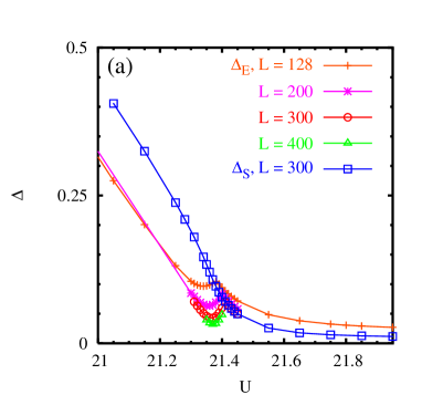
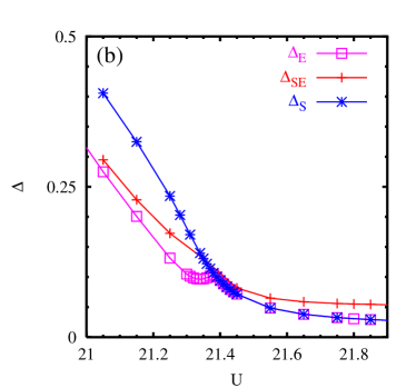
Figure 1: (a) The exciton gap $\Delta_{\text{E}}$ for finite system sizes $L$ and $\delta=20$. The spin gap $\Delta_{\text{S}}$ for $L=300$ is also shown for comparison. (b) The exciton gap, the spin gap $\Delta_{\text{S}}$ and the gap to the second excited state $\Delta_{\text{SE}}$ for $L=128$.

Gaps are also used to characterize the phase diagram within the bosonization approach.Fabrizio ; Brune It is generally believed that the bosonic charge gap defined there can be identified with the gap to the first excited state with spin quantum number $S=0$ (i.e. the exciton gap $\Delta_{\text{E}}$ [Eq. (7)] as long as $\Delta_{\text{E}}<\Delta_{\text{S}}$) and the bosonic spin gap with $\Delta_{\text{S}}$ [Eq. (8)], although a formal proof is missing.

Based on $\Delta_{\text{E}}$, $\Delta_{\text{S}}$, and $\Delta_{\text{SE}}$ and the very limited knowledge on matrix elements due to the small system sizes available to exact diagonalization, no reliable characterization of the metallic or insulating behavior of different phases and transition points can be given.

II.2 Gaps to excited states

In this section, we calculate excited states within the $S_{z}=0$ sector. Due to the additional numerical difficulty of calculating excited states in the same quantum number sector, we are restricted to systems of $L=450$ lattice sites for $\Delta_{\text{E}}$ and $L=256$ sites for $\Delta_{\text{SE}}$.

In Fig. 1(a), $\Delta_{\text{E}}$ as a function of $U$ is presented for $\delta=20$ and various $L$. For comparison, the spin gap for $L=300$ is also shown. The exciton gap develops a local minimum around $U=21.38$, which, for increasing $L$, becomes sharper. Furthermore, the value at the minimum becomes smaller and seems to approach zero. There is a cusp in $\Delta_{\text{E}}$ for all system sizes shown here at a certain $U$ to the right of the minimum, and then a smooth decay towards zero gap with further increasing $U$. As illustrated for $L=300$, this corresponds to a level crossing with the first triplet ($S=1$) excitation, which becomes the first excited state for all larger $U$ values, i.e., $\Delta_{\text{E}}=\Delta_{\text{S}}$. The data for $\delta=1$ and $\delta=4$ behave similarly, but the increase to the right of the minimum (up to the cusp) is substantially steeper as a function of $\delta$, so that it approaches a jump.

In Fig. 1(b), we display $\Delta_{\text{E}}$, the gap to the second excited state $\Delta_{\text{SE}}$, and the spin gap $\Delta_{\text{S}}$ (calculated using the ground state in the $S_{z}=1$ sector) for $L=128$. It can be seen that $\Delta_{\text{SE}}<\Delta_{\text{S}}$ for $U$-values to the left of the minimum in $\Delta_{\text{E}}$. A similar behavior is found for $\delta=4$ and $\delta=1$. This means that there is more than one $S=0$ excitation below the lowest lying $S=1$ excitation, consistent with a scenario in which a continuum of $S=0$ excitations becomes gapless at $U_{\text{c1}}$. This is the scenario predicted to occur at the first quantum critical point in the bosonization approach.Fabrizio Since system sizes for calculations of $\Delta_{\text{SE}}$ were limited to $L=128$ ($L=256$ for some parameter values), we did not attempt to systematically extrapolate $\Delta_{\text{SE}}$ to the thermodynamic limit.

We next discuss the finite-size scaling for $\Delta_{\text{E}}$ to the left of the cusp. For $U$ sufficiently far from the critical region (i.e., the minimum), the finite-size corrections are small and the data can safely be extrapolated to the thermodynamic limit using a quadratic polynomial in $1/L$, leading to a finite exciton gap. Close to the minimum, the scaling becomes more complicated. At smaller system sizes, we find $\Delta_{\text{E}}=\Delta_{\text{S}}$ and the scaling is nonlinear. However, at larger system sizes, there is a crossover to linear scaling with $\Delta_{\text{E}}(L)\neq\Delta_{\text{S}}(L)$. The crossover length scale becomes larger as $U$ approaches the position of the minimum. As a consequence, a reliable finite-size extrapolation in the critical region requires very large system sizes.

To investigate the behavior as $L\to\infty$, we interpolate $\Delta_{\text{E}}$ as a function of $U$ for fixed $L$ close to the minimum with cubic splines. From the interpolation we can read off the minimal value of the gap $\Delta_{\rm min}(L)$ and the position $U_{\rm min}(L)$ for the different system sizes. Fig. 2 shows the resulting $\Delta_{\rm min}(L)$ as a function of $1/L$ for $\delta=1$, $4$, and $20$. A linear extrapolation of the data gives $\Delta_{\rm min}(L=\infty,\delta=1)=3\times 10^{-3}$, $\Delta_{\rm min}(L=\infty,\delta=4)=5\times 10^{-4}$, and $\Delta_{\rm min}(L=\infty,\delta=20)=-1\times 10^{-4}$. Within the accuracy of our data and our extrapolation, these minimal gaps can be considered to be zero. In analogy with the atomic limit, we interpret the vanishing of the exciton gap as defining a critical point.Sachdev The critical coupling $U_{\text{c1}}$ can be determined from fitting $U_{\rm min}(L)$ to a linear function in $1/L$, as shown for $\delta=20$ in Fig. 3. The extrapolation is similar for the other $\delta$-values and we obtain $U_{\text{c1}}(\delta=1)\approx 2.71$, $U_{\text{c1}}(\delta=4)\approx 5.61$, and $U_{\text{c1}}(\delta=20)\approx 21.39$. As will be discussed in Sec. IV.2, the vanishing of the exciton gap is accompanied by a diverging electric susceptibility.

In Sec. IV.1, we will present strong evidence in favor of a spontaneously dimerized phase for $U_{\text{c1}}<U<U_{\text{c2}}$. Since the dimerized phase has an Ising-like symmetry, as $L\to\infty$ the ground state in this phase is expected to be two-fold degenerate and the exciton gap $\Delta_{\text{E}}$ is expected to vanish - at least if the thermodynamic limit is taken using PBC’s. At first glance this appears to be at odds with the increase of $\Delta_{\text{E}}$ as a function of $U$ to the right of $U_{\text{c1}}$ (but before the cusp is reached) as can be observed in Fig. 1(a). For finite systems, the OBC’s lift the degeneracy between the states with the two possible bond alternation patterns (strong, weak, strong, $\ldots$ and weak, strong, weak, $\ldots$), energetically favoring one of them which becomes the ground state. We have calculated the bond expectation values (see Sec. IV.1) of the ground state and the first excited state on systems of up to $L=450$ (the largest size we were able to reach) and find that the first excited state does not have the opposite alternation pattern. Instead, the alternation pattern is the same as in the ground state near the ends, but reverses itself in the middle of the chain. This change in the alternating BO parameter is evenly spread over the chain so that it has a cosine-like form with two nodes. It is difficult to perform finite-size extrapolation on $\Delta_{\text{E}}$ in this region since there are few system sizes and only a very limited range of $U$ available. However, one might speculate that $\Delta_{\text{E}}$ will remain finite as $L\to\infty$ due to the pinning of the BO parameter at the ends.

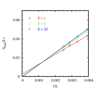
Figure 2: Finite-size scaling analysis of the minimal value of the exciton gap $\Delta_{\text{E}}$. The solid lines are linear fits through the four system sizes shown, $L=256$, 300, 350, 400.

Sufficiently far from $U_{\text{c1}}$, the data presented in Fig. 1(a) suggest a linear closing of the exciton gap, which gets rounded off in the critical region for finite systems. The larger $L$, the closer to $U_{\text{c1}}$ the deviation from linear behavior sets in. This suggests that $\Delta_{\text{E}}\sim U_{\text{c1}}-U$ close to but below the first critical point. It implies that the product of the critical exponents $z_{1}\nu_{1}=1$ at the first critical point,Sachdev where $z_{1}$ is the dynamical critical exponent and $\nu_{1}$ is the exponent associated with the divergence of the correlation length.

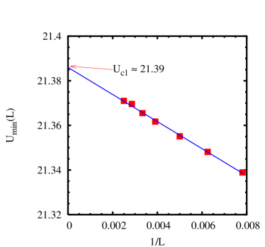
Figure 3: Finite-size scaling analysis of the $U$-value at the minimum of the exciton gap $\Delta_{\text{E}}$ for $\delta=20$. The solid line represents a linear least-squares extrapolation of the data yielding $U_{\text{c1}}\approx 21.39$.

Our finding of a vanishing exciton gap at the coupling $U_{\text{c1}}$ for OBC’s is consistent with results obtained using PBC’s and $L=4n$. For this case, a ground-state level crossing of two spin singlets at $U=U_{\text{x}}(L,\delta)$ (implying a zero exciton gap) was found using exact diagonalization of small systems.Gidopoulos ; Torio ; Brune A change of the site inversion symmetry at $U=U_{x}$ was also observed. In Sec. V, we will argue that $U_{\text{x}}(L\to\infty,\delta)$ coincides with $U_{\text{c1}}(\delta)$.Torio The presence of the ground-state level crossings might lead one to speculate that discontinuous behavior will persist in the thermodynamic limit, implying a first order phase transition at $U_{\text{x}}(L=\infty,\delta)$. However, we find no discontinuous behavior for systems with OBC’s, either on finite systems or in the $L\to\infty$ extrapolations. In order to agree with the results obtained for OBC’s in the thermodynamic limit, the discontinuous behavior for PBC’s must become progressively smoothed out as $L\to\infty$.

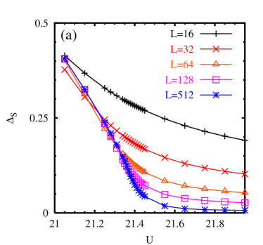
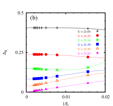
Figure 4: (a) The spin gap $\Delta_{\text{S}}$ for finite systems $L$ as a function of $U$ and (b) the finite-size scaling analysis for $\delta=20$ for chosen $U$-values. The system sizes $L=64$, 128, 200, 256, 300, 350, 400, 450, and 512 are shown in (b) and are used for a least-squares fit to a third-order polynomial in $1/L$ (solid lines). The dashed line in (b) shows the value of $\Delta_{\text{S}}$ at the largest system size in order to illustrate the non-monotonic behavior.

II.3 The spin gap $\Delta_{\text{S}}$

The spin gap $\Delta_{\text{S}}$ is shown in Fig. 4 as a function of $U$ for $\delta=20$ and system sizes between $L=16$ and 512. In Fig. 4(a), one can see that the spin gap systematically scales towards zero above a certain $U$ value. However, it is crucial that the finite-size scaling is carried out carefully and systematically in order to determine the behavior in the thermodynamic limit. As can be seen in the scaling as a function of $1/L$ for representative $U$ values in Fig. 4(b), and as was pointed out in Ref. Qin, , there is non-monotonic behavior as a function of $1/L$ for $U<U_{\text{c1}}$. In addition, the minimum of $\Delta_{\text{S}}$ as a function of $1/L$ shifts to larger system sizes as the critical region is approached. This makes an extrapolation to the thermodynamic limit in the critical region a difficult task which requires fairly large system sizes. In order to carry out an accurate extrapolation, we fit to a cubic polynomial in $1/L$.

Fig. 5 shows the extrapolated spin gap for $\delta=20$ presented together with the extrapolated values for $\Delta_{1}$ and $\Delta_{\text{E}}$. All three gaps are approximately equal for $U\ll U_{\text{c1}}$ (see the inset). Close to the transition, as can be seen on the expanded scale in the main plot, $\Delta_{\text{E}}$ goes to zero at $U_{\text{c1}}$, while $\Delta_{\text{S}}$ and $\Delta_{1}$ stay finite and are (almost; see below) equal. For $U>U_{\text{c1}}$, $\Delta_{\text{E}}$ increases until it reaches the spin gap $\Delta_{\text{S}}$. We find a region of $U>U_{\text{c1}}$ in which $\Delta_{\text{S}}(L=\infty)$ has a value that is clearly nonzero, well above the accuracy of the data which is of the order of the symbol size. The behavior is similar for $\delta=4$ (not shown). For even smaller values of $\delta$, $\Delta_{\text{S}}$ close to $U_{\text{c1}}$ becomes significantly smaller. As a consequence, the region in which $\Delta_{\text{S}}$ is non-vanishing for $U>U_{\text{c1}}$ is less pronounced at $\delta=1$. In this case, $\Delta_{\text{S}}$ at $U_{\text{c1}}$ is only a factor of six larger than the estimated accuracy of our data (this has to be compared to the factor of 20 for $\delta=4$ and 40 for $\delta=20$) with a fast decrease for $U>U_{\text{c1}}$. We take the estimate of accuracy from comparison of DMRG calculations for the one-particle gap of the usual 1D Hubbard model with Bethe ansatz results. We find that the difference is about $\left|\Delta_{1}^{\rm HM,DMRG}-\Delta_{1}^{\rm HM,exact}\right|=0.003$ in the worst case. We nevertheless interpret this small spin gap to be finite for $\delta=1$ and in a small region of $U\geq U_{\text{c1}}$. For $\delta$ substantially smaller than $1$, it is impossible to resolve a non-vanishing $\Delta_{\text{S}}$ at $U\geq U_{\text{c1}}$ using the DMRG.

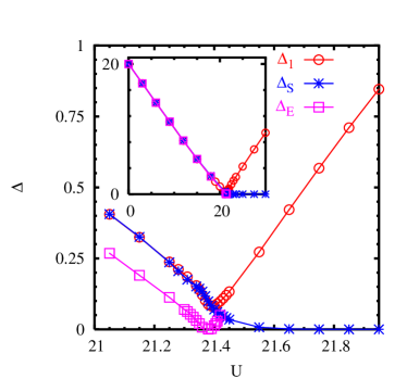
Figure 5: The exciton gap $\Delta_{\text{E}}$, the spin gap $\Delta_{\text{S}}$, and the one-particle gap $\Delta_{1}$ for $\delta=20$ after extrapolating to the thermodynamic limit $L\to\infty$. The inset shows the result for a larger range of $U$.

The spin gap data in Fig. 5 indicate that $\Delta_{\text{S}}$ goes to zero very smoothly between $21.55$ and $21.8$ and remains zero from there on. We here define $U_{\text{c2}}$ as the coupling at which $\Delta_{\text{S}}$ goes to zero. As we have argued in Sec. I.2, the mapping onto a Heisenberg model at strong coupling [Eq. (2)] suggests that the spin gap should vanish at sufficiently large $U$. However, we cannot strictly speaking exclude that $U_{\text{c2}}=\infty$ from the spin gap data. We give further evidence in support of two transition points at finite $U$ below.

Note that the extrapolated (Fig. 5) as well as the large-$L$ data (Fig. 4) for $\Delta_{\text{S}}$ display an inflection point in the vicinity of $U_{\text{c1}}$. This might be an indication of a non-analyticity related to the phase transition at $U_{\text{c1}}$.

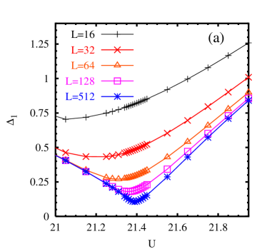
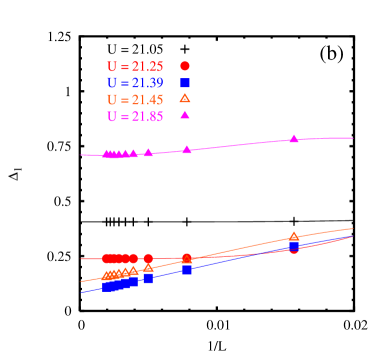
Figure 6: The one-particle gap $\Delta_{1}$ for $\delta=20$. (a) Results for finite systems with $L=16$ through 512. (b) The finite-size scaling behavior for $L=64$, 128, 200, 256, 300, 350, 400, 450, 512. The solid lines in (b) show least-squares fits to a third-order polynomial in $1/L$.

II.4 The one-particle gap $\Delta_{1}$

In Fig. 6(a), $\Delta_{1}$ as a function of $U$ is shown for $\delta=20$ and different $L$. Away from the critical region (which is between $U\approx 21.15$ and $U\approx 22$), the finite-$L$ data rapidly approach the thermodynamic limit and accurate results for $\Delta_{1}(L=\infty)$ can easily be obtained by fitting to a polynomial in $1/L$. Close to $U_{\text{c1}}$, the data for large $L$ develop a minimum. As $L$ increases, the position of the minimum shifts to larger $U$-values. The shape is quite rounded for the small system sizes, but becomes sharper for the largest sizes.

In the critical region, the finite-size scaling is again delicate. We examine $\Delta_{1}$ as a function of $1/L$ for a number of $U$-values near $U_{\text{c1}}$ for $\delta=20$ in Fig. 6(b). The data sufficiently away from the minimum (on both sites) shows linear behavior in $1/L$ for smaller system sizes, but then deviates from linear behavior and saturates at a finite value for larger $L$-values. This behavior is directly related to the $L$-dependence of the minimum of $\Delta_{1}$, which shifts to larger $U$ and becomes sharper with increasing system size. The scale on which a deviation from the linear behavior can be observed shifts to larger system sizes as $U$ approaches $U_{\text{c1}}$. In order to perform the finite-size scaling analysis, we fit to cubic polynomials in $1/L$, as we did for the spin gap. We have carried out this procedure for $\delta=1$ and $4$ and find that $\Delta_{1}(L,U)$ behaves similarly.

We have extracted the position and value at the minima by interpolating the data for fixed $L$ with cubic splines and then extrapolating to $L\to\infty$ with a fit to a quadratic polynomial. We obtain $U_{\text{min}}(\delta=1)\approx 2.71$, $U_{\text{min}}(\delta=4)\approx 5.63$, and $U_{\text{min}}(\delta=20)\approx 21.40$ for the positions and $\Delta_{1}(\delta=1,U_{\text{min}})\approx 0.02$, $\Delta_{1}(\delta=4,U_{\text{min}})\approx 0.05$, and $\Delta_{1}(\delta=20,U_{\text{min}})\approx 0.08$. The minimal values are finite to within the resolution of the data and the extrapolation, although the values are small, especially at small $\delta$. Therefore, $\Delta_{1}$ is finite in the critical region and is certainly larger than $\Delta_{\text{E}}$ which vanishes at $U_{\text{c1}}$. The positions of the minima are very close to, but at a slightly larger $U$-value than $U_{\text{c1}}$. The largest difference $U_{\text{min}}(\delta)-U_{\text{c1}}(\delta)$ turns out to be $0.02$ (for $\delta=4$). In Ref. Qin, , calculation were carried out for $\delta=0.6$ (in our units), this difference was found to be $0.04$, and $\Delta_{1}(\delta,U_{\text{min}})$ was concluded to be zero. The authors interpreted this as an indication of a second transition point (in addition to $U_{\text{c1}}$ which they determined from the vanishing of the exciton gap). While we have not carried out calculations at this value of $\delta$, our results suggest that $\Delta_{1}(\delta=0.6,U_{\text{min}})$ is (perhaps unresolvably) small, but nonzero. Therefore, we believe that $U_{\text{min}}$ is not associated with a second phase transition. In fact, as we have seen in Sec. II.3, the spin gap goes to zero at a substantially higher value of $U$ than $U_{\text{min}}$, and we associate this value with $U_{\text{c2}}$.

Up to a small difference (see Fig. 5) $\Delta_{1}(L=\infty)$ and $\Delta_{\text{S}}(L=\infty)$ are equal for $U<U_{\text{c1}}$. In fact, the values are virtually identical for the largest few system sizes and deviate only at smaller sizes. We therefore believe that the difference in the extrapolated gaps stems from differences in the fitting to the scaling function at smaller system sizes and that $\Delta_{1}(L=\infty)=\Delta_{\text{S}}(L=\infty)$ for $U<U_{\text{min}}\approx U_{\text{c1}}$ is consistent with our results. At this coupling, $\Delta_{1}(L=\infty)$ starts to become larger than $\Delta_{\text{S}}$ and as $U$ further increases, grows approximately linearly in $U$ as one would expect in a Mott insulator.

To summarize the behavior of the finite-size extrapolated gaps, we find that for $U\ll U_{\text{c1}}$, $\Delta_{\text{E}}=\Delta_{\text{S}}=\Delta_{1}$ as in a non-interacting band insulator. As $U_{\text{c1}}$ is approached, the gaps to two (or more) $S=0$ excitations drop below $\Delta_{\text{S}}$ and at least one of them goes to zero at $U_{\text{c1}}$. The one-particle gap $\Delta_{1}$ reaches a finite minimum around $U_{\text{c1}}$ and then increases (linearly for large $U$), and the spin gap $\Delta_{\text{S}}$ goes to zero smoothly at $U_{\text{c2}}>U_{\text{c1}}$. This smooth decay of the spin gap makes it difficult to quantitatively estimate $U_{\text{c2}}$. Since the above behavior is similar for the widely different potential strengths studied here, $\delta=1$, 4, and 20, we believe that it is generic for all $\delta$.

III Ionicity

As argued in Sec. I.2, the effective strong-coupling model (2) predicts that the ionicity $\langle n_{A}-n_{B}\rangle\sim 1/U^{3}$ for large $U$. For $t=0$, on the other hand, one expects a discontinuous jump from $\langle n_{A}-n_{B}\rangle=2$ to $\langle n_{A}-n_{B}\rangle=0$ at the single transition point $U_{\text{c}}$. Here we explore the behavior of $\langle n_{A}-n_{B}\rangle$ for all $U$ calculated within the DMRG.

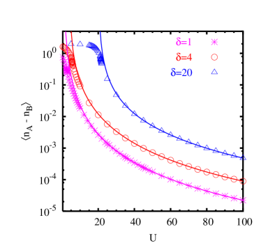
Figure 7: The ionicity $\langle n_{A}-n_{B}\rangle$ for $\delta=1,4,20$. The solid lines indicate analytical results from Eq. (6) and the symbols numerical DMRG results for $L=32$ sites.

In Fig. 7 we compare Eq. (6) for $\delta=1$, 4, 20 and various $U$ to results obtained from DMRG with OBC’s and $L=32$. By also considering larger system sizes (up to $L=512$) and PBC’s (up to $L=64$), we have verified that the $L=32$ results shown are already quite close to the thermodynamic limit for $U\gg\delta$. On the scale of the figure the difference between $L=32$ and $L=\infty$ is negligible. For large $U$, the DMRG data agree quite well with the analytical prediction, Eq. (6). This gives a strong indication that the large-$U$ mapping of the IHM onto an effective Heisenberg modelNagaosa is applicable at large but finite $U$. It is therefore tempting to conclude that $U_{\text{c2}}<\infty$. One should nevertheless keep in mind that the excellent agreement of the numerical data and the analytical prediction for the ionicity does not constitute a proof of this statement. We will return to this issue.

The DMRG data for $\langle n_{A}-n_{B}\rangle$ for $L=32$ shown in Fig. 7 are continuous as a function of $U$ for all $U$. We examine $\langle n_{A}-n_{B}\rangle$ more carefully as a function of system size in the vicinity of the first phase transition at $U_{\text{c1}}$ for $\delta=20$ in Fig. 8. The main plot shows DMRG data for various $L$ as a function of $U$ for $\delta=20$. While the data are continuous as a function of $U$ for all sizes, there is significant size dependence between $U=21.2$ and $21.5$, near the first critical point at $U_{\text{c1}}$. We have extrapolated the data to the thermodynamic limit using a second order polynomial in $1/L$ and have checked that other extrapolation schemes do not lead to significant differences in the extrapolated values. The $L=\infty$ extrapolated curve is shown in the inset. While the curve is still continuous, an inflection point can be observed close to $U_{\text{c1}}$. This might be related to non-analytic behavior at $U_{\text{c1}}$. We have found similar behavior of $\langle n_{A}-n_{B}\rangle$ for $\delta=1$ and $4$.

The behavior of $\langle n_{A}-n_{B}\rangle$ for PBC’s (and $L=4n$), which we have checked using the DMRG for up to $L=64$, is quite different. For finite $L$, the data display a jump discontinuity in the critical region which decreases in size for increasing $L$. The origin of this jump is the ground-state level crossing at $U_{\text{x}}(L,\delta)$. Since we do not observe any discontinuity in the ionicity calculated for OBC’s for $\delta=1$, 4, 20 and up to $L=512$, and since the jump obtained for PBC’s becomes smaller with system size, we expect that the jump vanishes in the thermodynamic limit and $\langle n_{A}-n_{B}\rangle$ becomes a continuous function.

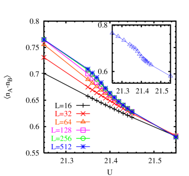
Figure 8: The ionicity $\langle n_{A}-n_{B}\rangle$ for finite systems with $L=16$, 32, $\ldots\;$, 512 for $\delta=20$. The inset shows the $L\to\infty$ extrapolated value.

IV Order parameters and susceptibilities

IV.1 The bond order parameter and susceptibility

The energy gaps have given us indications for two critical points. To study the nature of the intervening phase and the possibility of dimerization in more detail, we calculate the BO parameter

$$\left\langle B\right\rangle=\frac{1}{L-1}\sum_{j,\sigma}(-1)^{j}\left\langle c_{j+1\sigma}^{\dagger}c^{\phantom{{\dagger}}}_{j\sigma}+c_{j\sigma}^{\dagger}c^{\phantom{{\dagger}}}_{j+1\sigma}\right\rangle\;.$$ (11)

Since the OBC’s break the symmetry between even and odd bonds, $\left\langle B\right\rangle\neq 0$ for all finite systems. Therefore, a spontaneous dimerization can be obtained directly by extrapolating $\langle B\rangle$ to $L\to\infty$, i.e., without adding a symmetry-breaking field explicitly. One can form the corresponding BO susceptibility $\chi_{\rm BO}$ by adding a term

$$H_{\rm dim}=\rho\sum_{j,\sigma}(-1)^{j}\left(c_{j+1\sigma}^{\dagger}c^{\phantom{{\dagger}}}_{j\sigma}+c_{j\sigma}^{\dagger}c^{\phantom{{\dagger}}}_{j+1\sigma}\right)$$ (12)

to the Hamiltonian (1) and taking

$$\chi_{\rm BO}=\left.\frac{\partial\langle B\rangle(\rho)}{\partial\rho}\right|_{\rho=0}\;.$$ (13)

In practice, the derivative is discretized as $[\langle B\rangle(\rho)-\langle B\rangle(-\rho)]/(2\rho)$ where $\rho$ is taken to be small enough so that the system remains in the linear response regime.sizeoffieldamplitude Due to the additional symmetry breaking by the external dimerization field $\rho$, the DMRG runs converge more rapidly than in the $\rho=0$ case, making it easier to reach larger system sizes. Thus we were able to calculate $\chi_{\rm BO}$ on lattices of up to $L=768$ sites.

Fig. 9(a) shows $\left\langle B\right\rangle$ as a function of $U$ for $\delta=20$ and different $L$. The data develop a well-defined maximum near $U_{\text{c1}}$ for large $L$. The width of the “peak” for $L=512$ gives a first indication that there is a region in which the dimerization is non-vanishing. Typical results for the finite-size scaling of $\left\langle B\right\rangle$ are presented in Fig. 9(b). For $U\ll U_{\text{c1}}$, the data extrapolate linearly to zero in $1/L$. In the opposite limit, $U\gg U_{\text{c1}}$, we find $\left\langle B\right\rangle\sim 1/L^{\kappa}$ with $\kappa\approx 0.5-0.6$. A similar slow decay of the BO parameter has also been found in the standard and extended Hubbard models at half-filling.Eric The substantial finite-size corrections thus require very large systems to distinguish between scaling to zero with a slow power-law and scaling to a finite $L\to\infty$ limit. Below, but close to $U_{\text{c1}}$, the data for small $L$ initially display power-law-like finite-size scaling with $\kappa<1$, but for larger system size, one finds a crossover to a linear scaling of the BO parameter (to zero) as $L\to\infty$. There is also a crossover in the behavior for $U$-values near but above $U_{\text{c1}}$. One again finds a crossover from a power law with $\kappa<1$ for smaller system sizes to linear behavior that can be extrapolated to finite values of $\langle B\rangle_{\infty}$ for larger system sizes. The crossover length scale increases as $U$ approaches $U_{\text{c1}}$ until it becomes larger than the largest system size considered here. This length scale $L_{\text{c}}$ can be used to estimate the correlation length, which diverges at the first (continuous) critical point. We have been able to calculate $L_{\text{c}}$ for $U$-values on both sides of $U_{\text{c1}}$ and find that it diverges approximately linearly in $|U-U_{\text{c1}}|$. This implies $\nu_{1}=1$ (see also below). Taking into account that $z_{1}\nu_{1}=1$ as extracted from the linear closing of $\Delta_{\text{E}}$, one finds $z_{1}=1$ for the dynamical critical exponent.

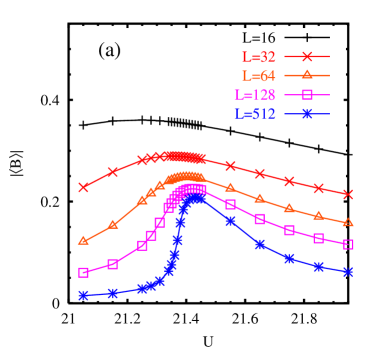
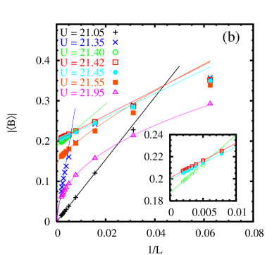
Figure 9: (a) The bond order parameter $\langle B\rangle$ for $\delta=20$ for finite systems as a function of $U$ for various system sizes. (b) The scaling of the data as a function of the inverse system size $1/L$. The solid lines are least-squares fits to the data as described in the text. The inset shows an expanded view of the scaling for $U$ values near the critical point.

This diverging crossover length scale makes it essential to treat system sizes that are significantly larger than the scale $L_{\text{c}}$, even close to the critical point $U_{\text{c1}}$. In order to obtain reliable results, we have calculated $\langle B\rangle_{L}$ for a number of system sizes $L>200$. In carrying out the finite-size extrapolation, we fit to a linear form for the largest system sizes if it is clear that $L_{\text{c}}$ has been reached, as can be seen in the inset of Fig. 9(b).

In Fig. 10, the finite-size extrapolation $\left\langle B\right\rangle_{\infty}$ is shown as a function of $U$ for $\delta=1$, 4, and 20. As can be seen, $\left\langle B\right\rangle_{\infty}=0$ to well within the error of the extrapolation for $U<U_{\text{c1}}$. For $U>U_{\text{c1}}$, we find a region of width between 0.2 and 0.4 (i.e., a factor of 5 to 10 larger than the extent of the dimerized phase claimed to be found in Ref. Qin, ) in $U$ in which $\left\langle B\right\rangle_{\infty}$ is distinctly finite. The onset of finite $\left\langle B\right\rangle_{\infty}$ at $U_{\text{c1}}$ is rather steep for all three values of $\delta$, but seems to be continuous. This steep onset suggests a critical exponent of the order parameter that is substantially smaller than 1. Within bosonization the first critical point was predicted to be Ising-like with $\beta_{1}=1/8$.Fabrizio The fall-off to zero as $U$ increases, on the other hand, is slow, with a small or vanishing slope. This behavior would be consistent with a second critical point at which the critical exponent for the order parameter is larger than one or at which a higher order phase transition such as a Kosterlitz-Thouless transition takes place.Fabrizio As can be seen by comparing Fig. 10(a), (b), and (c), the height of the maximum increases with increasing $\delta$. For $\delta$ significantly smaller than 1, the BO parameter is so small that it cannot be concluded to be finite within the numerical accuracy of the DMRG. For the couplings at which the finite dimerization sets in we obtain $U_{\text{c1}}(\delta=20)\approx 21.39$ and $U_{\text{c1}}(\delta=4)\approx 5.61$, which are in excellent agreement with the results obtained from the vanishing of $\Delta_{\text{E}}$. The value obtained for $\delta=1$, $U_{\text{c1}}(\delta=1)\approx 2.67$, is also in reasonably good agreement with the results obtained from the analysis of the gaps.

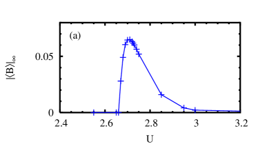
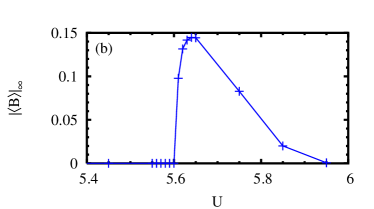
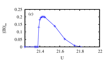
Figure 10: The bond-order parameter $\langle B\rangle_{\infty}$ in the thermodynamic limit for (a) $\delta=1$, (b) $\delta=4$, and (c) $\delta=20$ plotted as a function of $U$ near the transition points.

While our data suggest that a critical coupling $\tilde{U}_{\text{c2}}$, with $\left\langle B\right\rangle_{\infty}=0$ for $U>\tilde{U}_{\text{c2}}$, exists, no reliable quantitative estimate of $\tilde{U}_{\text{c2}}$ can be given based on the DMRG data for the BO parameter. Due the close proximity of the two critical points, we were not able to obtain quantitative results for the critical exponents $\beta_{1}$ and $\beta_{2}$ at the critical points, either by a direct fit of the $L=\infty$ results or by a scaling plot of the finite-size data. As discussed next, accurate exponents at $U_{\text{c1}}$ can be extracted from both the BO and the electric susceptibilities, and a more accurate estimate of $\tilde{U}_{\text{c2}}$ can be obtained from the BO susceptibility.

In order to understand the behavior of the BO susceptibility, it is useful to first examine the behavior of the BO parameter $\langle B\rangle$ as a function of the applied dimerization field $\rho$. This quantity is shown in Fig. 11 for $\delta=20$, three representative values of $U$, and different system sizes. For $U=19<U_{\text{c1}}$, the system is in a phase with vanishing BO parameter, and the slope at $\rho=0$ remains finite for all system sizes, corresponding to a finite susceptibility. The value $U=21.42$ is in the intermediate regime where we have found a finite BO parameter in the thermodynamic limit. As can be seen in the main part of the figure, a jump in $\langle B\rangle(\rho)$ develops. As the system size increases, the absolute value of dimerization field at which the jump occurs becomes smaller. This is the behavior expected in a dimerized phase in a system with OBC’s. Therefore, the jump in $\langle B\rangle(\rho)$ provides additional evidence in support of an intermediate phase with finite dimerization. For the approximate calculation of the susceptibility $\chi_{\rm BO}\approx[\langle B\rangle(\rho)-\langle B\rangle(-\rho)]/(2\rho)$, we have taken $\rho=10^{-4}$ which is small enough to stay to the right of the jump for all system sizes considered. Finally, for $U=50\gg U_{\text{c2}}$, $\langle B\rangle(\rho)$ goes to zero for $|\rho|\to 0$ and increasing system size indicating a phase without spontaneous dimerization. However, the slope at small $|\rho|$ becomes steeper with increasing system size, indicating a divergence of $\chi_{\text{BO}}$.

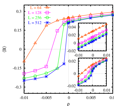
Figure 11: The BO parameter $\langle B\rangle$ as a function of applied dimerization field $\rho$ for $\delta=20$ and $U=21.42$. The upper inset shows data for $U=19$ and the lower inset data for $U=50$.

In Fig. 12, the BO susceptibility as a function of $U$ is shown for $\delta=1$, 4, 20 and different $L$. For all $\delta$ values, one observes a two-peak structure that becomes progressively more well-defined with increasing system size. There is a narrow peak at a $U$-value that agrees well with $U_{\text{c1}}$ determined earlier whose height grows rapidly with system size. It signals the onset of spontaneous dimerization. For somewhat larger $U$ there is a minimum in $\chi_{\text{BO}}$, surrounded by narrow region in which its value seems to saturate with system size. For still larger $U$-values, a second, broad peak develops. The position of this second maximum is roughly at $\tilde{U}_{\text{c2}}$, the $U$-value at which the BO parameter vanishes. We argue that the second peak is related to the second phase transition from the dimerized phase into an undimerized phase. To the right of the second peak, $\chi_{\text{BO}}$ does not seem to saturate for increasing system size, implying that $\chi_{\text{BO}}$ is divergent for all $U\geq U_{\text{c2}}$. One can understand this divergent behavior by studying the BO susceptibility for the ordinary Hubbard model $\chi_{\text{BO}}^{\rm HM}$. One finds that $\chi_{\text{BO}}^{\rm HM}$ is divergent for all $U>0$ because the bond-bond correlation function is critical.Voit A finite-size extrapolation of $\chi_{\text{BO}}$ is shown in Fig. 13 for large $U$-values for both $\delta=0$ and $\delta=20$. We find a power law divergence, $\chi_{\text{BO}}(L)\sim L^{\zeta}$, with $\zeta\approx 0.68$ for the ordinary Hubbard model and $\zeta\approx 0.65$ for the IHM. These values are in good agreement, considering the accuracy of the fit and additional finite-size effects.

Since $\chi_{\text{BO}}$ diverges for all $U$ to the right of the second peak, it is difficult to accurately determine the critical coupling $\tilde{U}_{\text{c2}}$. However, two different ways of estimating $\tilde{U}_{\text{c2}}(\delta)$ under- and overestimate its value. In the first method, $\tilde{U}_{\text{c2}}$ is estimated as the lowest $U$-value for which $\chi_{\text{BO}}$ seems to diverge for increasing $L$ and the available system sizes. It is then still possible that there is a crossover above a length scale unreachable by us and $\chi_{\text{BO}}$ scales to a finite value.

This tends to underestimate $\tilde{U}_{\text{c2}}$. In the second method, $\tilde{U}_{\text{c2}}$ is taken to be the position of the second peak at fixed $L$, extrapolated to $L\to\infty$. Since the peak position decreases for increasing $L$, this method tends to overestimate $\tilde{U}_{\text{c2}}$. From these two procedures, we obtain the bounds $21.55<\tilde{U}_{\text{c2}}(\delta=20)<21.69$. For the other values of $\delta$, it is very difficult to accurately determine the lower bound with the data available. We therefore only give the upper bound $\tilde{U}_{\text{c2}}(\delta=1)<2.95$ and $\tilde{U}_{\text{c2}}(\delta=4)<5.86$.

It is generally believed that a quantum critical point is accompanied by a vanishing characteristic energy scale.Sachdev At $\tilde{U}_{\text{c2}}$ the most obvious candidate is $\Delta_{\text{S}}$, consistent with our numerical data (see Figs. 4 and 5) and implying that $\tilde{U}_{\text{c2}}=U_{\text{c2}}$. This is assumed in the following discussion.

Since the peak in $\chi_{\text{BO}}$ at $U_{\text{c1}}$ is well-defined and has a clear growth with system size, it is reasonable to perform a finite-size scaling analysis. We use a scaling ansatz of the form

$$\chi(U,L)=L^{2-\eta}\tilde{\chi}(L/\xi)\;,$$ (14)

with $\xi\sim|U-U_{\text{c}}|^{-\nu}$. As can be seen in Fig. 12(d), data for $\delta=20$ and system sizes of $L=128$ and greater collapse onto one curve. The best fit is obtained with $U_{\text{c1}}=21.385$ and the critical exponents $\eta_{1}=0.45$ and $\nu_{1}=1$. The latter value is consistent with the value $\nu_{1}=1$ extracted from the divergence of the length scale discussed above. Note that the value of $\eta_{1}$ is not in agreement with the value expected in the two-dimensional Ising transition, $\eta=1/4$.Fabrizio We have also applied the scaling ansatz for $\delta=1$ and $4$. For decreasing $\delta$, the quality of the collapse of the data for the available systems sizes becomes poorer and the extracted exponents therefore become less reliable. The best fit is again obtained with $\nu_{1}=1$ for both $\delta$, $\eta_{1}(\delta=4)\approx 0.55$ and $\eta_{1}(\delta=1)\approx 0.65$. For the critical coupling we obtain $U_{\text{c}1}(\delta=1)\approx 2.7$ and $U_{\text{c}1}(\delta=4)\approx 5.6$, in excellent agreement with the values found by other means.

It is also possible to collapse the finite-size data onto one curve at the second transition point using the scaling ansatz (14). We find that the best results are obtained for $\xi\sim\exp(A/(U-U_{\text{c2}}^{\prime})^{B})$, indicating that the divergence of the susceptibility at $U_{\text{c2}}$ may indeed be exponential as expected for a KT-like transition. However, fitting the limited amount of data available to this form does not produce completely unambiguous results for all fit parameters.

Therefore, we have not further attempted to obtain results for $A$, $B$, $U_{\text{c2}}^{\prime}$, and $\eta_{2}$ with this method.

IV.2 The electric susceptibility and the density-density correlation function

In order to further investigate the physical properties of the different phases and transition points, we calculate the electric polarization and susceptibility.Aebischer The polarization is given by

$$\left\langle P\right\rangle=\frac{1}{L}\sum_{j}x_{j}\left\langle n_{j\uparrow}+n_{j\downarrow}\right\rangle\;,$$ (15)

where $x_{j}=j-L/2-1/2$ is the position along the chain, measured from the center. The polarization is the reponse due to a linear electrostatic potential

$$H_{\rm el}=-E\sum_{j}x_{j}\left(n_{j\uparrow}+n_{j\downarrow}\right)$$ (16)

which is added to the Hamiltonian (1). The electric susceptibility

$$\chi_{\text{el}}\;=\;\left.\frac{\partial\langle P\rangle(E)}{\partial E}\right|_{E=0}$$ (17)

is the susceptibility associated with this field.

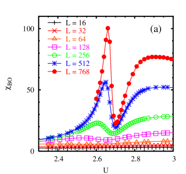
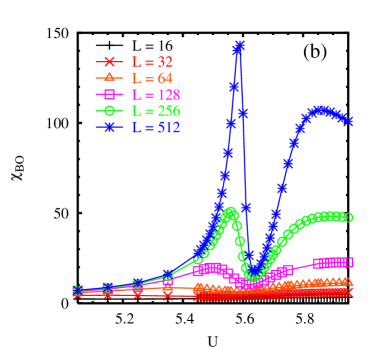
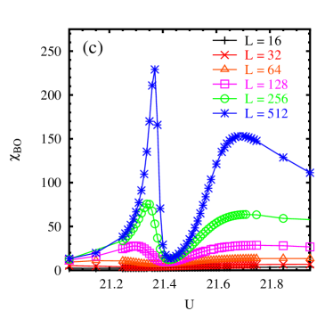
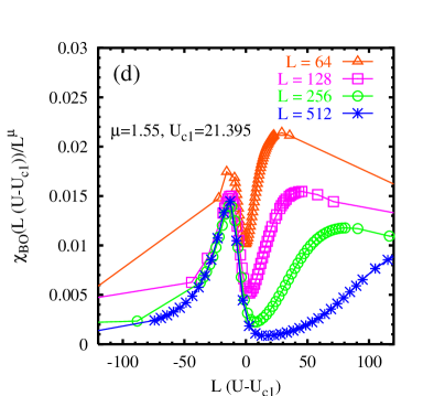
Figure 12: The BO susceptibility $\chi_{\text{BO}}$ as a function of $U$ for (a) $\delta=1$, (b) $\delta=4$, and (c) $\delta=20$ and different $L$. (d) A scaling analysis of the $\delta=20$ data from (c).

The electric susceptibility has been used to investigate the metal-insulator transition in the $t$-$t^{\prime}$-Hubbard model.Aebischer

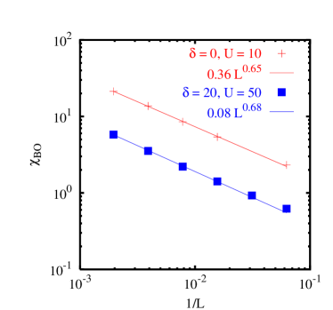
Figure 13: The BO susceptibility $\chi_{\text{BO}}$ as a function of $1/L$ for the ordinary Hubbard model ($\delta=0$) and $U=10$ and the ionic Hubbard model for $\delta=20$ and $U=50$. DMRG data are indicated by the corresponding symbols and the solid curves represent a least-squares fit to the indicated forms.

In this model, both a phase in which $\chi_{\text{el}}$ diverges as $L^{2}$ (a perfect metal) and a phase in which for increasing system size $\chi_{\text{el}}$ scales to a finite value (an insulator) were found when varying $U$ for fixed nearest-neighbor hopping $t$ and next-nearest-neighbor hopping $t^{\prime}$.

In contrast to the ordinary Hubbard model, the polarization does not always vanish at field $E=0$ in the IHM. For $U=0$, $\delta>0$, one finds $\left\langle P\right\rangle=-1/2$. This is due to the alternating ionic potential which induces a charge displacement to the sites with lower potential energy. Due to the OBC’s, a chain with even length $L$ starts and ends with a different potential, inducing a dipole moment. This is a boundary effect. In the strong coupling limit, $U\gg\delta$, we find that $\left\langle P\right\rangle\to 0$, as expected. The electric suceptibility $\chi_{\text{el}}$ can be calculated by discretizing the derivative as $[\langle P\rangle(E)-\langle P\rangle(E=0)]/E$. The field $E$ must be taken to be small enough so that the system remains in the linear response regime.sizeoffieldamplitude Note that it is necessary to subtract $\langle P\rangle(E=0)$ since it is nonzero in general.

A plot of $\chi_{\text{el}}$ as a function of $U$ for various system sizes is shown in Fig. 14(a) for $\delta=20$. For $U\ll U_{\text{c1}}$ and increasing $L$, $\chi_{\text{el}}$ converges to a finite value, similar to the behavior in a non-interacting band insulator and in the correlated insulator phase of the $t$-$t^{\prime}$-Hubbard model.Aebischer The data clearly develop a maximum at $U_{\text{c1}}$ whose height increases markedly with system size, indicating a divergence at the first critical point. The finite-size scaling of this height is consistent with a power-law increase, $L^{2-\eta_{1}}$, with $\eta_{1}\approx 0.46$. This increase is weaker than the $L^{2}$ divergence (which implies $\eta=0$) found in Ref. Aebischer, and associated with a perfect metal. For $U$ slightly larger than $U_{\text{c1}}$, the data again seem to saturate with system size. Assuming the scaling form of Eq. (14), the data close to $U_{\text{c1}}$ can be collapsed on a single curve as demonstrated in Fig. 14(b). The best fit is obtained for $\nu_{1}=1$ and $\eta_{1}\approx 0.45$. Both of these exponents are in excellent agreement with those found in the scaling analysis for $\chi_{\rm BO}$. We have carried out a finite-size scaling analysis for $\delta=4$ and $\delta=1$ and also find diverging peaks at $U_{\text{c1}}$, as well as collapse of the data onto a single curve using the scaling form (14) with exponents $\eta_{1}(\delta=1)=0.52$, $\eta_{1}(\delta=4)=0.45$, and $\nu_{1}=1$ (for both $\delta$). The critical $U$-values obtained from this scaling procedure are $U_{\text{c1}}(\delta=1)=2.68$, $U_{\text{c1}}(\delta=4)=5.59$, and $U_{\text{c1}}(\delta=20)=21.38$, which compare well to the values for the critical coupling obtained from the gaps and from the BO parameter and susceptibility.

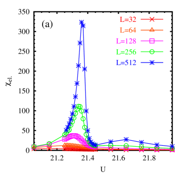
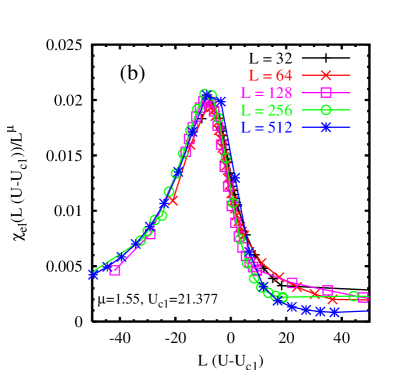
Figure 14: (a) The electric susceptibility $\chi_{\text{el}}$ for $\delta=20$ plotted as a function of $U$. (b) A scaling analysis of the data of (a).

The data for $\delta=20$ and $\delta=4$ for the largest system sizes, $L=256$ and $L=512$, suggest that a second peak may develop around $U_{\text{c2}}$. In order to investigate the behavior of $\chi_{\text{el}}(L)$ more precisely in this region, we fit a quadratic polynomial to $\langle P\rangle(E)$ through several data points and then take the derivative of this fit function at $E=0$. This procedure should eliminate errors caused by a small linear response regime. Results obtained from this procedure for $\delta=20$ indicate a weak divergence at $U=21.65$, corresponding to a $U$-value near $U_{\text{c2}}$. In addition, we find an even weaker divergence for all $U>21.65$. The larger the $U$-value, the smaller the coefficient of the diverging part, so that the divergence is very difficult to observe numerically deep in the strong-coupling-phase. One generally expects the divergence of $\chi_{\text{el}}$ to be connected to the closing of a gap to excited states which possess at least some “charge character” (in the sense discussed below). At $U_{\text{c1}}$ the divergence is accompanied by the closing of the exciton gap, leading to a consistent picture.

The situation is less clear for $U\geq U_{\text{c2}}$. This issue can further be investigated by examining the behavior of the density-density correlation function

$$C_{\rm den}(r)=\left\langle n_{i}n_{i+r}\right\rangle-\left\langle n_{i}\right\rangle\left\langle n_{i+r}\right\rangle\;,$$ (18)

shown in Fig. 15 for $\delta=1$ and different $U>U_{\text{c2}}$. Here we have averaged over a number of $i$-values (typically six) for each $r$ and have performed the calculation on an $L=256$ lattice. For each value of $U$, it is evident that the correlation function behaves linearly on the log-log scale above some value of $r$, indicating that the dominant long-distance behavior is a power law. (For $r$ close to the system size, finite-size effects from the open boundaries also appear.) Note that the sign of the correlation function is negative for $r>0$, so that the negative is plotted. A least-squares fit to the linear portion of the curve yields an exponent of approximately $3-3.5$ for all values of $U>U_{\text{c2}}$. This behavior is markedly different from the behavior for $U<U_{\text{c1}}$, where we find a clear exponential decay as in a non-interacting band insulator, and from the behavior at $U_{\text{c1}}$, where we find a power law decay with an exponent of $\approx 2$. Note that if the decay were exponential for $U>U_{\text{c2}}$, we would expect the correlation length to change quickly with $U$, leading to a marked variation in the slope. We have ruled out finite-size effects as an origin of the power-law tails as well as possible symmetry breaking due to the OBC by comparing calculations for $L=128$ and $L=256$ with OBC and $L=64$ with PBC, which yield identical values except for distances $r$ near the lattice size (or half the lattice size for PBC’s).

We have performed calculations for $\delta=20$ and find similar behavior. The exponent of the power-law tails has a comparable value to the ones given above, even at very large $U$-values such as $U=50$, where the prefactor of the power-law part is $\approx 2\times 10^{-6}$. It therefore seems justified to conclude that this power-law decay is a generic feature of the strong-coupling phase for all $\delta$.

Our findings for $\chi_{\text{el}}$ and $C_{\rm den}(r)$ are consistent with a scenario in which there is a continuum of gapless excitations for $U>U_{\text{c2}}$, where matrix elements of charge operators such as the density $n_{j}=n_{j\uparrow}+n_{j\downarrow}$, are nonvanishing for some of the states belonging to this continuum. These are the states mentioned above which possess charge character. To further confirm this idea, we have calculated matrix elements $\left\langle m\right|n_{j}\left|0\right\rangle$, where $\left|m\right\rangle$ denotes the $m$-th excited state and $\left|0\right\rangle$ the ground state, for up to $m=4$, $\delta=20$, $U>U_{\text{c2}}$, and $L=32$. We find that the third excited state is the first $S=0$ state, both for the ordinary Hubbard model and the IHM (the fourth state as well as the $m=1$,2 states have $S=1$). For the ordinary Hubbard model, $\left\langle 3\right|n_{j}\left|0\right\rangle$ vanishes for all $j$ to within the accuracy of our data and this $S=0$ state can be classified as a spin excited state since its excitation energy is well below the charge gap. In contrast, $\left<3\right|n_{j}\left|0\right>$ is nonvanishing for the IHM and shows a non-trivial dependence on $j$ which has a wavelength of approximately the lattice size, implying that the wave vector characterizing the excitation is near $q=0$.

As a consequence, this state contributes to the dynamical charge structure factor in the IHM but not in the ordinary Hubbard model. This shows that although several similarities between the strong coupling phase of the IHM and the Hubbard model were found, low-lying excitations in both models are of quite different nature. As we have verified, the energy of $\left|3\right\rangle$ becomes smaller for increasing $U$, in contrast to the behavior of the one-particle gap which increases linearly with $U$. Due to the numerical effort necessary to target such a large number of states, we were unable to perform these calculations on larger lattices in order to carry out a finite-size scaling analysis of the matrix elements.

It is important to note that the power-law decay of $C_{\rm den}(r)$ and the divergence of $\chi_{\text{el}}$ for $U\geq U_{\text{c2}}$ do not necessarily imply that the Drude weight is finite in this parameter regime or near $U_{\text{c1}}$, where $\chi_{\text{el}}$ diverges roughly as $L^{1.5}$. Therefore, we refrain here from classifying the dimerized phase, the $U\geq U_{\text{c2}}$ strong coupling phase, and the transition point $U_{\text{c1}}$ as being metallic or insulating. For $U<U_{\text{c1}}$ all our results are similar to those found in a non-interacting band insulator. To further investigate the metallic and insulating behavior in different parts of the phase diagram, it would be necessary to calculate dynamical correlation functions using, e.g., the dynamical DMRG. Such an investigation would exceed the scope of the current paper.

V Periodic boundary conditions

Up to this point, we have only presented DMRG results obtained for systems with OBC’s. Here we will argue that the results for energy gaps determined for PBC’s are consistent with the ones discussed in Sec. II. We present further evidence that $U_{\text{c2}}$ obtained from the closing of the spin gap for OBC’s and the coupling constant $\tilde{U}_{\text{c2}}$ at which the BO parameter vanishes coincide.

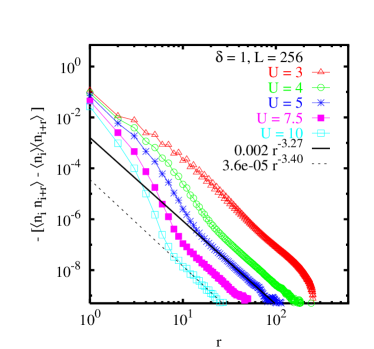
Figure 15: The negative of the density-density correlation function $-\left[\langle n_{i}n_{i+r}\rangle-\langle n_{i}\rangle\langle n_{i+r}\rangle\right]$ for $U>U_{\text{c2}}$. The indicated lines are least-squares fits over a range of $r$ in which the behavior is linear on the log-log scale.

Here we investigate the level crossing point of the ground state and the first excited state $U_{\text{x}}$, as well as the crossing of the first and second excited states $U_{\text{xx}}$. In Ref. Torio, (and further references therein), the crossing points of ground and excited states of finite systems are associated with phase transition points. In particular, the crossing of the ground state and the first excited state with opposite site-inversion parity were shown to correspond to a jump in the charge Berry phase. The crossing of the first and second excited states which are spin singlets and spin triplets with opposite site-inversion symmetry and zero total momentum was argued to be associated with a jump in the spin Berry phase and to characterize a second transition. While the direct calculation of the Berry phases is beyond the scope of this paper, it is possible for us to analyze the finite-size behavior of the level crossings $U_{\text{x}}$ and $U_{\text{xx}}$. We therefore must calculate the energies of the ground state and the first two excited states simultaneously. Sufficiently accurate DMRG results for these energies can only be obtained for system sizes of up to $L=64$, small compared to the ones studied for OBC’s, but nevertheless much larger than the ones that can be reached with exact diagonalization.Torio ; Gidopoulos ; Pati ; Brune We show results for PBC’s for systems with $L=12$, 16, 24, 32, and 64, i.e., system sizes with $4n$ sites, so that the site-inversion symmetry of the ground state is guaranteed to change sign with $U$, as discussed in Sec. I.2. We find non-monotonic behavior of the level crossing points as a function of system size at a scale beyond the system sizes which can be investigated using exact diagonalization.

The finite-size scaling of $U_{\text{x}}$ and $U_{\text{xx}}$ for $\delta=1$ is shown in Fig. 16. The error bars result from the uncertainty in determining the closing or crossing points as well as from the poorer convergence of the DMRG algorithm for PBC’s. Nevertheless, for $\delta=1$ they only are of the order of the symbol size or smaller. For $\delta=4$ and $\delta=20$, the convergence for $L=64$ is poorer around $U_{\text{x}}$ and $U_{\text{xx}}$, but we obtain qualitatively similar behavior up to the larger error bars.

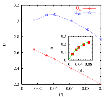
Figure 16: Crossing points of excited states for PBC’s for $\delta=1$ as a function of inverse system size. The inset shows the extrapolation of $\Delta_{\text{S}}(U_{\text{xx}})$ as a function of inverse system size.

For all $\delta$ studied, the finite-size extrapolation of $U_{\text{x}}$ leads to critical couplings in agreement with the ones given in Sec. II.3, up to the smaller numerical accuracy available with PBC’s. Using a quadratic polynomial for the extrapolation, we find $U_{\text{x}}(\delta=1)=2.71$, $U_{\text{x}}(\delta=4)=5.63$ and $U_{\text{x}}(\delta=20)=21.42$. (Due to complicated finite-size effects, we only use the data for $L\leq 32$ for $\delta=4$ and $\delta=20$.) The angle of crossing of $E_{0}$ and $E_{1}$ decreases with increasing system size. This is consistent with a continuous critical behavior at $U_{\text{c1}}$ in the thermodynamic limit.

The non-monotonic behavior of $U_{\text{xx}}$, as seen in Fig. 16, makes an $L\to\infty$ extrapolation difficult. In fact, an extrapolation using the system sizes available to exact diagonalization would give a $U_{\text{c2}}$ which is substantially larger than if the two largest system sizes were included. This could explain the discrepancy in the size of the region between the two critical points found here and obtained in Ref. Torio, . By extrapolating the finite-size data using a quadratic polynomial in $1/L$, we obtain $U_{\text{xx}}(L=\infty,\delta=1)=2.84$, $U_{\text{xx}}(L=\infty,\delta=4)=5.97$, and $U_{\text{xx}}(L=\infty,\delta=20)=21.75$. The values for $U_{\text{xx}}$ and for $U_{\text{c2}}$ obtained from the BO susceptibility are in fairly good agreement. The differences indicate that even larger system sizes are needed to perform an accurate finite-size extrapolation for PBC’s.

Since the transition $U_{\text{c2}}$ is associated with the closing of the spin gap, the gap to the excitations at $U_{\text{xx}}$ should scale to zero with system size. The inset of Fig.  16 shows that $\Delta_{\text{E}}(U_{\text{xx}})=\Delta_{\text{SE}}(U_{\text{xx}})$ indeed closes in the thermodynamic limit. Since one of the two states that are degenerate at $U_{\text{xx}}$ is a spin triplet, this implies a vanishing spin gap. We thus obtain further (indirect) evidence that the couplings at which the BO susceptibility diverges and the spin gap closes coincide, consistent with a two-critical-point scenario. In particular, the angle of the crossing of the first and second excited state also decreases with increasing $L$, consistent with a continuous transition at $U_{\text{c2}}$.

VI Summary

In this paper, we have presented density-matrix renormalization group results that elucidate the nature of the quantum critical behavior found in the half-filled ionic Hubbard model. By carrying out extensive and precise numerical calculations and by carefully choosing the quantities used to probe the behavior, we have been able to investigate the structure of the transition more accurately than in previous work. This has allowed us to resolve a number of outstanding uncertainties and ambiguities. We have worked at three different strengths of the alternating potential $\delta$ covering a significant part of the parameter space and find the same qualitative behavior for all three $\delta$-values. In particular, we have carried out extensive finite-size scaling analyses of three different kinds of gaps: the exciton gap, the spin gap, and the one-particle gap. We find that for fixed $\delta$ and in the thermodynamic limit, the exciton gap goes to zero as a function of $U$ at a first critical point $U_{\text{c1}}$, the spin gap goes to zero at a distinct second critical point $U_{\text{c2}}>U_{\text{c1}}$ and is clearly nonzero at $U_{\text{c1}}$. The one-particle gap (the two-particle gap behaves similarly) reaches a minimum close to $U_{\text{c1}}$, but never goes to zero and never becomes smaller than the spin gap.

Due to the explicitly broken one-site translational symmetry, the ionicity is finite for all finite $U$. For $U\gg\delta$ the ionicity found numerically agrees very well with the one obtained analytically from the strong coupling mapping of the ionic Hubbard model onto an effective Heisenberg model.

We have also studied the bond-order parameter, the order parameter associated with dimerization, as well as the associated bond-order susceptibility. The result of the delicate finite-size extrapolation indicates that there is a finite bond-order parameter in the intermediate region between $U_{\text{c1}}$ and $U_{\text{c2}}$. There is a divergence in the bond-order susceptibility at both $U_{\text{c1}}$ and at $U_{\text{c2}}$, as one would expect from two continuous quantum phase transitions. However, the bond-order susceptibility diverges in the entire strong coupling phase $U\geq U_{\text{c2}}$, albeit more weakly than at $U_{\text{c1}}$. We have pointed out that this is in accordance with the behavior found in the strong coupling phase of the ordinary Hubbard model.

We find that the electric susceptibility is finite for $U<U_{\text{c1}}$ but diverges roughly as $L^{1.5}$ at $U_{\text{c1}}$. This divergence is weaker than the one found for non-interacting electrons (with $\delta=0$) and in the metallic phase of the $t$-$t^{\prime}$-Hubbard model.Aebischer A finite-size scaling analysis of both the bond-order susceptibility and the electric susceptibility yield the same critical exponents at $U_{\text{c1}}$. However, the value, $\eta_{1}\approx 0.45$, is not consistent with the critical exponents of the classical two-dimensional Ising model.Fabrizio

The electric susceptibility also seems to diverge, albeit quite weakly, for $U\geq U_{\text{c2}}$. Correspondingly, the density-density correlation function has a long-distance decay which is of power-law form, but with a small prefactor which becomes smaller with increasing $U$, and a relatively large exponent of approximately $3-3.5$. We speculate that this behavior is related to mixed spin and charge character of excitations present in the strong coupling phase of the ionic Hubbard model, in contrast to the ordinary Hubbard model.

We point out that the divergence of the electric susceptibility at $U_{\text{c1}}$ and for $U\geq U_{\text{c2}}$ does not necessarily imply a finite Drude weight. Based on our results for various energy gaps and the electric susceptibility, we therefore cannot unambiguously classify all different phases and transition points as being metallic or insulating.

Finally, we have presented DMRG results for the position of the crossing of the ground state and the first excited $U_{\text{x}}$ and the crossing of the first two excited states $U_{\text{xx}}$ on systems with periodic boundary conditions on up to 64 sites. The finite-size extrapolation of $U_{\text{x}}$ gives $U_{\text{c1}}$. Due to the loss of accuracy, it is somewhat less clear that the finite-size extrapolation of $U_{\text{xx}}$ corresponds to $U_{\text{c2}}$.

References

- (1) N. Nagaosa and J. Takimoto, J. Phys. Soc. Jpn. 55 2735 (1986).
- (2) J. Hubbard and J.B. Torrance, Phys. Rev. Lett. 47, 1750 (1981).
- (3) T. Egami, S. Ishihara, and M. Tachiki, Science 261, 1307 (1993); S. Ishihara, T. Egami, and M. Tachiki, Phys. Rev. B 49, 8944 (1994).
- (4) Z.G. Soos and S. Mazumdar, Phys. Rev. B 18, 1991 (1978).
- (5) R. Resta and S. Sorella, Phys. Rev. Lett. 74, 4738 (1995); ibid. 82, 370 (1999).
- (6) P.J. Strebel and Z.G. Soos, J. Chem. Phys. 53, 4077 (1970).
- (7) G. Ortiz, P. Ordejón, R.M. Martin, and G. Chiappe, Phys. Rev. B 54, 13515 (1996).
- (8) M. Fabrizio, A.O. Gogolin, and A.A. Nersesyan, Phys. Rev. Lett. 83, 2014 (1999); Nucl. Phys. B 580, 647 (2000).
- (9) T. Wilkens and R.M. Martin, Phys. Rev. B 63, 235108 (2001).
- (10) M.C. Refolio, J.M. Lòpez Sancho, and J. Rubio, cond-mat/0210462 (unpublished).
- (11) M.E. Torio, A.A. Aligia, and H.A. Ceccatto, Phys. Rev. B 64, 121105 (2001).
- (12) N. Gidopoulos, S. Sorella, and E. Tosatti, Eur. Phys. J. B 14, 217 (2000).
- (13) Y. Anusooya-Pati, Z.G. Soos, and A. Painelli, Phys. Rev. B 63, 205118 (2001).
- (14) P. Brune, G.I. Japaridze, A.P. Kampf, and M. Sekania, cond-mat/0106007 v1 and v2 (unpublished) and cond-mat/0304697 (unpublished).
- (15) Y. Takada and M. Kido, J. Phys. Soc. Jpn. 70 21 (2001).
- (16) S. Qin, J. Lou, T. Xiang, G.-S. Tian, and Z. Su, cond-mat/0004162 v1 and v2 (unpublished).
- (17) Y.Z. Zhang, C.Q. Wu, and H.Q. Lin, Phys. Rev. B 67, 205109 (2003).
- (18) S. Caprara, M. Avignon, and O. Navarro, Phys. Rev. B 61, 15667 (2000).
- (19) S. Gupta, S. Sil, and B. Bhattacharyya, Phys. Rev. B 63, 125113 (2001).
- (20) K. Požgajčić and C. Gros, cond-mat/0301376 (unpublished).
- (21) J. Voit, J. Phys. C: Solid State Phys. 21, L1141 (1988).
- (22) F. Gebhard, The Mott Metal-Insulator Transition (Springer-Verlag, Berlin, 1997).
- (23) J. des Cloizeaux and J.J. Pearson, Phys. Rev. 128, 2131 (1962).
- (24) K. Schönhammer, O. Gunnarsson, and R.M. Noack, Phys. Rev. B 52, 2504 (1995).
- (25) S. Manmana, Diploma thesis, Universität Göttingen (2002).
- (26) S. Sachdev, Quantum Phase Transitions (Cambridge University Press, Cambridge, 1999).
- (27) H. Bethe, Z. Physik 71, 205 (1931); L. Hulthén, Arkiv Mat. Astron. Fysik 26A, 1 (1938).
- (28) Close to a critical point, the linear response regime shrinks and very small amplitudes of the external field are required.
- (29) E. Jeckelmann, Phys. Rev. Lett. 89, 236401 (2002).
- (30) C. Aebischer, D. Baeriswyl, and R.M. Noack, Phys. Rev. Lett. 86, 468 (2001).