Ground-state energy fluctuations in the Sherrington-Kirkpatrick model

Abstract

The probability distribution function (PDF) of the ground-state energy in the Sherrington-Kirkpatrick spin-glass model is numerically determined by collecting a large statistical sample of ground states, computed using a genetic algorithm. It is shown that the standard deviation of the ground-state energy per spin scales with the number of spins, $N$, as $N^{-\rho}$ with $\rho\simeq 0.765$, but the value $\rho=3/4$ is also compatible with the data, while the previously proposed value $\rho=5/6$ is ruled out. The PDF satisfies finite-size scaling with a non-Gaussian asymptotic PDF, which can be fitted remarkably well by the Gumbel distribution for the $m$-th smallest element in a set of random variables, with $m\simeq 6$.

Models with quenched disorder describe a wide class of systems in physics and other fields books ; YOUNG . In thermal systems, the effects of disorder are especially important at low temperatures, where the physics is dominated by the low-energy states. These states are also of direct interest in many applications, for instance to combinatorial search problems books . Understanding the properties of the low-energy states is therefore a central task.

In this context, an important aspect concerns the statistical fluctuations of the energy of the low-lying states with respect to the disorder. Consider a system described by an energy function $H_{N}({\bf S},{\bf J})$, where ${\bf S}$ represents $N$ degrees of freedom and ${\bf J}$ a set of quenched random variables signifying the disorder. The ground-state energy per degree of freedom, $e_{N}\equiv N^{-1}\min_{{\bf S}}H_{N}({\bf S},{\bf J})$, when considered as a function of ${\bf J}$, is also random variable, and typically one would like to know its mean $\langle e_{N}\rangle$, standard deviation $\sigma_{N}=(\langle e_{N}^{2}\rangle-\langle e_{N}\rangle^{2})^{1/2}$, and possibly its entire PDF, $p_{N}(e_{N})$. In the thermodynamic limit, $N\to\infty$, usually the properties of extensivity ($\langle e_{N}\rangle\to e_{0}$, with $e_{0}$ a quantity of order one) and self-averaging ($\sigma_{N}\to 0$) hold, so one simply has $p_{N}(x)\to\delta(x-e_{0})$. Thus, the interesting question is to determine the finite-$N$ scaling behavior. More precisely, one may ask for example:

(i) How does $\langle e_{N}\rangle$ scale with $N$?

(ii) How does $\sigma_{N}$ scale with $N$?

(iii) Given the natural scaling variable $y_{N}=(e_{N}-\langle e_{N}\rangle)/\sigma_{N}$, does its PDF $\tilde{p}_{N}(y_{N})$ converge for large $N$ to a nontrivial asymptotic PDF, $\tilde{p}_{\infty}(y_{N})$?

To leading order, we expect $\langle e_{N}\rangle=e_{0}+bN^{-\omega}$ and $\sigma_{N}\sim N^{-\rho}$, so (i) and (ii) amount to determine the exponents $\omega$ and $\rho$. Question (iii) amounts to determine whether the scaling relation

$$p_{N}(e_{N})={1\over\sigma_{N}}\,\tilde{p}_{\infty}\left(\frac{e_{N}-\langle e_{N}\rangle}{\sigma_{N}}\right)$$ (1)

holds for large $N$, and the shape of $\tilde{p}_{\infty}(x)$. The answer to (ii) and (iii) is simple for systems with short-range interactions, where the volume can be subdivided so that $e_{N}$ is the sum of $O(N)$ nearly independent contributions. For the central limit theorem, then, $\sigma_{N}\sim N^{-1/2}$ (as rigorously proven for short-range spin glasses aw ) and $\tilde{p}_{\infty}(x)$ is a Gaussian for moderate values of $x$ (we will not be concerned with large deviations here). For sufficiently long interaction range, in general one has $\rho\neq 1/2$ and a non-Gaussian $\tilde{p}_{\infty}(x)$ foot_diluted .

In this paper, the questions above are addressed numerically for the infinite-range Sherrington-Kirkpatrick (SK) spin-glass model sk . Much is known about this model, following Parisi’s replica-symmetry-breaking (RSB) solution rsb ; books , but many issues remain open, finite-size scaling being a prominent one. The exponents $\omega$ and $\rho$ remain unknown analytically, while previous numerical work indicates $\omega\simeq 2/3$ thesis ; krzakala ; boettcher an $\rho\simeq 3/4$ cabasino ; krzakala . Determining the full ground-state energy PDF is a much more challenging task, which so far has received limited attention krzakala . Here, we will address these issues with a much higher statistics than in previous studies.

The interest of this problem lies also in its relationship bouchaud with extreme value statistics gumbel . The goal of extreme value statistics is to determine whether the PDF of the $m$-th smallest value $X$ in a set of random variables $X_{1},\dots,X_{M}$ (the energy levels in our case) approaches a scaling form $p_{M}(X)=1/b_{M}\,\tilde{p}_{\infty}[(X-a_{M})/b_{M}]$ for large $M$, with suitable $a_{M},b_{M}$. The case of independent, identically distributed (i.i.d.) $X_{i}$’s is well understood gumbel : if scaling holds, $\tilde{p}_{\infty}(x)$ is one of three universal distributions, depending on the PDF of the $X_{i}$’s. If the latter is unbounded and decays faster than a power law for large $|X_{i}|$, then $\tilde{p}_{\infty}(x)$ is the Gumbel PDF (defined below). An example of a disordered system with i.i.d. energy levels is the Random Energy Model rem , but in general the levels are correlated, and this case is much less understood (an exception is when $e_{N}$ is the sum of spatially uncorrelated variables, as mentioned above). The Gumbel form is preserved for short-range correlations and violated for sufficiently long-range correlations gumbel ; bouchaud . It is therefore interesting to ask if it applies, at least approximately, to the SK model, where full RSB leads to hierarchically correlated energy levels (see, however, Ref. dean, for a model with hierarchical correlations giving a non-universal PDF).

Numerical details – We study the standard SK model with energy function

$$H_{N}=-\sum_{i<j}J_{ij}S_{i}S_{j}$$ (2)

where the $S_{i}$’s are $N$ Ising spins ($S_{i}=\pm 1$) and the $J_{ij}$’s are i.i.d. random variables drawn from a Gaussian PDF with zero mean and variance $1/N$. The sizes studied are $N=19,39,59,99$, and $199$ with, respectively, 250000, 250000, 180000, 120000, and 64000 independent realizations of the disorder (samples). The ground state of each sample was determined using a genetic algorithm pal ; py . The $l$-th order cumulants of $p_{N}(e_{N})$, denoted by $k_{l,N}$, and their statistical errors were then estimated with a bootstrap method foot_jack up to $l=5$. With large statistics, it is especially important to control the systematic errors due to occasionally missing the ground state. This was done by performing much longer runs for a fraction of the samples, checking that the change in the cumulants was smaller than the desired statistical error.

Scaling of the mean and standard deviation – Previous numerical studies indicate a value $\omega\simeq 2/3$ for both the SK model thesis ; krzakala and diluted spin glasses thesis ; krzakala ; boettcher ; liers . The analytical result $\omega=2/3$ was obtained for the finite-size scaling of the internal energy near $T_{c}$ and the Almeida-Thouless line slanina , but no result is available deep in the ordered phase. Our data for $\langle e_{N}-e_{0}\rangle N^{2/3}$, using the exact Parisi result rsb $e_{0}=-0.7633\dots$, are shown in the inset of Fig. 1. The small residual dependence on $N$ foot_error either indicates that $\omega$ is greater than 2/3 or, if $\omega=2/3$, that the data are accurate enough to resolve subleading corrections. A fit with $\langle e_{N}\rangle=-0.7633+bN^{-\omega}$ gives $\omega=0.673\pm 0.002$ ($\chi^{2}=11.2$, ${\mbox{ndf}}=3$, ndf being the number of degrees of freedom), where the error gives the range for which the goodness-of-fit $Q$ is larger than $10^{-3}$. A fit with $\omega=2/3$ (leaving $b$ as the only free parameter) gives $Q<10^{-16}$, which is clearly not acceptable. Nevertheless, since corrections of just a few percent could accommodate the value $\omega=2/3$ (note the vertical scale in the inset of Fig. 1), this value cannot be ruled out. Fits with corrections (for example $\langle e_{N}-e_{0}\rangle N^{\omega}=b+cN^{-\omega_{2}}$ with fixed $e_{0}$ and $\omega$) are not conclusive since the corrections are small and thus the parameter range is large.

Turning now to the fluctuations, in the replica formalism one can write the cumulant generating function of the (quenched) free-energy as the annealed free energy of $n$ replicas, $f(n)$. Crisanti et al. crisanti argued that if the first nonlinear term in the small-$n$ expansion of $f(n)$ is $n^{i}$ (in the thermodynamic limit) then $\rho=1-1/i$. Kondor kondor found $f(n)=nf-cn^{6}$ from the “truncated model”, which would imply $\rho=5/6$. Recently, Aspelmeier and Moore aspel and De Dominicis and Di Francesco dedominicis found a higher free-energy (hence better) solution $f(n)=nf$, from which the conclusion $\rho=5/6$ no longer follows, and Refs. aspel2, ; krzakala, gave qualitative arguments indicating $\rho=3/4$. On the numerical side, Cabasino et al. cabasino found a result compatible with $\rho=3/4$, but with large statistical errors, and Bouchaud et al. krzakala found $\rho\simeq 0.76$, also compatible with $3/4$, but they could not rule out $\rho=5/6$.

Figure 1: Standard deviation of the ground-state energy per spin as a function of the system size. The lines represent the power-law $\sigma_{N}=aN^{-\rho}$ for three values of $\rho$. Inset: finite-size deviation of the mean from the RSB result rsb $e_{0}=-0.7633$.

Our numerical data for $\sigma_{N}$ are displayed in Fig. 1, multiplied by $N^{1/2}$ to stress that $\sigma_{N}$ decays faster with $N$ than in short-range models. An exponent $\rho=3/4$ follows reasonably well the data, but deviations can be noticed. These are seen more clearly in the plot of $N^{3/4}\sigma_{N}$ in Fig. 2(a). Here the curvature in the data demonstrates the presence of subleading corrections. The dashed line represents a power law fit $\sigma_{N}=aN^{-\rho}$ for $N\geq 59$, which gives $\rho=0.765\pm 0.01$ ($\chi^{2}=3.93,{\mbox{ndf}}=1$), in agreement with $\rho=3/4$ (the error corresponds again to $Q>10^{-3}$). However, the decreasing trend for large $N$ foot_error and the negative curvature suggest that $\rho$ may in fact be greater than $3/4$. As for the mean, fits with correction terms (for fixed $\rho$) are not very illuminating. Fig. 1 also shows that $\rho=5/6$ clearly does not fit the data, as seen also in Fig. 2(b) where $N^{5/6}\sigma_{N}$ is far from constant. Since the sizes considered are already well in the scaling regime (at least as far as Eq.(1) is concerned, see below), crossover to a constant for larger $N$ is rather unlikely, hence we conclude that $\rho=5/6$ is ruled out. Finally, if $\sigma_{N}\sim N^{-\rho}$ and Eq.(1) holds, then $k_{l,N}\sim N^{-l\rho}$. Figs. 2(c) and 2(d) show that also for $l=3,4$ the data agree with $\rho\simeq 3/4$ but not with $\rho=5/6$ (note that the statistical error is much larger than that of $\sigma_{N}$).

Figure 2: Plots of $\sigma_{N}N^{\rho}$ for $\rho=3/4$ (a) and $\rho=5/6$ (b), and of $k_{l,N}N^{l\rho}$ for $\rho=3/4$, $l=3$ (c) and $\rho=3/4$, $l=4$ (d). The dashed line in (a) is the best fit $\sigma_{N}=aN^{-\rho}$ for $N\geq 59$, giving $\rho=0.765$. The dotted lines in (c) and (d) represent power laws $N^{-l\rho}$ with $\rho=5/6$.

Scaling of the PDF – Scaling plots of $p_{N}(e_{N})$ according to Eq.(1) are shown in Fig. 3 and, on a logarithmic scale, Fig. 4. The data collapse is remarkably good, indicating that we are already well in the scaling regime. Comparison with a Gaussian PDF, represented by the dashed lines in Figs. 3 and 4, clearly indicates a non-Gaussian behavior. Table I displays the scaled cumulants $\tilde{k}_{l,N}\equiv k_{l,N}/\sigma_{N}$ for $l=3,4,5$ (since $\tilde{k}_{2,N}=1$ by definition, $\tilde{k}_{3,N}$ is the skewness and $\tilde{k}_{4,N}$ the kurtosis of $\tilde{p}_{N}$): the cumulants are independent of $N$ within the errors, again strongly supporting scaling (small deviations exist for $N=19$ and $l=3,4$, presumably due to corrections to scaling). Note that scaling of the PDF is independent of the values of $\omega$ and $\rho$.

Next, we compare the scaled PDF to known theoretical distributions. The Gumbel PDF for the $m$-th smallest in a set of i.i.d. random variables has the form gumbel ; foot_gumbel

$$g_{m}(x)=w\exp\left[m{x-u\over v}-m\exp{x-u\over v}\right]$$ (3)

where $u$ and $v$ are rescaling parameters and $w$ a normalization constant. To compare this to our data, we impose zero mean and unit variance which, together with normalization, fixes $u$, $v$, and $w$ as a function of $m$. Expressions for the cumulants of $g_{m}(x)$ are easily obtained. These are decreasing functions of $m$, in absolute value, and vanish for large $m$, thus $g_{m}$ provides an interpolation between the standard Gumbel ($m=1$) and a Gaussian PDF ($m=\infty$). As shown in Table I, the cumulants are fitted well for $m=6\pm 0.3$ ($\tilde{k}_{5,N}$ shows small deviations from the $N\leq 39$ data, possibly an effect of corrections to scaling). Table I also shows that $m=\pi/2$ (see below) is far from agreeing with the data, hence even more so is $m=1$, as also noted in Ref. krzakala, . This shows that the correlations in the energy levels give rise to a more Gaussian-like PDF with respect to the uncorrelated ($m=1$) case. The PDF $g_{6}(x)$ is displayed with solid lines in Figs. 3 and 4, and the corresponding cumulative distribution in the inset of Fig. 3: the agreement with the data is excellent everywhere. Although it is not clear why a Gumbel distribution with $m\neq 1$ should work here, $g_{6}(x)$ can certainly be used to accurately represent the true PDF up to several standard deviations. It would be interesting to reach higher statistics to check whether the agreement breaks down. Incidentally, the Gumbel distribution with a non-integer value $m=\pi/2$ has been conjectured to describe bramwell , at least to a good approximation, the PDF of spatially averaged quantities in many correlated systems, even when no extreme value is apparently involved. A modified Gumbel form with non-integer $m$ was also used to describe the order-parameter PDF in three-dimensional spin glasses berg .

Another example of extreme value of correlated random variables is the smallest eigenvalue, $\lambda_{M}$, of an $M\times M$ random matrix. For three well-known ensembles, the scaling PDF of $\lambda_{M}$ is the Tracy-Widom (TW) distribution tw , $f_{\beta}(x)$, with $\beta$ a parameter dependent on the ensemble. We tested it against our data finding a poor agreement, although better than for $g_{1}(x)$. Table I shows that the cumulants for $\beta=1$ (and thus for $\beta=2$), computed from the tabulated $f_{\beta}(x)$ spohn , are well outside the statistical errors. The PDF $f_{1}(x)$ is displayed with dotted lines in Figs. 3 and 4: one can see small deviations from the data for small $x$ and large deviations in the tails.

In conclusion, we presented accurate numerical data consistent with $\omega=2/3$ and $\rho=3/4$ when considering subleading corrections, although both exponents may be in fact slightly larger than these values. The PDF of the ground-state energy satisfies finite-size scaling with an asymptotic PDF empirically well described by a Gumbel distribution.

After this work was virtually finished, we learned that $p_{N}(e_{N})$ was also studied numerically in Ref. andreanov, .

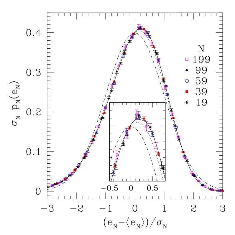
Figure 3: Scaling plot of the ground-state energy PDF. The solid line is the Gumbel PDF with $m=6$ ($u=0.2011219,v=2.348408,w=165.5589$). The dotted line is the Tracy-Widom PDF with $\beta=1$. The dashed line is a Gaussian PDF. All PDF’s are normalized to one and have zero mean and unit variance. The inset shows a zoom near the origin.

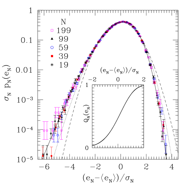
Figure 4: Same as Fig. 3 but on a semi-logarithmic scale. Inset: scaling plot of the cumulative distribution $Q_{N}(e_{N})=\int_{-\infty}^{e_{N}}p_{N}(x)\,dx$ for $N=19,39,59,99,199$, and of the Gumbel cumulative distribution for $m=6$. The curves all fall on top of each other within the line thickness.

N	$-\tilde{k}_{3,N}$	$\tilde{k}_{4,N}$	$-\tilde{k}_{5,N}$
19	$0.467\pm 0.007$	$0.42\pm 0.02$	$0.46\pm 0.07$
39	$0.422\pm 0.007$	$0.35\pm 0.02$	$0.31\pm 0.05$
59	$0.413\pm 0.008$	$0.35\pm 0.02$	$0.32\pm 0.07$
99	$0.420\pm 0.010$	$0.37\pm 0.03$	$0.40\pm 0.08$
199	$0.409\pm 0.015$	$0.41\pm 0.04$	$0.68\pm 0.15$
$g_{6}$	0.42468	0.35346	0.4441
$g_{\pi/2}$	0.89373	1.53674	3.8403
$f_{1}$	0.2935	0.16524	0.1024
$f_{2}$	0.2241	0.09345	0.0386

Table 1: Cumulants of the scaled PDF $\tilde{p}_{N}(y_{N})$ for various values of $N$, compared with the cumulants of the theoretical PDF’s $g_{m}(x)$ (Gumbel distribution for $m$-th largest extreme) and $f_{\beta}(x)$ (Tracy-Widom distribution).

Acknowledgements – The author thanks A.P. Young and M.A. Moore for very useful exchanges, and the authors of Ref. andreanov, for communicating some of their findings prior to publication. The author also thanks M. Mézard for a useful discussion and M. Prähofer and H. Spohn for making their computation of the TW distribution publicly available spohn . Support from STIPCO, EC grant number HPRN-CT-2002-00319, is acknowledged.

References

- (1)
- (2) M. Mézard, G. Parisi, and M.A. Virasoro, Spin Glass Theory and Beyond (World Scientific, Singapore, 1987).
- (3) Spin Glasses and Random Fields, A.P. Young Ed. (World Scientific, Singapore, 1998).
- (4) J. Wehr and M. Aizenmann, J. Stat. Phys. 60, 287 (1990).
- (5) Interestingly, infinite-range spin glasses on finite-connectivity graphs seem to behave like the short-range case krzakala , although the same argument cannot be applied.
- (6) D. Sherrington and S. Kirkpatrick, Phys. Rev. Lett. 35, 1792 (1975).
- (7) G. Parisi, Phys. Rev. Lett. 43, 1754 (1979); 50, 1946 (1983).
- (8) M. Palassini, PhD thesis, 2000.
- (9) J.-P. Bouchaud, F. Krzakala, and O.C. Martin, cond-mat/0212070.
- (10) S. Boettcher, Eur. Phys. J. B 31, 29 (2003).
- (11) S. Cabasino, E. Marinari, P. Paolucci, and G. Parisi, J. Phys. A 21, 4201 (1988).
- (12) J.-P. Bouchaud and M. Mézard, J. Phys. A 30, 7997 (1997).
- (13) E.J. Gumbel, Statistics of Extremes (Columbia University Press, New York, 1958); J. Galambos, The Asymptotic Theory of Extreme Order Statistics (R.E. Krieger Publishing Co., Malabar, FL, 1987).
- (14) B. Derrida, Phys. Rev. B 24, 2613 (1981); D.J. Gross and M. Mézard, Nucl. Phys. B 240, 431 (1984).
- (15) D.S. Dean and S.N. Majumdar, Phys. Rev. E. 64, 046121 (2001).
- (16) K. F. Pal, Physica A 223, 283 (1996).
- (17) M. Palassini and A.P. Young, Phys. Rev. Lett. 83, 5126 (1999).
- (18) A jackknife method was also tried, but this performed poorly for large-order cumulants.
- (19) F. Liers, M. Palassini, A.K. Hartmann, and M. Juenger, cond-mat/0212630.
- (20) G. Parisi, F. Ritort, and F. Slanina, J. Phys. A 26, 247 (1993); J. Phys. A 26, 3775 (1993).
- (21) The decreasing trend for large in the inset of Fig. 1 and in Fig. 2(a) is not due to systematic errors from occasionally missing the ground state at large , since these would give higher values of both and (this was also verified numerically by performing shorter runs).
- (22) A. Crisanti, G. Paladin, H.-J. Sommers, and A. Vulpiani, J. Phys. I France 2, 1325 (1992).
- (23) I. Kondor, J. Phys. A 16, L127 (1983).
- (24) T. Aspelmeier and M.A. Moore, Phys. Rev. Lett. 90, 177201 (2003).
- (25) C. De Dominicis and P. Di Francesco, cond-mat/0301066.
- (26) T. Aspelmeier, M.A. Moore, and A.P. Young, Phys. Rev. Lett. 90, 127202 (2003).
- (27) The case is properly known as the Gumbel distribution, while the more general case is often called Fisher-Tippett distribution.
- (28) S.T. Bramwell et al., Phys. Rev. Lett. 84, 3744 (2000); Phys. Rev. E 63, 041106 (2001).
- (29) B.A. Berg, A. Billoire, and W. Janke, Phys. Rev. E 65, 045102R (2002).
- (30) C.A. Tracy and H. Widom, Comm. Math. Phys. 159, 151 (1994); 177, 727 (1996).
- (31) M. Prähofer and H. Spohn, Physica A 279, 342 (2000); Phys. Rev. Lett. 84, 4882 (2000); J. Stat. Phys. 108, 1071 (2002); Data available at http://www-m5.mathematik.tu-muenchen.de/KPZ/.
- (32) A. Andreanov, F. Barbieri, and O.C. Martin, cond-mat/0307709.