Large deviations in spin-glass ground-state energies

Abstract

The ground-state energy $E_{0}$ of a spin glass is an example of an extreme statistic. We consider the large deviations of this energy for a variety of models when the number of spins $N$ goes to infinity. In most cases, the behavior can be understood qualitatively, in particular with the help of semi-analytical results for hierarchical lattices. Particular attention is paid to the Sherrington-Kirkpatrick model; after comparing to the Tracy-Widom distribution which follows from the spherical approximation, we find that the large deviations give rise to non-trivial scaling laws with $N$.

1 Introduction

Systems with quenched disorder have been studied intensively for the last two decades. Thermodynamic properties such as the free energy in these systems fluctuate from sample to sample, but not very much: indeed, they are self-averaging if the disorder does not have long range correlations LifshitzGredeskul88 . This means that typical values of the free energy density (to name but one quantity) deviate arbitrarily little from a fixed value in the large volume limit. Because of this, little work has considered large deviations, i.e., the probability of finding a rare sample (realization of the disorder) for which the free energy density deviates from the typical value by a significant amount.

In spin glasses, the archetype of disordered systems with frustration, the large deviations of thermodynamic quantities have been studied so far in only 3 very special cases: (1) the Random Energy Model Derrida80 (REM) which can be treated completely because of its extreme simplicity; (2) the Generalized REM Derrida85 for which bounds have been obtained BovierKurkova03 on the probability of large deviations; (3) the Sherrington-Kirkpatrick model SherringtonKirkpatrick75 but with results Talagrand00 in the paramagnetic phase only. This last model is important because, in contrast to the first two cases, it is based on a microscopic Hamiltonian with spins, a necessary step to have a realistic model. In the study that follows, we work well in the spin-glass phase for a variety of realistic models, focusing on the statistics of the system’s ground-state energy $E_{0}$. In particular, we consider a nearly soluble case associated with hierarchical lattices that gives some qualitative insights into the properties of the large deviations function.

The outline of this paper is as follows. We first introduce some definitions and notation in Section 2, recalling some general results on large deviations. In the rest of the paper, we tackle successively different models of spin glasses. Section 3 covers a class of hierarchical models for which both analytic and numerics can be pushed very far. Section 4 deals with the REM which is exactly solvable. These two models of spin glasses display the importance of summing/minimizing over random variables. In Section 5 the properties of $E_{0}$ in the Sherrington-Kirkpatrick model are examined numerically; first its distribution is compared to the Tracy-Widom one, and then we investigate the scaling variables entering into different large deviations functions. In Section 6 we consider both Edwards-Anderson and mean field models of spin glasses for which the connectivity is finite. Our numerical analysis shows that their properties are close to those found in the hierarchical lattices. Overall conclusions are given in Section 7.

2 General results on large deviations

Consider a physical observable $z_{N}$ of a system of $N$ spins in the presence of quenched disorder; in our study $z_{N}$ will be the ground-state energy density, $E_{0}/N$. Usually, $z_{N}$ satisfies two convergence properties. First, the distribution of $z_{N}$ becomes peaked around $z^{*}$ at large $N$:

$$\forall\varepsilon>0,\quad P\{|z_{N}-z^{*}|\geq\varepsilon\}\to 0\quad\mbox{as }\ N\to\infty\ .$$ (1)

A familiar context where this arises is when averaging a large number of independent identically distributed (i.i.d. hereafter) random variables: the weak law of large numbers says that such an average becomes peaked Feller50 when $N\to\infty$. Second, the sequence $\{z_{N}\}$ itself converges “almost always”: if one successively adds spins, thereby increasing $N$ and adding the corresponding coupling terms to the Hamiltonian, typical sequences will converge to $z^{*}$. In the context of averages of i.i.d. random variables, this is called the strong law of large numbers. (Note that within Eq. 1, the sequence $\{z_{N}\}$ can deviate arbitrarily from $z^{*}$ as long as such deviations arise more and more rarely as $N\to\infty$.) In physics, the terminology “self-averaging” usually refers to the weak convergence: if $p_{N}$ is the probability density of $z_{N}$, then $p_{N}$ converges to the Dirac distribution $\delta(z_{N}-z^{*})$. It is of interest to understand the nature of this convergence for physical observables; often, it turns out to be “exponential”. More precisely, one says that the distribution of $z_{N}$ satisfies the Large Deviations Principle (LDP in what follows) if for all $t$ one has the following large $N$ asymptotics:

$$p_{N}(z_{N}=t)\sim K(t,N)\ e^{-Nf(t)}$$ (2)

where $K$ is a slowly varying function compared to the exponential. The function $f$ is called the Large Deviations Function (LDF hereafter). In our numerical study, we consider

$$f_{N}(t)=-\frac{1}{N}\ln\left[p_{N}(z_{N}=t)\right]$$ (3)

and then we estimate $f$ via $f_{N}\to f$ as $N\to\infty$. More traditionally, the LDF is defined Bucklew90 from the distribution function of $z_{N}$ which is generally a better quantity to consider mathematically. Introduce the two probabilities $P\{z_{N}\geq t\}$ for $t>z^{*}$ and $P\{z_{N}\leq t\}$ for $t<z^{*}$; from these one defines the LDF $f$ from the limits (if they exist):

$$f(t)=\lim\limits_{N\to\infty}-\frac{1}{N}\ln P\{z_{N}\geq t\}\quad t>z^{*}$$

$$f(t)=\lim\limits_{N\to\infty}-\frac{1}{N}\ln P\{z_{N}\leq t\}\quad t<z^{*}\ .$$ (4)

In the next paragraphs we consider simple examples of the LDP.

2.1 Sums of independent variables

Consider first the case of averages of i.i.d. random variables. Let $\{x_{i}\}$ be i.i.d. variables of probability density $\mu$, and

$$z_{N}=\frac{1}{N}\sum_{i=1}^{N}x_{i}\ .$$ (5)

For any $\lambda$, define

$${\cal L}(\lambda)=\ln\int\mu(x)e^{\lambda x}dx$$ (6)

and

$$f(t)=\max\limits_{\lambda}(\lambda t-{\cal L}(\lambda))\ .$$ (7)

Cramer’s theorem (see for instance ref. Bucklew90 ) states that for any closed set $F$ and any open set $G$

$$\varlimsup_{N\to\infty}\frac{1}{N}\ln P\{z_{N}\in F\}\leq-\inf\limits_{t\in F}f(t)$$

$$\varliminf_{N\to\infty}\frac{1}{N}\ln P\{z_{N}\in G\}\geq-\inf\limits_{t\in G}f(t)$$ (8)

where $\varliminf$ and $\varlimsup$ are the inf and sup limits.

Still sharper asymptotics are provided by the Bahadur-Rao theorem if the first two moments of the $x_{i}$ are finite. Without loss of generality, assume that the $x_{i}$ have a zero mean and a unit variance. Let $\lambda(t)$ be the value of $\lambda$ such that the sup in Cramer’s theorem is reached, i.e., $f(t)=\lambda t-{\cal L}(\lambda)$. Then for all $t>0$, we have

$$\lim\limits_{N\to\infty}P\{z_{N}\geq t\}N^{1/2}e^{Nf(t)}={\left(\lambda(t)\sqrt{2\pi{\cal L}^{{}^{\prime\prime}}\left[\lambda(t)\right]}\right)}^{-1}$$ (9)

as well as the analogous relation for $t<0$.

Let us now apply this framework to one-dimensional spin glasses. Suppose one has a chain of $N$ Ising spins ($S_{i}=\pm 1$) with free boundary conditions described by the Hamiltonian

$$H(\{S_{i}\})=-\sum_{i=1}^{N-1}J_{i,i+1}S_{i}S_{i+1}$$ (10)

where the $J_{i,i+1}$ are i.i.d. random variables with probability density $\rho$. It is easy to see that the ground-state energy density is

$$e_{0}=-\frac{\sum\limits_{i=1}^{N-1}|J_{i,i+1}|}{N}$$ (11)

leading one to the identification $x_{i}=|J_{i,i+1}|$ and then $e_{0}=(1-1/N)z_{N-1}$. The direct application of Cramer’s theorem gives the LDF of the ground-state energy density:

$$f(t)=\max\limits_{\lambda}\left[\lambda t-\ln\int\rho(J)~{}e^{-\lambda|J|}dJ\right]\ .$$ (12)

This last result shows explicitly the non-universality of the large deviations function. To illustrate this, we can compute $f$ for several specific cases. Consider first the discrete distribution

$$\rho(J)=\frac{\delta(J)}{2}+\frac{\delta(|J|-1)}{4}\ .$$ (13)

This model’s ground-state energy density is always negative and its mean is $-1/2$. A simple computation shows that when $t<0$ one has $\exp(\lambda)=(1+t)/(-t)$ while $\lambda=\infty$ for $t\geq 0$. This leads to

$$f(t)=\ln 2+|t|\ln|t|+(1+t)\ln(1+t)$$ (14)

for $-1\leq t\leq 0$ and $f(t)=\infty$ otherwise. Note that $f$ is symmetric about $-1/2$ and that $f(-1/2)=0$ as it should. It is easy to see that any discrete $J$ distribution leads to a bounded range of possible values of $e_{0}$; clearly one has $f(t)=\infty$ outside of this range, but interestingly $f(t)$ is finite at the boundary values. Finally, for the case considered in Eq. 13, we have $f(0)=f(-1)=\ln 2$ but the slope of $f$ is infinite at those points.

Consider now an exponential distribution:

$$\rho(J)=\frac{\alpha e^{-\alpha|J|}}{2}\ .$$ (15)

The mean (typical) value of $e_{0}$ is $-1/\alpha$, and again $e_{0}\leq 0$ but now all negative values of $e_{0}$ can arise. A simple calculation leads to

$$f(t)=-\alpha t-1-\ln(\alpha|t|)\ \mbox{ for }\ t<0$$ (16)

and $f(t)=\infty$ for $t\geq 0$. We now have a logarithmic divergence as $t\to 0^{-}$ while the behavior when $t\to-\infty$ follows that of $-\ln\rho(-|J|=t)$, i.e., $f(t)\sim-\alpha t$. This is a general feature: when $t\to-\infty$ in any spin-glass model, we must have that all the $J$s become large; furthermore there is no more frustration, that is we reach the ferromagnetic limit. Let’s consider this explicitly in the case where $\rho(J)$ is a Gaussian of zero mean and unit variance. A simple computation shows that $f(t)\approx t^{2}/2-\ln 2$ at large negative $t$ which has the same divergence as $-\ln\rho(-|J|=t)$; this pattern will hold in all spin-glass models. The general picture is then that $f(t)=\infty$ for $t>0$ while the $t\to-\infty$ limit simply reflects the asymptotics of $\rho(J)$. This last property shows explicitly why large deviations in spin glasses are not universal. Note that this is in sharp contrast to what happens for the limiting shape of the distribution of $E_{0}$! In the case we are considering, $E_{0}$ is the sum of independent variables; the central limit theorem then shows that the distribution’s shape becomes Gaussian at large $N$.

2.2 Minimum of independent variables

Another quantity of interest in spin glasses is the domain wall energy $\Delta$. This energy is simply the change in the ground-state energy when applying anti-periodic rather than periodic boundary conditions. Using the notation of the previous paragraphs, it is clear that for a chain of $N$ spins

$${\Delta}_{N}={\rm sign}(\prod_{i}J_{i,i+1})\,\min_{i}\{|J_{i,i+1}|\}\ .$$ (17)

The distribution of $\Delta$ is easily obtained in terms of $\rho$, especially if $\rho(J)$ is even in $J$. Limiting ourselves to that case, introduce an integrated distribution function $q_{N}(t)$ of ${|\Delta}_{N}|$:

$$q_{N}(t)\equiv 2\int_{|t|}^{\infty}p_{N}(\Delta_{N})d\Delta_{N}=q_{1}^{N-1}(t)\quad\mbox{for}\quad t\geq 0\ .$$ (18)

The LDF $f(t)$ is of course even and can be obtained directly from Eqs. 2 or 3, leading to

$$f(t)=\ln\left[2\int_{|t|}^{\infty}\rho(J)dJ\right]\ .$$ (19)

Here again one sees that the LDF is sensitive to $\rho(J)$ and thus is not universal. When we consider instead the large $N$ shape of the distribution of $|\Delta_{N}|$, we see that it follows a Weibull Gumbel58 distribution if $\rho(J)$ is smooth; such a limit law is universal…

2.3 Case of general spin-glass models

For an arbitrary Ising spin glass, the Hamiltonian is

$$H(\{S_{i}\})=-\sum_{i<j}J_{ij}S_{i}S_{j}$$ (20)

where the $J_{ij}$ are i.i.d. random variables. The ground-state energy $E_{0}$ is the minimum value of $H$ when considering all the $2^{N}$ assignments of the spin values; the main difference with the domain wall energy case just treated is that these $2^{N}$ random values are correlated. It has been proven for at least some classes of spin glasses LifshitzGredeskul88 that $E_{0}/N$ converges in probability when $N\to\infty$ ($E_{0}$ is self-averaging). Our interest in this work is to find out empirically whether this convergence is exponential or not, i.e., whether there is a LDP. It is difficult to motivate a LDP from the point of view of minimization over $2^{N}$ highly correlated assignments; instead it is better to formulate the problem differently as follows. Rewrite Eq. 20 as a sum of $N$ terms:

$$H(\{S_{i}\})=\sum_{i}\frac{(-\sum_{j\neq i}J_{ij}S_{j})}{2}S_{j}\ .$$ (21)

The ground-state energy $E_{0}$ is then the sum of these $N$ terms when the $S_{i}$ are set to their ground-state values. These different terms are correlated as is clear from the fact that a given $S_{i}$ appears in several such terms, and in contrast to the one dimensional chain, there is no way to change variables so that the terms become independent. Nevertheless, correlations are relatively weak if $H$ is local (that is if the interactions are short range), and probably weak correlations do not spoil the existence of a LDP. In fact, clues to this effect come from extensions of Cramér’s theorem, leading us to try to test for the presence of a LDP in our systems. We now do this in a “hands-on” fashion, using numerical analysis on different spin-glasses models.

3 Migdal-Kadanoff lattices

We begin with the family of models following from the Migdal-Kadanoff (MK) approach SouthernYoung77 ; BerkerOstlund79 where one performs a bond-moving real-space renormalisation group. This procedure effectively amounts to computing quantities on hierarchical (MK) lattices defined recursively. The recursion takes one bond (that is an edge of the current graph) into $b$ paths, each made of $l$ segments. The first iteration is represented in Fig. 1 for $b=4$, $l=2$. In what follows we restrict ourselves to the case $l=2$.

Figure 1: Construction of a Migdal-Kadanoff lattice having $b=4$ branches and $l=2$ segments.

Given such a “lattice”, Ising spins are placed on its sites. The system’s Hamiltonian is then

$$H_{J}=-\sum_{\langle ij\rangle}J_{ij}S_{i}S_{j}$$ (22)

where $S_{i}=\pm 1$ and $\langle ij\rangle$ restricts the sum to nearest neighbors. The $J_{ij}$ are quenched i.i.d. random variables assigned to the edges. In general, they are either Gaussian or bimodal ($J_{ij}=\pm 1$).

Compared to the systems we will consider further on, MK lattices have the advantage of allowing an exact recursion for the ground-state energy. Thus both analytic and numerical computations of the LDF can be performed without too much difficulty, even though $E_{0}$ remains a sum of dependent random variables.

3.1 Definitions

If $g$ is the recursion level (beginning with $g=0$ as shown in Fig. 1), then the “linear” lattice size (or diameter) $L_{g}$ is $2^{g}$ and the volume $N_{g}$ (actually the number of edges or terms contributing to the energy) is ${(2b)}^{g}$. The space dimension $d$ is obtained via the identity $N_{g}=L_{g}^{d}$ so one has $d=1+\ln b/\ln 2$. The usual choice for $d=3$ is $b=4,l=2$, while $b=l=2$ gives $d=2$.

In the recursion relation for the ground-state energy, one needs to keep track of two energies: $E^{(p)}_{g}$ and $E^{(a)}_{g}$. These give the MK lattice ground-state energy at the $g$th generation when the two exterior spins are respectively parallel and antiparallel. The ground-state energy $E_{0}$ then reads:

$$E_{0}=\min\{E^{(p)},E^{(a)}\}\ .$$ (23)

The recursion for a $b$-branch MK lattice with $l=2$ at the $(g+1)$th stage is:

$$\begin{split}E^{(p)}_{g+1}=\sum\limits_{k=1}^{b}\min\{&E^{(p)}_{g}(1,k)+E^{(p)}_{g}(2,k),\\ &E^{(a)}_{g}(1,k)+E^{(a)}_{g}(2,k)\}\end{split}$$ (24)

$$\begin{split}E^{(a)}_{g+1}=\sum\limits_{k=1}^{b}\min\{&E^{(a)}_{g}(1,k)+E^{(p)}_{g}(2,k),\\ &E^{(p)}_{g}(1,k)+E^{(a)}_{g}(2,k)\}\end{split}$$ (25)

where the index $1,2$ refers to the two bonds forming the $k$th branch. These equations say that for each of the $b$ branches, one has to choose the orientation of the middle spin such that the energy is minimized given the orientations of the external spins. Note that the terms summed are independent as they live on different branches.

The analysis of these recursions requires the study of the joint distribution of $E^{(p)}$ and $E^{(a)}$ which is a complicated problem. It simplifies a bit if one takes $\Delta=E^{(a)}-E^{(p)}$ and $\Sigma=E^{(p)}+E^{(a)}$ as the new variables: this gives an autonomous equation for $\Delta$:

$$\begin{split}&{\Delta}_{g+1}=\sum\limits_{k=1}^{b}\\ &\mbox{sign}\Big{[}{\Delta}_{g}(1,k){\Delta}_{g}(2,k)\Big{]}\min\{|{\Delta}_{g}(1,k)|,|{\Delta}_{g}(2,k)|\}\end{split}$$ (26)

$$\begin{split}&{\Sigma}_{g+1}=\sum\limits_{k=1}^{b}\\ &\Big{[}{\Sigma}_{g}(1,k)+{\Sigma}_{g}(2,k)-\max\{|{\Delta}_{g}(1,k)|,|{\Delta}_{g}(2,k)|\}\Big{]}\ .\end{split}$$ (27)

For our work, we consider distributions of the $J_{ij}$ that are symmetric about $0$; that of $\Delta$ is then also symmetric about $0$.

3.2 Domain wall energies

The $\Delta$ introduced in Eq. LABEL:MK-main-ds gives the domain wall energy for the given sample. The meaning of this quantity is best understood through the ferromagnetic case presented in Fig. 2: it is the smallest energy (in absolute value) of domain walls separating the sample into left and right. The domain wall energy is a central quantity in the theory of spin glasses: if the typical value of $\Delta$ diverges with $L$, one has a true spin-glass phase BrayMoore86 ; FisherHuse86 .

Interestingly, $\Delta$ is not self averaging, in contrast to $E_{0}$. Nevertheless, one may still consider the large deviations of this quantity. First, notice that the number of terms that contribute to $\Delta$ is $O(L^{d-1})$ in MK lattices; the ferromagnetic case thus leads to $\Delta=O(L^{d-1})$.

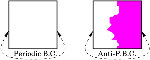
Figure 2: Domain-wall for the ferromagnetic case: the shaded region represents the spins that have flipped.

This suggests we consider the scaling ${\Delta}_{g}\simeq L_{g}^{d-1}$ when $g\to\infty$. We thus define $x_{g}$ as ${\Delta}_{g}/L_{g}^{d-1}$ and hope for a LDP of the type

$$p(x_{g}=t)\simeq e^{-N_{g}f(t)}\ .$$ (28)

Let’s rewrite the autonomous Eq. LABEL:MK-main-ds for $x_{g}$ as:

$$\begin{split}&x_{g+1}=\frac{1}{b}\sum\limits_{k=1}^{b}\\ &\mbox{sign}\Big{[}x_{g}(1,k)x_{g}(2,k)\Big{]}\min\{|x_{g}(1,k)|,|x_{g}(2,k)|\}\ .\end{split}$$ (29)

Unlike the case in one dimension, it is impossible to apply the technique of distribution functions because of the sum over $k$ terms; similarly, a Fourier transformation is useless because of the minimization. Nevertheless, some progress can be made by noting that the right side of Eq. 29 is a partial mean of $x_{g}(\alpha,k)$, $\alpha=1,2$. Then one can show that if $x_{g}$ satisfies the LDP with LDF $f(t)$, then so does $x_{g+1}$: once a LDP is formed, it is conserved. Empirically, the LDP turns out to be exactly as expected in Eq. 28. Thus, we believe a limit $f(t)=-\lim N_{g}^{-1}\ln p_{g}(x_{g}=t)$ as $N_{g}\to\infty$ exists. Clearly, the LDF isn’t universal; it depends on the initial distribution $p_{0}$ of $x_{0}$.

To obtain an analytical estimate of $f(t)$, we notice that as $b\to\infty$ the LDP should be formed after just one generation. An approximation $f_{a}(t)$ for the LDF $f(t)$ is then

$$f_{a}(t)=\frac{1}{2}\max\limits_{\lambda}\left\{\lambda t-\ln\Big{[}4\int dse^{s\lambda}p_{0}(s)\int\limits_{|s|}^{\infty}dvp_{0}(v)\Big{]}\right\}$$ (30)

where the argument of the logarithm is the characteristic function of $\mbox{sign}(x_{0}(1)x_{0}(2))\min\{|x_{0}(1)|,|x_{0}(2)|\}$. This formula arises from the direct application of Cramér’s theorem for Eq. 29 with $g=0$, regarding the quantities $\mbox{sign}(x_{0}(1)x_{0}(2))\min\{|x_{0}(1)|,|x_{0}(2)|\}$ as the i.i.d. variables (recall that they live on different branches).

How good is this approximation, and in particular does it become exact at large $b$? Note that the LDF (30) is $b$-independent because we took $b\to\infty$ and we expect in fact $f_{a}(t)$ to be the limiting value of $f(t)$ as $b\to\infty$. A series of numerical simulations were carried out in order to quantify the large $b$ approximation. We used the bimodal distribution $J_{ij}=\pm 1$:

$$p_{0}(J)=\frac{1}{2}(\delta(J-1)+\delta(J+1))\ .$$ (31)

The evaluation of Eq. 30 for $|t|\leq 2$ then gives:

$$f_{a}(t)=\frac{1}{2}\left[-\ln 2+\ln\sqrt{4-t^{2}}-\frac{t}{4}\ln\left(\frac{2-t}{2+t}\right)\right]$$ (32)

which is even as it must; one also has $f_{a}(t)=+\infty$ for $|t|>2$ which is good since it also holds necessarily for the exact $f(t)$.

Figure 3: Domain-wall LDF for the Migdal-Kadanoff lattices when $J_{ij}=\pm 1$. Displayed are data for $b=4$, $b=10$, and the theoretical $b=\infty$ prediction.

The simulations revealed a rapid convergence with generations of the large deviations functions to their limits: $g=5$ was enough to nearly reach machine precision even when $b=4$. Furthermore, as illustrated in Fig. 3, the discrepancy $\delta f(t)$ between the theoretical prediction $f_{a}(t)$ and the numerically determined LDF decreased with increasing $b$ (a few percent for $b=10$ to fractions of a percent for $b=50$). The numerical analysis of $\delta f$ suggests that the corrections are of order $b^{-5/8}$. The behaviour of $b^{0.625}\delta f(t)$ is shown in Fig. 4 for several values of $b$. Naturally, it would be of interest to understand the origin of this exponent. It is also interesting to note that the range of $t$ is bounded, $-2\leq t\leq 2$, but that the derivative of $f$ at these limit points is finite, in contrast to what happened in the one-dimensional model.

Figure 4: Rescaled difference between the $b$ finite and $b=\infty$ LDF for domain-wall energies within the $J_{ij}=\pm 1$ MK model.

3.3 Ground-state energies

The study of $E_{0}$ is more complicated as it has no autonomous recursion equation: we must follow the joint distribution of $\Sigma$ and $\Delta$. Recall that

$$E_{0}=(\Sigma-\Delta)/2\ ;$$ (33)

since ${\Delta}_{g}$ scales as $L_{g}^{d-1}$ whereas ${\Sigma}_{g}$ scales as $L_{g}^{d}$, the $\Delta$ term in Eq. 33 can be neglected in the study of large deviations. Thus, the large deviations of $\Sigma$ and of $E_{0}$ coincide, allowing us to focus hereafter on $\Sigma$.

We define the intensive variable ${\xi}_{g}={\Sigma}_{g}/N_{g}$ and rewrite Eq. LABEL:MK-main-ds as:

$$\begin{split}&{\xi}_{g+1}=\frac{1}{b}\sum\limits_{k=1}^{b}\Bigl{[}\frac{1}{2}({\xi}_{g}(1,k)+{\xi}_{g}(2,k))\\ &-\frac{1}{2^{g+1}}\max\{|x_{g}(1,k)|,|x_{g}(2,k)|\}\Bigr{]}\ .\end{split}$$ (34)

A LDP is expected as $N_{g}\to\infty$:

$$p(\xi_{g}=t)\sim\exp(-N_{g}f(t))\ .$$ (35)

Note that $\overline{\Sigma}$, the disorder average of $\Sigma$, has a non-zero mean value; it can be written in terms of the statistics of the $x$ via iteration of Eq. LABEL:MK-gs-main-n:

$$\overline{\xi_{g+1}}=-\sum\limits_{p=0}^{g}\frac{1}{2^{p+1}}\overline{\max\{|x_{k}(1)|,|x_{k}(2)|\}}$$ (36)

where the index $p$ labels generations. This identity leads us to guess that the statistics of ${\xi}$ is determined entirely by that of $x$. Indeed, it is possible to write down explicitly ${\xi}_{g+1}$ in terms of the $x_{p}$, $0\leq p\leq g$:

$$\begin{split}&{\xi}_{g+1}=\\ &-\frac{1}{2}\sum\limits_{p=0}^{g}\frac{2^{-p}}{b{(2b)}^{g-p}}\sum\limits_{m=1}^{b{(2b)}^{g-p}}\max\{|x_{p}(1,m)|,|x_{p}(2,m)|\}\end{split}$$ (37)

where the different $x$’s have been regrouped according to their generation number. Evidently the terms within the sum over $m$ are independent, but the terms for different generations are correlated: indeed, each $x_{p+1}$ is a sum over a sub-set of the $x_{p}$’s. Thus the problem hasn’t really become easier: instead of the joint distribution of $\xi$ and $x$, we are obliged to consider the joint distribution of the $x_{p}$ at all $p\leq g$. On the other hand it is reasonable to expect weak cross-generation correlations for $b\to\infty$. This suggests the approximation of independent generations: take all the terms in Eq. LABEL:MK-gs-main-xn to be uncorrelated! Such an approximation leads to the estimate $\tilde{f}(t)$ of the LDF:

$$\tilde{f}(t)=\frac{1}{2}\sum\limits_{p=0}^{\infty}\frac{1}{N_{p}}\ln M^{\max}_{p}\left(\frac{t}{2^{p+1}N_{p}}\right)\ .$$ (38)

In this equation, $M_{p}^{\max}$ represents the characteristic function for $\max\{|x_{p}(1)|,|x_{k}(2)|\}$. To actually compute $\tilde{f}$, we started with the numerically determined distribution of the $x_{p}$ and performed the sum in the series as far as possible and then estimated the remaining part from asymptotics.

Numerical simulations were carried out to determine the distributions of $\Sigma$ and of the $x_{p}$. As before, we used the bimodal $J_{ij}=\pm 1$ distribution of couplings. Although this time it was much harder to compute the distribution of $\Sigma$ when $g$ grew, again a good convergence in $g$ was found in 5 to 6 generations; this is illustrated in Fig. 5. Note that since we are dealing with the $J_{ij}=\pm 1$ model, we clearly have $-2\leq\xi\leq 0$ at large $g$, but in fact the upper limit is not reached for finite $b$. Also, when $g$ is finite, the ranges for $\xi$ are slightly different. Finally, as $g$ grows, it is difficult to follow the far tail of the distribution of $\Sigma$ because the probabilities there become extremely small. These different effects are responsible for the cut-offs in the curves we show. As another general remark, consider the ferromagnetic limit. The probability of having no frustration in the MK lattice is bounded from below by $2^{-N_{g}}$; thus necessarily $f(-2)$ is finite whereas $f(t)=\infty$ as soon as $t<-2$.

Figure 5: Convergence of the ground-state energy density LDF with the number of generations when $b=4$ in the $J_{ij}=\pm 1$ MK model.

Figure 6: Ground-state energy density LDF when $b=4$ in the $J_{ij}=\pm 1$ MK model: comparison of the independent generations approximation (“theory”) and simulations.

How does the estimate of $f$ (obtained from the data at the largest $g$ we can handle) compare to $\tilde{f}$, the prediction of the independent generations approximation?

Figure 7: Ground-state energy density LDF when $b=10$ in the $J_{ij}=\pm 1$ MK model: comparison of the independent generations approximation (“theory”) and simulations.

The results for $b=4$ and 10 are shown in Figs. 6 and 7. The discrepancy between “theory” and numerics is larger than it was for $\Delta$ but the error does decrease slowly as $b\to\infty$, giving evidence that the independent generations approximation becomes exact as $b\to\infty$.

4 The Random Energy Model

The simplest model of spin glasses is the Random Energy Model (REM) Derrida80 . In a system with $N$ spins there are $2^{N}$ possible assignements of the spins, leading to $2^{N}$ possible energy levels. The framework of the REM is to consider that these energies are independent. The usual choice is for each energy level to have the probability density

$$p_{N}(u)=\frac{1}{\sqrt{\pi N}}\exp(-u^{2}/N)$$ (39)

whose integrated distribution is

$$q_{N}(u)=\int_{u}^{\infty}\frac{dv}{\sqrt{\pi N}}\exp(-v^{2}/N)\ .$$ (40)

The ground-state energy $E_{0}$ for this system is given by:

$$E_{0}=\min\{x_{1},\ldots,x_{2^{N}}\}\ .$$ (41)

As such, $E_{0}$ has follows Gumbel Gumbel58 distribution. However, we are mainly interested in large deviations that are associated with events where $E_{0}$ is far from its typical value. Noting that the $N$ dependence of $p_{N}$ is chosen so that $E_{0}$ scales linearly with $N$ in the large $N$ limit, we thus consider $e_{0}=E_{0}/N$:

$$e_{0}=\frac{1}{N}\min\{x_{1},\ldots,x_{2^{N}}\}\ .$$ (42)

Since the $x_{i}$ are independent, the integrated distribution of $e_{0}$ is:

$$P\{e_{0}\geq t\}=\Big{[}P\{x_{1}\geq tN\}\Big{]}^{2^{N}}=q_{N}^{2^{N}}(tN)$$ (43)

giving

$$p(e_{0}=t)=N2^{N}q_{N}^{2^{N}-1}(tN)p_{N}(tN)\ .$$ (44)

The asymptotic behavior of these quantities is easily evaluated. For $t<-\sqrt{\ln 2}$, we have

$$p(e_{0}=t)\simeq e^{-N(t^{2}-\ln 2)}$$ (45)

in agreement with the fact that the typical value of $e_{0}$ is $-\sqrt{\ln 2}$. When $-\sqrt{\ln 2}<t<0$, the nature of the scaling is different :

$$\ln p(e_{0}=t)\simeq-e^{-N(t^{2}-\ln 2)}\ .$$ (46)

The scaling at $t<-\sqrt{\ln 2}$ can be understood by considering the probability that just one of the $2^{N}$ energies is anomalously low. On the contrary, the case $t>-\sqrt{\ln 2}$ follows by imposing that all $2^{N}$ energies are a bit high. We learn from this example that the “normal” scaling of Eq. 2 does not always arise, one may have one type of LDP for $t<\overline{e_{0}}$ and another for $t>\overline{e_{0}}$.

5 The Sherrington-Kirkpatrick model

The Sherrington-Kirkpatrick SherringtonKirkpatrick75 model (hereafter SK) is the mean field limit of spin glasses where all $N$ spins are connected to one another. The Hamiltonian is

$$H_{J}=-\sum_{i<j}J_{ij}S_{i}S_{j}$$ (47)

the $S_{i}=\pm 1$ are Ising spins and the couplings $J_{ij}$ are Gaussian random variables of zero mean and variance $1/N$. (This scaling ensures a good thermodynamic limit, the free energy scaling linearly with $N$.) We focus on the statistics of the ground-state energy $E_{0}$ of this Hamiltonian. For a given sample, $E_{0}$ can be determined by combinatorial optimization techniques; we have used a genetic algorithm HoudayerMartin99b which finds $E_{0}$ with a high level of reliability when $N$ is not too large. This is true for the SK model and also for the other models we shall consider further on. In all these cases, we restrict ourselves to $N$ values where the true $E_{0}$ is almost certainly obtained. We then compute the statistics of $E_{0}$ for a number of different system sizes $N$ and then attempt to extrapolate to the large $N$ limit.

5.1 Limiting distribution

Before examining the large deviations of $E_{0}$ in the SK model, let’s first discuss its limiting distribution. The mean of $E_{0}$ scales linearly with $N$, and has a variance that grows, but one may expect the distribution of $E_{0}$ to have a limiting shape. To study this, one introduces the scaling variable

$$X_{J}={\frac{E_{0}-\overline{E_{0}}}{\sigma(E_{0})}}$$ (48)

where $\overline{E_{0}}$ is the disorder average of $E_{0}$ and $\sigma(E_{0})$ its standard deviation. Bouchaud et al. BouchaudKrzakala03 studied the distribution of $X_{J}$, finding that, for most models of spin glasses it becomes Gaussian as $N\to\infty$. However in the case of the SK, the behavior was clearly non-Gaussian. Since $E_{0}$ is an extreme statistic, being the minimum of $2^{N}$ energies, it is natural to ask whether the distribution of $E_{0}$ falls into a known universality class. There are three standard universality classes for the minimum of uncorrelated variables Gumbel58 : (1) Gumbel for unbounded distributions whose tail decreases faster than any power; (2) Fisher-Tippett-Frechet for distributions whose tail decreases as a power; (3) Weibull for distributions with cut-offs. The REM clearly falls into the first class. Interestingly, the SK does not fall into any of these three classes BouchaudKrzakala03 ; PalassiniHouches03 , leaving open the question of the universality class appropriate for its $E_{0}$.

Recently a new universality class has been uncovered by Tracy and Widom TracyWidom99 : in the context of random matrix theory, they found the limiting distribution of the largest eigenvalue of an $N\times N$ random matrix when $N\to\infty$. This distribution is believed to be universal, and has already been applied to a number of different systems. Note that we are dealing now with the maximum of a large number of correlated random variables; furthermore, because of the minus sign in Eq. 47, we have to consider in fact $(-1)$ times this largest eigenvalue when comparing to $E_{0}$ (note that this changes the sign of the skewness). We refer to the distribution of this quantity within the Gaussian Orthogonal Ensemble as the Tracy-Widom (TW) distribution.

How does the distribution of $E_{0}$ compare with that of TW? We find that the agreement is surprizingly good. In Fig. 8 we have plotted the TW distribution as a continuous curve and our SK data when $N=50,100,150$. In the inset we compare the two distributions directly; the naked eye sees no difference between the two. In the main part of the figure, we zoom on the tails, displaying the data on a logarithmic scale; then definite deviations appear on the left wing.

Figure 8: Comparison of the Tracy-Widom distribution to that of the Sherrington-Kirkpatrick model at $N=50,100,150$. Data shown are on a logarithmic scale (and on a linear scale for the inset); $X_{J}$ is defined in Eq. 48.

At a more quantitative level, we have also compared the values of skewness $S$ and kurtosis $K$ of the TW and SK distributions. Our estimations are summarized in Table 1.

Table 1: Skewness (S) and Kurtosis (K) for the TW distribution and for that of $E_{0}$ in the SK model (numerical estimates are for $N=50$, $100$, and $150$).

	$TW$	$SK_{50}$	$SK_{100}$	$SK_{150}$
$S$	$-0.293$	$-0.43$	$-0.42$	$-0.41$
$K$	$0.165$	$0.41$	$0.36$	$0.39$

We find a “large” disagreement; clearly the discrepancy seen in the tail of Fig. 8 affects these cumulants, in fact all the more that they are of higher order. Since at least the SK skewness is numerically stable and quite different from the TW skewness, we feel that our data indicate that the two distributions, though very close, are in fact distinct. Thus TW does not give us the universality class for SK.

On the theoretical side, what possible justification could be given for $E_{0}$ to be described by TW since $E_{0}$ is a minimum over $2^{N}$ variables whereas in the TW matrix problem one considers the extremum of $N$ variables? One possible answer resides in the spherical approximation to the SK model. Kosterlitz et al. KosterlitzThouless76 solved the SK model in that approximation and showed that in the limit $T\to 0$, the Boltzmann weight becomes dominated by the largest eigenvalue of the interaction matrix $J_{ij}$; this then leads to a TW distribution for $E_{0}$ in that model. Given this result, it would be good to understand why the spherical approximation seems to be so good for the shape of the distribution of $E_{0}$ yet gives a very poor approximation for the ground-state energy density ($-1.0$ to be compared with the actual value of $-0.7633$).

To push further the point that we do not believe the two distributions to be identical, consider the following fact. If we consider the maximum eigenvalue of a random symmetric matrix, the result of TW shows that the mean shifts with $N$ and the standard deviation grows with $N$. Translating into the variable $E_{0}$, the correspondence with random matrix theory would predict that

$${\overline{E_{0}}}-Ne_{0}^{*}\simeq N^{1/3}$$ (49)

and

$${\overline{E_{0}^{2}}}-{\overline{E_{0}}}^{2}\simeq N^{2/3}$$ (50)

where $e_{0}^{*}$ is the thermodynamic limit of ${\overline{E_{0}}/N}$. The first equation is in agreement with what happens in the SK model PalassiniThesis ; BouchaudKrzakala03 , but the standard deviation does not at all grow as $N^{1/3}$ but much more slowly BouchaudKrzakala03 ; PalassiniHouches03 .

5.2 Large deviations

Still staying within the SK model, we now turn to the large deviations of $e_{0}=E_{0}/N$. The central question is whether there is a LDP. A naive expectation would be that

$$p_{N}(e_{0})\simeq e^{-Nf(e_{0})}$$ (51)

but our data do not follow such a scaling. By considering the dependence of $\ln p_{N}(e_{0})$ on $N$, our data suggest two quite distinct power laws in $N$: $N^{1.5}$ when $e_{0}>{\overline{e_{0}}}$ and $N^{1.2}$ when $e_{0}<{\overline{e_{0}}}$. We thus define two LDF:

$$f_{>}(e_{0})=-\frac{\ln\left[p_{N}(e_{0})/N^{0.75}\right]}{N^{1.5}}$$ (52)

in the first case and

$$f_{<}(e_{0})=-\frac{\ln\left[p_{N}(e_{0})/N^{0.6}\right]}{N^{1.2}}$$ (53)

in the second. The additional rescaling in the log has no effect on the large $N$ scaling, but we found it to reduce finite size effects; note that the motivation for this term comes from Bahardur-Rao theorem given in Section 2. We plot in Fig. 9 these two functions modulo a shift of the $x$ axis.

It is not surprizing that the exponent found for $f_{<}$ is less or equal to 1.5. Indeed, consider for instance a sample with $e_{0}\leq{\overline{e_{0}}}$. Now change the sign of $O(N^{1.5})$ $J_{ij}$ that are unsatisfied; this will “cost” a probability $O(\exp\left[-AN^{1.5}\right])$. With this change, we have $e_{0}\to e_{0}-\delta$ where $\delta$ is finite, i.e., the desired result. The fact that the exponent turns out to be smaller than 1.5 probably comes from the fact that there are many ways to choose these $O(N^{1.5})$ $J_{ij}$ whereas the argument uses only one such choice.

Figure 9: Large Deviations Functions $f_{<}$ and $f_{>}$ for the Sherrington-Kirkpatrick model when $N=30$, $50$, …, $300$.

Because we are restricted to $N$ not very large, we cannot exclude the possibility that we are seeing effective exponents and that a different scaling arises at larger $N$. (In contrast to the MK case, the large deviations become much more difficult to measure when $N$ grows and our algorithm for determining $E_{0}$ also breaks down at large $N$.) Nevertheless, since our scalings work well, the data strongly suggest that there really are two different exponents for $e_{0}<e_{0}^{*}$ and $e_{0}>e_{0}^{*}$, just as in the REM.

5.3 Very large deviations

In the one-dimensional example of Section 2.1 and in the MK model, the ferromagnetic limit arose when $e_{0}\ll e_{0}^{*}$. In the SK model, the absence of frustration requires constraining $O(N^{2})$ $J_{ij}$ and changes the scaling of $e_{0}$ which becomes $O(N^{1/2})$. Clearly such deviations are far rarer than simply having $e_{0}\ll e_{0}^{*}$. Because of this, we are limited in our numerical study to even smaller $N$ values than before. Nevertheless, we have investigated these deviations by considering the probability distribution of $e_{0}/N^{1/2}$. We find

$$p_{N}(e_{0}/N^{1/2})\simeq Ne^{-N^{2}f(e_{0}/N^{1/2})}$$ (54)

with a very large deviations function (VLDF) $f$ displayed in Fig. 10. (To reduce finite $N$ effects, we have in fact used $e_{0}-\overline{e_{0}}$ rather than $e_{0}$ itself, but this does not change the asymptotics.) We see that for positive arguments, the estimates for $f$ increase with $N$ which is compatible with the expectation that $f(t)=\infty$ when $t>0$. For negative arguments, the data collapse quite well, justifying the VLDP proposed in Eq. 54.

Figure 10: Very Large Deviations Function for the Sherrington-Kirkpatrick model: data for $40\leq N\leq 100$.

6 Other spin-glass models models

Most probably, the subtleties of the SK model arise from the fact that all spins are connected to one-another. In more realistic models, spins interact with just a few neighbors. We thus return to models of the type described by the Hamiltonian in Eq. 22, and now impose the number of neighbors to be fixed and constant. The two standard classes of models that do that are the Edwards-Anderson EdwardsAnderson75 model on square or cubic lattices and the mean field fixed connectivity models DominicisGoldschmidt89 . At present, no analytical tools are available for treating large deviations, so we resort to a purely numerical analysis. In what follows, the disorder variables $J_{ij}$ of Eq. 22 are i.i.d. Gaussian random variables of zero mean and unit variance.

6.1 Euclidean models

We first look at the LDF of $e_{0}$ for the Edwards-Anderson model with Gaussian couplings in two and three dimensions. In the case of finite dimensional lattices, we know that the variance of $E_{0}$ grows linearly with $N$, and most probably the distribution of $E_{0}$ is Gaussian WehrAizenman90 . This suggests that the terms contributing to the ground-state energy are nearly independent, just as in the MK case. Then the functions

$$f_{N}(e_{0})=\frac{-\ln\left[p_{N}(e_{0})/N^{1/2}\right]}{N}$$ (55)

should converge as $N\to\infty$. We first checked this on our $3\leq L\leq 10$ data in the two-dimensional ($d=2$) case. Under the hypothesis that the finite size corrections are $O(1/N)$, we extract the limiting function $f_{\infty}$ for $N\to\infty$. This function is shown in Fig. 11 as a continuous curve. The LDF is asymmetric, increasing more rapidly on the right than on the left. We also show our data for the $f_{N}$, showing that the scaling in Eq. 55 works well. The $d=3$ case is displayed as an inset; note that the LDF is more symmetric than for $d=2$. Also, the convergence of $f_{N}$ to $f_{\infty}$ again goes as $O(1/N)$.

Figure 11: Large Deviations Function in the Edwards-Anderson model with Gaussian couplings in $d=2$. The solid line is the limiting curve for $N\to\infty$. Inset: the $d=3$ case.

6.2 Fixed connectivity random graphs

We now focus on random graphs that are of fixed connectivity $z$ at each site. Such graphs can be generated by the following simple algorithm. First construct $N$ vertices, then successively add edges to the graph by randomly connecting sites whose current connectivity is less than $z$. This process can be made more efficient by keeping a list of all the candidate sites. The size of this list decreases; if it reaches $1$, the construction has to be abandoned and restarted. In practice such a failure does not occur very often.

Just as in the Euclidean case, we find the simple scaling

$$p_{N}(e_{0})\simeq A\sqrt{N}e^{-Nf(e_{0})}\ .$$ (56)

Thus as in the MK case, we are closer to a sum of i.i.d. random variables than to a minimum of independent variables.

Figure 12: Large Deviations Function for fixed connectivity random graphs when $z=10$. Inset: the case $z=3$.

In Fig. 12 we display the LDF for the case $z=10$; the inset is for $z=3$. We see that the convergence to the large $N$ limit is quite good, leading to an envelope curve. It should be clear that the two functions displayed are distinct: the case $z=3$ is a bit more symmetric than the case $z=10$.

7 Conclusions

We have investigated the large deviations of the ground-state energy $E_{0}$ in several Ising spin-glass models. There are two extreme cases: (1) $E_{0}$ is the sum of independent random variables (as in a one dimensional lattice); (2) $E_{0}$ is the minimum of a large number of independent random variables (as in the Random Energy Model). The case of the Sherrington-Kirkpatrick model led to a behavior intermediate between these two extremes. However, the other spin-glass models we considered, all of which have finite connectivity, resemble closely the first case. This was particularly patent for the hierarchical lattice models where high quality numerical computations were possible as well as analytical estimates.

We also pointed out that the large deviations function is not universal; in particular, its tails depends very much on the far distribution of the disorder variables $J_{ij}$. This leads one to ask whether there is any universality in large deviations functions. This question is all the more interesting that Brunet and Derrida BrunetDerrida00 found the large deviations function for a directed polymer in a random medium to be universal; furthermore, that function is the same as the one describing infinitesimal deviations in their system. To have this kind of universality in spin glasses, the deviations must not affect much the values taken by the $J_{ij}$; for us, this seems possible only in the Sherrington-Kirkpatrick model. More precisely, we believe that the regime $E_{0}=O(N)$ in that model is universal (independent of the details of the $J_{ij}$); this is to be contrasted with the ferromagnetic limit where clearly the large deviations function is not universal.

Many questions surrounding these issues are still very open; let us list a few. (0) What are the analytical properties of the large deviation function, and when is it related to the distribution of infinitesimal deviations? (1) When the large deviations function is finite, we found a quite smooth convergence of our finite $N$ estimates to a limiting curve; is this convergence uniform? (2) What is the distribution of the disorder variables $J_{ij}$ when $e_{0}$ deviates from its typical value? (3) In the ferromagnetic limit, do the regions with frustration phase separate out? (We believe not.) Clearly, numerical analysis is not a good tool to tackle most of these questions. Fortunately, there is good reason to believe that Migdal-Kadanoff lattices provide a good framework to address these questions; we hope that analytical results will be derived in the near future for such spin-glass models.

Acknowledgements – We thank A. Pagnani for his help throughout this project and C. Tracy for providing us with his Mathematica program for generating the TW distribution. We also thank O. Bohigas, J.-P. Bouchaud, B. Derrida, E. Marinari, M. Mézard, R. Monasson and G. Parisi for their critical comments. This work was supported in part by the European Community’s Human Potential Programme (contracts HPRN-CT-2002-00307 for DYGLAGEMEM and HPRN-CT-2002-00319 for STIPCO).

References

- (1) M. Lifshitz, S. A. Gredeskul, and L. A. Pastur, Introduction to the theory of disordered systems (Wiley, New York, 1988).
- (2) B. Derrida, Phys. Rev. Lett 45, 79 (1980).
- (3) B. Derrida, J. Phys. Lett. (France) 46, 401 (1985).
- (4) A. Bovier and I. Kurkova, Markov Processes Rel. Fields 9, 209 (2003).
- (5) D. Sherrington and S. Kirkpatrick, Phys. Rev. Lett. 35, 1792 (1975).
- (6) M. Talagrand, Probability Theory and Related Fields 117, 303 (2000).
- (7) W. Feller, An introduction to probability theory and its applications (John Wiley and sons, New York, NY, 1950).
- (8) J. Bucklew, Large deviations techniques in decision, simulation, and estimation (John Wiley and sons, New York, NY, 1990).
- (9) E. J. Gumbel, Statistics of Extremes (Columbia University Press, NY, 1958).
- (10) B. W. Southern and A. P. Young, J. Phys. C 10, 2179 (1977).
- (11) A. N. Berker and S. Ostlund, J. Phys. C: Solid State Phys. 12, 4961 (1979).
- (12) A. J. Bray and M. A. Moore, in Heidelberg Colloquium on Glassy Dynamics, Vol. 275 of Lecture Notes in Physics, edited by J. L. van Hemmen and I. Morgenstern (Springer, Berlin, 1986), pp. 121–153.
- (13) D. S. Fisher and D. A. Huse, Phys. Rev. Lett. 56, 1601 (1986).
- (14) J. Houdayer and O. C. Martin, Phys. Rev. Lett. 83, 1030 (1999), cond-mat/9901276.
- (15) J.-P. Bouchaud, F. Krzakala, and O. C. Martin, Phys. Rev. B 68, 224404 (2003), cond-mat/0212070.
- (16) M. Palassini, (2003), lecture at Les Houches.
- (17) C. Tracy and H. Widom, Statistical Physics on the Eve of the 21st Century 230 (1999).
- (18) J. Kosterlitz, D. Thouless, and R. Jones, Phys. Rev. Lett. 36, 1217 (1976).
- (19) M. Palassini, Ph.D. thesis, Scuola Normale Superiore, Pisa, Italy, 2000.
- (20) S. F. Edwards and P. W. Anderson, J. Phys. F: Met. Phys. 5, 965 (1975).
- (21) C. De Dominicis and Y. Goldschmidt, J. Phys. A 22, L775 (1989).
- (22) J. Wehr and M. Aizenman, J. Stat. Phys. 60, 287 (1990).
- (23) E. Brunet and B. Derrida, Phys. Rev E 61(6), 6789 (2000).