Monitoring of Orientation in Molecular Ensembles by Polarization Sensitive Nonlinear Microscopy
Véronique Le Floc’h, Sophie Brasselet, Jean-François Roch, Joseph Zyss
Laboratoire de Photonique Quantique et Moléculaire (UMR 8537),
Institut d’Alembert (IFR 121), École Normale Supérieure de Cachan
61, avenue du Président Wilson, 94235 Cachan Cedex, France

We present high resolution two-photon excitation microscopy studies combining two-photon fluorescence (TPF) and second harmonic generation (SHG) in order to probe orientational distributions of molecular ensembles at room temperature. A detailed polarization analysis of TPF and SHG signals is used in order to unravel the parameters of the molecular orientational statistical distribution, using a technique which can be extended and generalized to a broad variety of molecular arrangements. A polymer film containing molecules active for TPF and/or SHG emission is studied as a model system. Polarized TPF is shown to provide information on specific properties pertaining to incoherent emission in molecular media, such as excitation transfer. SHG, being highly sensitive to a slight departure from centrosymmetry such as induced by an external electric field in the medium, complements TPF. The response of each signal to a variable excitation polarization allows investigation of molecular behavior in complex environments which affect their orientations and interactions.

I. Introduction

Multi-photon microscopy has amply demonstrated its assets in the study of broad variety of physical and biological phenomena. Among the effects arising from two-photon excitation, two-photon fluorescence (TPF) has been at the focus of much attention for many reasons.[1] Contrary to linear fluorescence, for which background noise rejection requires the implementation of confocal detection, TPF exhibits an intrinsic high spatial resolution due to the built-in quadratic power dependence on the excitation intensity. In addition, the use of infrared excitation minimizes both optical damage and background scattering in complex samples such as living cells.[2] This method has shown significant advantages in imaging of complex biological environments down to the single molecule level.[3] In parallel, developments in molecular engineering have lead to the design of chemical probes exhibiting very high two-photon absorption cross sections.[4, 5] Such results have triggered important advances in the field of two-photon imaging and other processes such as optical limiting. Finally, multi-photon microscopy techniques have been extended to a larger variety of nonlinear optical processes such as three-photon induced fluorescence, as well as second- and third-harmonic frequency generation both in far-field and near-field microscopies.[6, 7, 8, 9]

Second harmonic generation (SHG) is the result of coherent emission from anharmonic oscillators upon two-photon excitation. At macroscopic scale, SHG emission vanishes in centrosymmetric media, since the $\chi^{(2)}$ related nonlinear susceptibility is an odd-rank tensor. In molecular media, non-centrosymmetric ordering is traditionally obtained by electric field poling of intrinsically non-centrosymmetric molecules, such as dipolar $\pi$-conjugated systems functionnalized with adequate acceptor and donor groups. [10] As SHG is highly sensitive to even a slight departure from centrosymmetry in molecular media, this effect has been widely used to study surface and interface properties in physics and chemistry, with monolayer sensitivity.[11, 12] SHG signals have also been measured in artificial vesicles,[13] live cells,[14] and in biological membranes in the presence of an electric potential.[15]

In this work, we study TPF and SHG in model molecular systems and take advantage of the specific properties and complementarities of these nonlinear processes. The main difference between them lies in the coherent nature of the emitted signals and their relative spectral features. Contrary to fluorescence, which is based on the time-delayed relaxation of a radiative level, off-resonant SHG occurs instantaneously upon excitation. Furthermore, the fluorescence emission is affected by a Stokes shift, whereas SHG occurs at half the incident wavelength and is phase-correlated with the excitation field at the fundamental frequency. These specific features allow one to distinguish them either spectrally or temporally.[16]

The main advantage of combining the two processes lies in their respective anisotropy sensitivity to molecular orientation under polarized excitation. In a centrosymmetric medium, SHG vanishes while TPF is always present and can be anisotropic if the molecular orientational distribution symmetry is axial.[17] Moreover, SHG appears in a polar medium, and is intrinsically anisotropic. The difference between these two effects is due to the distinct symmetry properties of the tensorial susceptibilities that are involved, TPF and SHG being described by even and odd order tensors respectively. The related macroscopic susceptibilities reflect both molecular-scale and macroscopic-scale arrangement properties, such as orientational distribution. Measuring TPF and SHG anisotropies is therefore a direct way to probe a given molecular organization in a molecular ensemble that is either naturally ordered, or that has been subject to the application of an external perturbation, such as an electric field,[18, 19] a coherent combination of optical excitations,[20] or a combination of these.[21] Complex tensorial distributions can be unravelled using such approaches.[22]

In order to fulfill the symmetry requirements discussed above, we chose a model medium consisting of an amorphous polymer matrix doped with fluorescent and/or dipolar nonlinear active chromophores. Macroscopic centrosymmetry breaking of the medium is induced by electric field orientation of these chromophores, using planar geometry suited to the two-photon microscopy experimental setup. Applying an external electric field results in a controllable external degree of freedom used to monitor the molecular order symmetry. Furthermore, the reflection geometry of the inverted microscopy configuration used in this work allows one to measure both TPF and SHG signals without any dependence on the coherence length of the nonlinear field propagation. The experimental configuration presented here can be easily applied to a variety of situations such as in biological membrane studies where electric potentials might induce the orientation of a molecular probe. Such studies can be potentially down-scaled to a low number of molecules and even to single macromolecules, where interactions at the molecular level or global conformational changes can affect the collective emission anisotropy properties.

We present a detailed analysis of the orientational molecular ordering in the sample using both TPF and SHG processes. We show that the rotating-polarization analysis can bring additional informations that might be hidden in ratiometric anisotropy measurements. This analysis can be straightforwardly adapted to a large variety of environments, and to dynamical effects.[19] Accounting for the instrumental features of inverted microscopy, with high numerical aperture (N.A.) objectives collecting light at wide angles of emission, we show that a simple model allows one to retrieve information on localized dipole orientations. As we demonstrate in this work, the analysis of nonlinear anisotropies requires therefore particular attention to the polarization state at the focus of a high N.A. objective and the definition of a calibration procedure. In the following sections, we discuss the optical properties of both TPF and SHG processes in random and ordered media, taking into account the influence of excitation transfer between chromophores.

II. Experimental section

A. Sample Preparation

The samples, studied at room temperature, contain active chromophores, either 4-dicyanomethylene-2-methyl-6-(p-(dimethylamino)styryl)-4H-pyran (DCM) or 4-(N-ethyl-N-(2-hydroxyethyl))amino-4’-nitro-azobenzene (Disperse Red 1, DR1). The DCM chromophore exhibits a high fluorescence quantum yield and a non negligible molecular quadratic polarizability $\beta$.[23] The DR1 chromophore, which has been extensively studied for its intrinsic high quadratic nonlinear efficiency,[24] is not fluorescent because of quenching by fast photoisomerization. Both chromophores exhibit a large permanent dipole moment which enables electric field orientation.

The molecules are dispersed with a maximum concentration of $10\%$ by mass in a high $T_{\textrm{g}}$ (120^∘C) polymer matrix of polymethyl-methacrylate (PMMA), which is not cured after deposition. The polymer films are then deposited by spincoating either on a microscope slide or on an electrode substrate.[25] In order to achieve electric field alignment in the plane of the sample, we use a set of gold transverse planar electrodes of 50 nm thickness, separated by a gap of 10 $\mu$m, as represented in Figure 1. The electrodes are fabricated by photo-lithographic patterning of UV sensitive photoresists on the gold layer, which is deposited by sputtering on a microscope slide covered with a 100 nm PMMA adhesion layer. The thickness of the active PMMA-dye layer is of the order of 100 nm, in which the active molecules are expected to orientate perpendicular to the electrodes in the sample plane.

B. Experimental Setup

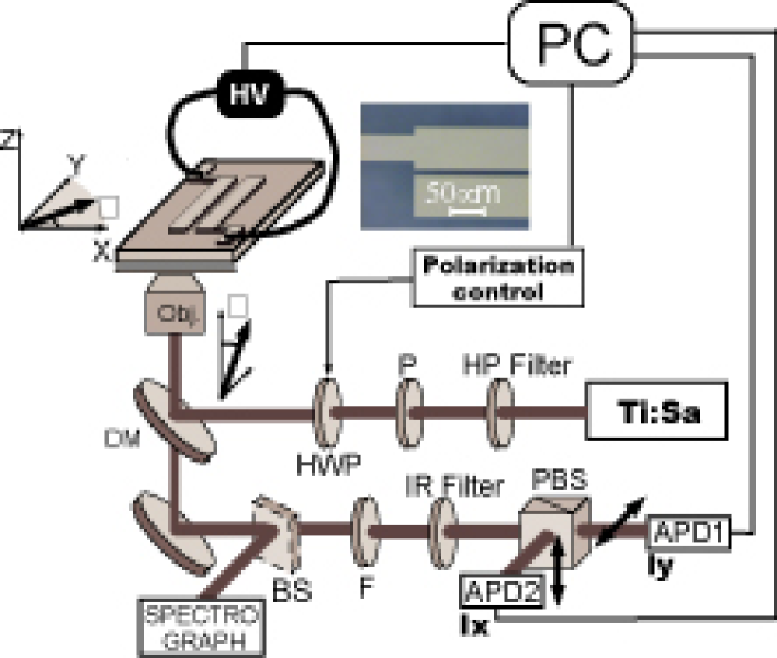
Figure 1: Nonlinear microscopy setup: HP filter: high pass filter which rejects visible light; P: polarizer; HWP: rotating half-wave plate; Obj: microscope objective ($\times 60$, NA=1.4); DM: dichroic mirror; F: interference filter selecting either the SHG signal at 493 nm or the TPF signal at 580 nm; IR filter: filter rejecting the residual incident (near IR) laser beam; PBS: polarizing beamsplitter selecting $X$ and $Y$ polarization states of the emission; APD: avalanche photodiodes. An additional beamsplitter (BS) can be introduced for spectroscopic measurements. During the polarization analysis, we remove this beamsplitter in order to not perturb the polarization state of the detected signal.

The experimental setup used for nonlinear microscopy is described in Figure 1. The source for nonlinear excitation is a mode-locked Ti:Sa laser which produces 120 fs pulses at a fundamental wavelength of 987 nm with a 80 MHz repetition rate. The laser beam is focused on the sample by a high numerical aperture oil immersion objective, leading to a spatial resolution of 400 nm. Typical incident energies range from 0.01 nJ to 0.1 nJ per pulse. The TPF and SHG signals arising from the sample are collected by the same objective, and then directed to a polarizing beamsplitter and a set of two avalanche photodiodes operating in the photon counting regime. We select either the SHG signal or the TPF signal by appropriate interference filters. The spectral distribution of the emitted light can be analyzed in parallel, using a spectrograph coupled to a highly sensitive CCD camera.

For both TPF and SHG, the polarization analysis consists of rotating the incident polarization from 0^∘ to 360^∘ and recording the corresponding emissions on the two perpendicular analyzed polarization directions. The geometry of the system is schematically represented on Figure 1. The $Z$ axis is along the optical axis, perpendicular to the sample. The $X$ and $Y$ axes, lying in the sample plane, provide an analysis framework defining the polarization directions detected by the two photodiodes. They also coincide with the $p$ and $s$ incident polarizations on the dichroic mirror. The incident excitation polarization at the fundamental frequency $\omega$ can be written at the focus point as:[26]

$$\vec{E}(\alpha,\delta,\gamma,\omega t)=\frac{E}{\sqrt{1+(1-\gamma)^{2}}}\left[\begin{array}[]{c}\cos\alpha\cos(\omega t)\\ (1-\gamma)\sin\alpha\cos(\omega t+\delta)\\ \end{array}\right]$$ (1)

where $E$ is the field amplitude and the rotating angle parameter $\alpha$ defines the incident polarization angle in the ($X$,$Y$) framework. In this model, we introduce two external parameters, $\gamma$ and $\delta$, to account for polarization mixing effects in the excitation/detection setup. The parameter $\gamma$ represents the difference of $p$ and $s$ reflectivity from the dichroic mirror. The phase shift $\delta$ represents the ellipticity appearing after reflection on the dichroic mirror with an incidence angle of 45^∘. The $X(p)$ and $Y(s)$ polarizations have been observed to be unaffected by any ellipticity, allowing us to assume that ellipticity is only introduced for intermediate $\alpha$ polarization angles. Note that in this model, we neglect the longitudinal Gouÿ phase shift factor $Z$ contribution of the incident field,[27] the sample thickness being much lower than the coherence length of the nonlinear process.[28, 29] After passing through the dichroic mirror, the light transmitted (reflected) by the polarizing beamsplitter used for analysis is polarized in the $Y$ ($X$) direction, corresponding to $I_{Y}$ ($I_{X}$) detected intensities (see Figure 1).

III. Results and Discussion

A. Two-Photon Fluorescence Microscopy

Figure 2: Fluorescence intensities $I_{X}$ (in dark grey) and $I_{Y}$ (in light grey) emitted by an isotropic assembly of DCM molecules, shown in a polar plot as a function of the $\alpha$ angle varying from $0^{\circ}$ to $360^{\circ}$. The integration time is 100 ms per point. The four diagrams have been obtained for four different concentrations in mass of DCM in PMMA: (a) 10$\%$ (b) 0.83$\%$ (c) 0.085$\%$ (d) 0.022$\%$. The continuous lines represent the fit according to the expressions given in Appendix A. The four graphs have been normalized to the same intensity. The distinction between the two intensity amplitudes $I_{X}$ and $I_{Y}$ in (a) is due to a slight difference in detection efficiency in the two polarization channels

In order to calibrate the polarization response of the nonlinear microscopy setup and to account for the effect of the high numerical aperture objective on the light polarization, we first study the fluorescence emitted by an isotropic molecular distribution. The sample used for this purpose is a guest-host polymer matrix of PMMA embedded with the fluorescent dye DCM at different concentrations. Figure 2 shows the experimental variations of $I_{X}$ and $I_{Y}$ fluorescence intensities with respect to the polarization direction $\alpha$ of the excitation beam. In order to explain the observed features, several experimental considerations have to be accounted for, in addition to the incident field polarization parameters detailed previously.

First, the high numerical aperture of the objective affects the polarization radiated by the dye molecules.[27] This effect can be modelled using a calculation similar to Ref. [30] relative to one-photon fluorescence. Indeed, TPF emission is still occurring from a one-photon allowed transition, independently of the excitation pathway. We define the direction of the emission dipole of the rod-like DCM molecule by a set of two angles $(\theta,\phi)=\Omega$. The fluorescence intensities $J_{X}$ and $J_{Y}$ emitted by this single dipole $\vec{\mu}(\Omega)=(\mu_{X}(\Omega),\mu_{Y}(\Omega),\mu_{Z}(\Omega))$ and measured by the two detectors can be written as expressed in Appendix A:

$$J_{X}(\Omega)=K_{1}\,\mu_{X}^{2}(\Omega)+K_{2}\,\mu_{Y}^{2}(\Omega)+K_{3}\,\mu_{Z}^{2}(\Omega)$$

$$J_{Y}(\Omega)=K_{2}\,\mu_{X}^{2}(\Omega)+K_{1}\,\mu_{Y}^{2}(\Omega)+K_{3}\,\mu_{Z}^{2}(\Omega)$$ (2)

where $K_{1}$=2.945, $K_{2}$=0.069 and $K_{3}$=1.016 in the case of a NA=1.4 objective such as the one used in the present work. $K_{1}$, $K_{2}$ and $K_{3}$ represent the mixing of polarization components in the emission, as a consequence of the collection of light at very wide angle.

Second, the two-photon nature of the excitation process has to be taken into account. Contrary to a 1-photon excitation which depends on the square of the incident field $\vec{E}$, the 2-photon excitation probability of a dipole $\vec{\mu}$ is proportional to $|\vec{\mu}.\vec{E}|^{4}$. Therefore, the polarization state of the incident IR beam plays a crucial role. We will furthermore suppose that the emission and excitation dipoles are parallel for DCM molecules.[31]

Third, we assume a normalized molecular orientational distribution function $f(\Omega)$ which is set equal to $1/4\pi$ in the case of an isotropic molecular ensemble in the polymer matrix. Using the previous assumptions, the respective fluorescence intensities in the $X$ and $Y$ analysis directions can be expressed as:

$$I_{I=X,Y}^{\textrm{TPF\,(direct)}}=\int\overline{\arrowvert\vec{\mu}(\Omega).\vec{E}\arrowvert^{4}}J_{I}(\Omega)f(\Omega)\textrm{d}\Omega$$ (3)

after orientational averaging with $\textrm{d}\Omega=\sin\theta\,\textrm{d}\theta\,\textrm{d}\phi$ and subsequent temporal average represented by the $\overline{(...)}$ notation.

Finally, Figure 2 shows that the polarization response depends strongly on the molecular concentration, which is the signature of a possible excitation transfer between fluorescent molecules. The effect of such transfer in highly concentrated media is to decouple the excitation step from the emission one,[32] resulting in a depolarization process, which leads to the same signal in the two analyzing channels. This is indeed what is observed in Figure 2a. The excitation transfer efficiency between neighboring-molecules depends on the relative orientation factor $\kappa^{2}$ between two neighboring chromophores, the “donor” $\vec{\mu}_{1}(\theta_{1},\phi_{1})$) and the “acceptor” $\vec{\mu}_{2}(\theta_{2},\phi_{2},\rho,\xi,\theta_{1},\phi_{1})$):[33]

$$\kappa^{2}(\rho,\theta_{2},\phi_{2})=\left(2\cos\rho.\sin\theta_{2}.\cos\phi_{2}+\sin\rho.\sin\theta_{2}.\sin\phi_{2}\right)^{2}$$ (4)

In this equation, $(\theta_{1},\phi_{1})$=$\Omega_{1}$ defines the orientation of the donor $\vec{\mu}_{1}$, $(\rho,\xi)$=$\Omega$ defines the orientation of the vector $\vec{u}_{12}$ connecting the two chromophores in the ($\theta_{1},\phi_{1}$) framework and $(\theta_{2},\phi_{2})$=$\Omega_{2}$ defines the orientation of the acceptor $\vec{\mu}_{2}$ in the ($\rho,\xi$) framework. The expression of the vector $\vec{\mu}_{2}(\theta_{2},\phi_{2},\rho,\xi,\theta_{1},\phi_{1})$ in the macroscopic framework $(X,Y,Z)$ is given in Appendix B. The fluorescence intensity after energy transfer can then be written as:

$$I_{I=X,Y}^{\textrm{TPF\,(transfer)}}=\iiint\overline{\arrowvert\vec{\mu_{1}(\Omega_{1})}.\vec{E}\arrowvert^{4}}\kappa^{2}(\rho,\theta_{2},\phi_{2})J_{I}(\Omega_{2},\Omega_{1},\Omega)f(\Omega_{1})f(\Omega_{2})\textrm{d}\Omega\textrm{d}\Omega_{1}\textrm{d}\Omega_{2}\,\,\,$$ (5)

where $J_{I}(\Omega_{2},\Omega_{1},\Omega)$ is given in Appendix B. The total fluorescence intensity can then be written as:

$$I^{\textrm{TPF}}=I^{\textrm{TPF\,(direct)}}+\mathcal{T}\,I^{\textrm{TPF\,(transfer)}}$$ (6)

where $\mathcal{T}$ is a fitting parameter which quantifies the transfer rate. As seen in Figure 2, this model is in good agreement with the data, using the experimental factors $\delta$=1.15 rad for the field phase shift responsible for the incident ellipticity and $\gamma$=0.02 for the dichroism. These parameters have been measured separately by ellipsometry at our fundamental wavelength. The effect of ellipticity is to give to the polarization response a cross shape instead of the expected uniform circle in the case of randomly oriented isolated molecules. Figure 2a corresponds to a high concentration sample resulting in a complete depolarization of the emission for which a transfer rate $\mathcal{T}$=1 allows one to fit the data. Due to the intermolecular long-range coupling between the two dipoles, the energy transfer rate $\mathcal{T}$ depends mainly on the inter-molecular distance $r$ in the polymer and is proportional to $1/r^{6}$. $r$ was varied by decreasing the DCM concentration in mass, namely from 10$\%$ to 0.83$\%$ and 0.085$\%$, down to 0.022$\%$. In each case, an average intermolecular distance can be estimated, giving values of 6.0 nm, 7.0 nm, 8.9 nm and 10.9 nm respectively. The effect of a decreasing concentration appears clearly in Figure 2, with the lateral lobes of $I_{X}$ and $I_{Y}$ disappearing progressively in the $Y$ and $X$ directions respectively. Note that for the concentration corresponding to Figure 2d, the excitation transfer is negligible, and each detector detects mainly its preferential polarization direction as expected for an incoherent optical process. The energy transfer rates obtained from the fits of Figure 2 are respectively $1$, $0.15$, $0.03$ and $0.02$. These values are represented on Figure 3. The dependance with the intermolecular distance $r$ is compared with a $1/r^{6}$ power law, showing a qualitative good agreement.

Figure 3: Log-log plot of the experimental transfer rate versus estimated intermolecular distance, as the DCM concentration in the polymer matrix is varied. A $1/r^{6}$ power dependance is also plotted as a guideline.

B. Second Harmonic Generation Microscopy

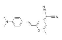
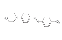
Figure 4: (a) Two-photon emission from a polymer film doped with DCM. A SHG peak appears next to the fluorescence band when a high voltage is applied to the sample (dashed line: 0 V; continuous line: 300 V). (b) SHG modulation from DCM molecules under an ON-OFF poling field. The high background is due to the DCM residual TPF, which lies within the filter bandpass. Note that it would be possible to avoid such a signal by working off resonance for the SHG. (c) Two-photon emission from a polymer film doped with DR1, showing only SHG. The width of the SHG peak is limited by the incoming IR femtosecond laser linewidth. (d) SHG modulation for DR1 molecule. In both cases, the incident IR laser beam energy is about 0.1 nJ per pulse.

The same setup can also be used to study the influence of a non-centrosymmetric contribution of the molecular distribution on the optical response upon two-photon excitation. In this case, a SHG signal arises from the polar orientation of nonlinear active molecules. For this purpose, the DCM doped polymer matrix is spincoated on a set of two transverse electrodes, as described in the first part of this paper. A high voltage of about 300 V, corresponding to a poling field of $3\times 10^{7}$ V.m^-1, is applied by means of electrical contacts on the electrodes. As the DCM molecules have a non negligible permanent dipole moment of about 10 Debye,[23] they will have a tendency to lean towards the electric field direction, thus creating a non-centrosymmetric distribution. Moreover, due to the nonlinear susceptibility $\beta$ of DCM,[23] the molecular orientation can be directly monitored by the onset of a SHG signal in addition to fluorescence as reported in the previous section. In the present configuration, the SHG signal is detected in a reflection configuration. Since the thickness of the molecular layer is much smaller than the coherence length for phase-matching, the molecules can be simply considered as a coherent ensemble of nonlinear radiating dipoles. The SHG signal therefore appears with the same intensity either in the transmitted or in the reflected direction. As shown on Figure 4a, the overall two-photon emission spectrum exhibits a narrow SHG peak at $2\omega$, emerging in the tail of the broadband fluorescence when the electric field is applied. The SHG and TPF signals can be easily selected by introducing appropriate optical filters. Figure 4b shows the temporal evolution of SHG upon the ON-OFF application of the electric field: since the SHG signal disappears when the electric field is turned off, on can assume that the molecules still have a high degree of mobility in the polymer matrix in spite of its high $T_{\textrm{g}}$. This mobility is probably a result of the broad size distribution of cavities in the polymer with a tail in the large size limit.

When spectrally selecting the TPF signal only, the polarization response of the sample does not undergo significant changes in the presence of the static electric field. The fluorescence sensitivity to molecular orientation can be explored by calculating similar polarization patterns as those observed in Figure 2, accounting for the molecular orientational distribution induced by electric field orientation. The calculated fluorescence patterns, shown on Figure 5, have been computed considering a permanent poling field $\vec{E}_{0}$ and using the Boltzmann distribution function:

$$f(\Omega)=\frac{\textrm{e}^{(\vec{\mu}(\Omega).\vec{E}_{0})/k_{B}T)}}{\int\textrm{e}^{(\vec{\mu}(\Omega).\vec{E}_{0})/k_{B}T)}\textrm{d}\Omega}$$ (7)

where $k_{B}$ is the Boltzmann’s constant and $T$ the poling temperature. As seen from Figure 5b in our experimental conditions, i.e. with an electric field of $3\times 10^{7}$ V.m^-1 and at room temperature, the fluorescence patterns exhibit only slight differences compared to an isotropic molecular distribution. This result is not surprising since the TPF intensity is proportional to the number $N$ of active molecules per unit volume, whereas SHG intensity is proportional to $N^{2}$ as a result of the coherence of this radiating process. Moreover, the weak effect of the electric field on the fluorescence anisotropy is also due to the broad statistical orientational Boltzmann distribution at room temperature. Figure 5c shows that orientational effects should be strongly increased with higher electric fields, which are however difficult to reach due to electric breakdown.

Figure 5: Influence of the poling field $\vec{E}_{0}$, aligned along the $X$ axis, on polar polarization plots of the calculated TPF intensities $I_{X}$ (dashed line) and $I_{Y}$ (continuous line) emitted by an assembly of fluorescent molecules. Energy transfer effects are not taken into account in these calculations. All graphs have the same scale (a) Fluorescence diagram for an isotropic molecular distribution. (b) Fluorescence diagram with a field of $3\times 10^{7}$ V.m^-1, such as used in our experiment. There is no clear difference with the first diagram. (c) The effect of the applied field becomes visible for $3\times 10^{8}$ V.m^-1, corresponding to a voltage 10 times higher than the experimentally used values.

The SHG signal is therefore a better suited probe of the field-induced anisotropic molecular distribution.

Figure 6: Polar plots showing the SHG signals (integration time: 100 ms) $I_{X}$ (in dark grey) and $I_{Y}$ (in light grey) emitted by an assembly of DR1 molecules poled under an electric field of $3\times 10^{7}$ V.m^-1 as a function of the incident polarization angle varying from $0^{\circ}$ to $360^{\circ}$. The different diagrams have been obtained for different orientations of the electric field, as indicated on the Figures. (a) and (b): $I_{X}$ and $I_{Y}$ for $\vec{E}_{0}$ along $X$, (c) and (d): $I_{X}$ and $I_{Y}$ for $\vec{E}_{0}$ along $Y$, (e): $I_{X}$ and $I_{Y}$ for $\vec{E}_{0}$ at $45^{\circ}$ of $X$ and $Y$. The continuous lines represent the fit according to the expressions given in Appendix C. The situations where $\vec{E}_{0}$ is along the $X$ or $Y$ axis are symmetric, whereas a rotation of 45^∘ mixes the nonlinear polarization responses together.

In order to retrieve SHG information independently from fluorescence properties, we choose to study more specifically samples doped with the DR1 molecules, so as to prevent from possibly misleading combinations of SHG and TPF signals. This situation is akin to using DCM molecules with non-resonant excitation, where TPF would then be inefficient. DR1 has a non-negligible dipole moment of 8.7 Debye,[24] and a molecular hyperpolarizability $\beta$=289$\times 10^{-40}$ m⁴V^-1 at zero frequency, which amounts to twice that of DCM.[23] Figures 4c and 4d show the effect of electric field poling of DR1 using the same electrode system . The same polarization analysis is applied to investigate the SHG responses, and Figure 6 shows the evolution of the SHG signal with respect to the rotation of the incident polarization $\alpha$.

In order to fit the data, we developed a model elaborating on Ref. [18, 34], based on the macroscopic second order susceptibility $\chi^{(2)}(2\omega;\omega,\omega)$, which is related to the molecular hyperpolarizability $\beta(2\omega;\omega,\omega)$ tensor and the molecular distribution function $f(\Omega)$. Earlier models are extended herein so as to account for specific features pertaining to the two-photon microscopy setup, as detailed in Appendix C. The rod-like DR1 molecule is composed of a conjugated $\pi$ system with an electron acceptor group at one end and a donor group at the other end. The nonlinear susceptibility $\beta$ has therefore only one non-zero component $\beta_{zzz}$, where $z$ defines the molecular axis direction. We denote $\Omega=(\theta,\phi)$ the Euler angles defining $z$ in the macroscopic framework. With $N$ molecules per unit volume, the $\chi^{(2)}$ susceptibility tensor components can be expressed as:

$$\chi_{\scriptscriptstyle{IJK}}^{(2)}=N\beta_{zzz}\int\cos(z,I)\cos(z,J)\cos(z,K)f(\Omega)\textrm{d}\Omega$$ (8)

where the indices $I,J,K=X,Y,Z$ are the coordinates in the macroscopic framework and $f(\Omega)$ is the molecular orientational distribution function given by Eq. (7). The $\cos(z,I)$ functions are the $(\Omega)$ angle dependent projections of the $z$ axis on the $I$ axis. For symmetry reasons, a non-zero value for $\chi^{(2)}$ requires a macroscopic polar order, which is imposed here by the static electric field $\vec{E}_{0}$ applied in the plane of the sample. From the $\chi_{\scriptscriptstyle{IJK}}^{(2)}$ tensor coefficients, we can infer the induced nonlinear polarization $\vec{P}^{(2)}(2\omega)$ defined as:

$$P_{I}^{(2)}(2\omega)=\sum_{J,K}\chi_{\scriptscriptstyle{IJK}}^{(2)}\,E_{J}(\omega)\,E_{K}(\omega)$$ (9)

Note that this expression of $P_{I}^{(2)}(2\omega)$ does not take into account the local field factors $f_{I}^{2\omega}$, $f_{J}^{\omega}$ and $f_{K}^{\omega}$, which is reasonable in the present context of relatively low molecular concentration and weak poling strength.[35] As detailed in Appendix C, this polarization allows us to compute the $2\omega$ radiated field. The correction factors accounting for the collection of light at wide angles are estimated with a model similar to the one used for TPF. Since SHG is a coherent process arising from the induced dipole radiation, the collected field can be written as:

$$\mathcal{E}^{SHG}_{I}(2\omega)=b_{IXX}E_{X}^{2}+b_{IYY}E_{Y}^{2}+b_{IXY}E_{X}E_{Y}$$ (10)

where $b_{IJK}$ are constant coefficients defined in Appendix C. The resulting intensity is proportional to $|\vec{\mathcal{E}}^{SHG}(2\omega)|^{2}$, and the SHG intensities $I_{I}^{\textrm{SHG}}$ detected by the photodiodes after temporal averaging can be finally expressed as:

$$I_{I=X,Y}^{\textrm{SHG}} = b_{IXX}^{2}\,\overline{E_{X}^{4}}+b_{IYY}^{2}\,\overline{E_{Y}^{4}}+(2\,b_{IXX}\,b_{IYY}+b_{IXY}^{2})\,\overline{E_{X}^{2}E_{Y}^{2}}$$ (11)

$$+ 2\,b_{IXX}\,b_{IXY}\,\overline{E_{X}^{3}E_{Y}}+2\,b_{IYY}\,b_{IXY}\,\overline{E_{X}E_{Y}^{3}}$$

Figure 6 represents the experimental data and the theoretical fits for several orientations of the poling field $\vec{E}_{0}$ relative to the ($X,Y$) axes, showing a good agreement. These fits also take into account the ellipticity parameter $\delta=1.15$ rad and the $\gamma$ factor of 0.02 determined previously. Contrary to fluorescence, the low intermolecular distance in the polymer matrix is seen to not affect the polarization response of SHG. These results show that a thorough SHG polarization analysis is able to account for a slight change in molecular organization. In particular, the symmetry features of SHG polarization polar plots shown in Figure 6 are consistent with the rotation of the electric field in the ($X,Y$) plane. Such polarization signatures can be exploited to identify specific molecular orientation directions in the sample plane. In the present case, the $2\omega$ optical response is spatially uniform over a raster scan of 5 $\mu$m$\times$5 $\mu$m (data not shown). This provides clear evidence of the good homogeneity of the field orientation between the two planar electrodes. Such studies are being currently extended to the mapping of molecular polar-orientation in electro-optic devices based on complex electrodes designs,[36] or to lower-scale changes in molecular orientation patterns such as those observed in Langmuir-Blodgett films.[37]

IV. Conclusion

Polarization analysis of the emission response from an assembly of molecules under two-photon excitation contains significant information on their orientational distribution. Focusing on either TPF or SHG furthermore allows one to study either the incoherent, axial even-order processes, or the coherent polar odd-order processes. Combination of these two techniques provides a complete set of informations regarding possible excitation transfer between molecules or orientation of a collection of molecules with very accute sensitivity to the onset of non-centrosymmetric orientational patterns.

The approach presented in this paper can be applied to a broad variety of molecular media, where unknown orientational distribution functions are expressed using spherical harmonics which can be singled-out via their symmetry properties.[22] By taking advantage of the high optical resolution provided by two-photon microscopy, interesting perspectives can be expected in the study of structures involving sub-microscopic scale effects such as in nanocrystals[38, 39] and nanostructured media supporting local field enhancements.[40]

Appendix A: Polarization response of TPF in a high NA microscope setup for wide angle fluorescence collection

The following model is developed for comparison between polarization responses in two perpendicular polarization directions (see Figure 1). In the subsequent derivations, we omit all efficiency parameters that may appear in the intensity expressions, since such parameters are the same for each channel of polarization direction.

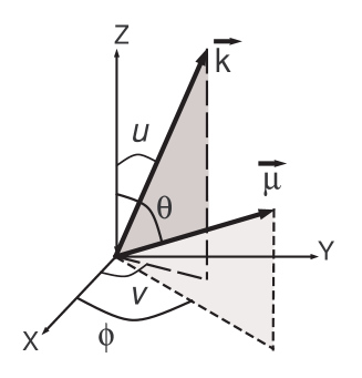
Figure 7: Notations introduced to account for the wide angle collection of the emitted light by a dipole, located at the origin of the $(X,Y,Z)$ framework. The direction of the dipole $\vec{\mu}$ is defined by the angles $(\theta,\phi)$. The direction of the wave vector $\vec{k}$ corresponding to the radiated field, is defined by the angles $(u,v)$.

In order to express the intensity of fluorescence emitted by a single dipole set at the focal point of the microscope objective, we consider the radiation diagram emitted by this dipole $\vec{\mu}$, which orientation is defined by the angles $(\theta,\phi)$, as indicated on Figure 7. The far field radiated in the direction of the wave vector $\vec{k}(u,v)$ is:

$$\vec{\mathcal{E}}^{\textrm{ TPF (radiated)}}\propto\vec{k}\wedge(\vec{\mu}\wedge\vec{k})$$ (12)

were the proportionality factor contains constant radiation field terms that are not used in the following calculations. As the orientation of the wave vector $\vec{k}$ is only defined by the angles ($u,v$), the vector $\vec{\mathcal{E}}^{\textrm{ TPF (radiated)}}$ can be expressed as:

$$\vec{\mathcal{E}}^{\textrm{ TPF (radiated)}}(u,v,\theta,\phi)=\mu_{X}(\theta,\phi)\,\vec{U_{1}}(u,v)+\mu_{Y}(\theta,\phi)\,\vec{U_{2}}(u,v)+\mu_{Z}(\theta,\phi)\vec{U_{3}}(u,v)$$ (13)

where $\vec{U_{1}}$, $\vec{U_{2}}$, $\vec{U_{3}}$ are unit vectors depending only on the parameters $(u,v)$. The field transmitted by the objective can then be expressed as:

$$\vec{\mathcal{E}}^{\textrm{ TPF}}=[\mathcal{R}]\,\vec{\mathcal{E}}^{\textrm{ TPF(radiated)}}$$ (14)

where $[\mathcal{R}]$ represents the rotation matrix simulating the infinity-corrected objective. $[\mathcal{R}]$ is therefore the product of three successive rotations[30] (rotation of $-v$ around $Z$, rotation of $-u$ around $Y$ and rotation of $v$ around $Z$) so as to convert any input incidence on the objective into an output ray parallel to the optical axis $Z$, namely:

$$[\mathcal{R}]=\left[\begin{array}[]{c c c}\cos u\,\cos^{2}v+\sin^{2}v&\cos v\,\sin v(\cos u-1)&-\sin u\,\cos v\\ \cos v\,\sin v(\cos u-1)&\cos u\,\sin^{2}v+\cos^{2}v&-\sin u\,\sin v\\ \sin u\,\cos v&\sin u\,\sin v&\cos u\end{array}\right]$$ (15)

The vector $\vec{\mathcal{E}}^{\textrm{ TPF}}(u,v,\theta,\phi)$ of the trasmitted field can then be expressed as:

$$\mathcal{E}^{\textrm{TPF}}_{X}(u,v,\theta,\phi)=f_{X}(u,v)\,\mu_{X}(\theta,\phi)+f_{Y}(u,v)\,\mu_{Y}(\theta,\phi)+f_{Z}(u,v)\,\mu_{Z}(\theta,\phi)$$

$$\mathcal{E}^{\textrm{TPF}}_{Y}(u,v,\theta,\phi)=g_{X}(u,v)\,\mu_{X}(\theta,\phi)+g_{Y}(u,v)\,\mu_{Y}(\theta,\phi)+g_{Z}(u,v)\,\mu_{Z}(\theta,\phi)$$ (16)

where $f_{X}$, $f_{Y}$, $f_{Z}$, $g_{X}$, $g_{Y}$ and $g_{Z}$ are functions of the $(u,v)$ parameters.

Since fluorescence light is emitted incoherently, the intensities detected by the photodetectors and coming from the single dipole $\vec{\mu}(\theta,\phi)$, are computed after integration of the square of each $\vec{\mathcal{E}}^{\textrm{ TPF}}$ component, over all the angles $(u,v)$ within the half-aperture angle $\theta_{\textrm{obj}}$ of the objective, hence giving the detection probability:

$$J_{I=X,Y}(\theta,\phi)=\int_{0}^{2\pi}\int_{0}^{\theta_{\textrm{obj}}}\big{(}\mathcal{E}^{\textrm{TPF}}_{I}(u,v,\theta,\phi)\big{)}^{2}\sin{u}\,\textrm{d}u\,\textrm{d}v$$ (17)

In the present work, the oil-immersion ($n$=1.5) objective has a numerical aperture NA=1.4. The half-aperture angle $\theta_{\textrm{obj}}$ is therefore equal to $1.204$ rad (69^∘). After integration, the previous expression reduces to:

$$J_{X}(\theta,\phi)=K_{1}\,\mu_{X}^{2}(\theta,\phi)+K_{2}\,\mu_{Y}^{2}(\theta,\phi)+K_{3}\,\mu_{Z}^{2}(\theta,\phi)$$

$$J_{Y}(\theta,\phi)=K_{2}\,\mu_{X}^{2}(\theta,\phi)+K_{1}\,\mu_{Y}^{2}(\theta,\phi)+K_{3}\,\mu_{Z}^{2}(\theta,\phi)$$ (18)

with:

$$K_{1}=\int_{0}^{2\pi}\int_{0}^{\theta_{\textrm{obj}}}f_{X}^{2}(u,v)\sin{u}\,\textrm{d}u\,\textrm{d}v=\int_{0}^{2\pi}\int_{0}^{\theta_{\textrm{obj}}}g_{Y}^{2}(u,v)\sin{u}\,\textrm{d}u\,\textrm{d}v=2.945$$

$$K_{2}=\int_{0}^{2\pi}\int_{0}^{\theta_{\textrm{obj}}}f_{Y}^{2}(u,v)\sin{u}\,\textrm{d}u\,\textrm{d}v=\int_{0}^{2\pi}\int_{0}^{\theta_{\textrm{obj}}}g_{X}^{2}(u,v)\sin{u}\,\textrm{d}u\,\textrm{d}v=0.069$$

$$K_{3}=\int_{0}^{2\pi}\int_{0}^{\theta_{\textrm{obj}}}f_{Z}^{2}(u,v)\sin{u}\,\textrm{d}u\,\textrm{d}v=\int_{0}^{2\pi}\int_{0}^{\theta_{\textrm{obj}}}g_{Z}^{2}(u,v)\sin{u}\,\textrm{d}u\,\textrm{d}v=1.016\,\,$$ (19)

Moreover, the two photon excitation probability, which is proportional to $|\vec{\mu}(\Omega).\vec{E}|^{4}$, can be easily evaluated. Since fluorescence is an incoherent process, we directly integrate the dipole response, product of the excitation and detection probability, over all dipole orientations. Assuming that the absorption and emission dipoles of each chromophore are parallel, the detected intensities can then be expressed as:

$$I_{I=X,Y}^{\textrm{TPF}}=\int\overline{\arrowvert\vec{\mu}(\Omega).\vec{E}\arrowvert^{4}}J_{I}(\Omega)f(\Omega)\textrm{d}\Omega$$ (20)

Developing $\overline{|\vec{\mu}(\Omega).\vec{E}|^{4}}$ in the previous expressions, the TPF intensities, depending only on parameters $(\alpha,\delta,\gamma)$, finally reduce to:

$$I_{I=X,Y}^{\textrm{TPF}}(\alpha,\delta,\gamma) = \sum_{J,K,L,M=X,Y}f_{IJKLM}\,\overline{E_{J}E_{K}E_{L}E_{M}}$$ (21)

$$= f_{IXXXX}\overline{E_{X}^{4}}+f_{IYYYY}\overline{E_{Y}^{4}}+6f_{IXXYY}\overline{E_{X}^{2}E_{Y}^{2}}$$

$$+ 4f_{IXXXY}\overline{E_{X}^{3}E_{Y}}+4f_{IXYYY}\overline{E_{X}E_{Y}^{3}}$$

where the $f_{IJKLM}$ coefficients are defined by:

$$f_{IJKLM}=\int J_{I}(\Omega)\,\mu_{J}(\Omega)\,\mu_{K}(\Omega)\,\mu_{L}(\Omega)\,\mu_{M}(\Omega)\,f(\Omega)\,\textrm{d}\Omega$$ (22)

Appendix B: Expression of the acceptor coordinates $\vec{\mu}_{2}$ in the macroscopic framework

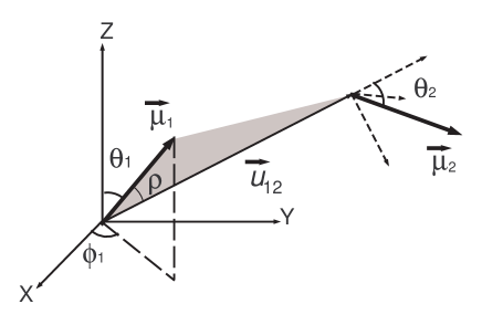
Figure 8: Position and orientation of the acceptor $\vec{\mu}_{2}$ relative to the position and orientation of the donor $\vec{\mu}_{1}$. The orientation of the donor $\vec{\mu}_{1}$ is defined by the ($\theta_{1},\phi_{1}$) angles. The orientation of the unitary vector $\vec{u}_{12}$ along the line connecting the two chromophores is defined by the ($\rho,\xi$) angles in the ($\theta_{1},\phi_{1}$) framework. The orientation of the acceptor $\vec{\mu}_{2}$ in the ($\rho,\xi$) framework is defined by the $(\theta_{2},\phi_{2})$ angles in the local framework of molecule 2 (shown in dotted lines).

As indicated in Figure 8, ($\theta_{1},\phi_{1}$) defines the orientation of the donor dipole $\vec{\mu}_{1}$ and ($\rho,\xi$) defines the orientation of the vector $\vec{u}_{12}$ connecting the two chromophores in the ($\theta_{1},\phi_{1}$) framework. The orientation of the acceptor dipole $\vec{\mu}_{2}$ is defined by the angles $(\theta_{2},\phi_{2})$ in the ($\rho,\xi$) local framework of molecule 2. The acceptor coordinates in the macroscopic framework depend consequently on the angles $(\theta_{2},\phi_{2},\rho,\xi,\theta_{1},\phi_{1})$ and can be written as:

$$\vec{\mu}_{2}(\theta_{2},\phi_{2},\rho,\xi,\theta_{1},\phi_{1})=[\mathcal{M}]_{(\theta_{1},\phi_{1})\to(X,Y,Z)}[\mathcal{M}]_{(\rho,\xi)\to(\theta_{1},\phi_{1})}\left[\begin{array}[]{c}\sin\theta_{2}\cos\phi_{2}\\ \sin\theta_{2}\sin\phi_{2}\\ \cos\theta_{2}\end{array}\right]$$ (26)

where $[\mathcal{M}]_{(\rho,\xi)\to(\theta_{1},\phi_{1})}$ represents the rotation matrix from the $(\rho,\xi)$ framework to the $(\theta_{1},\phi_{1})$ framework and $[\mathcal{M}]_{(\theta_{1},\phi_{1})\to(X,Y,Z)}$ is the rotation matrix from the $(\theta_{1},\phi_{1})$ framework to the macroscopic one. Expressions for these matrices are:

$$[\mathcal{M}]_{(\rho,\xi)\to(\theta_{1},\phi_{1})}=\left[\begin{array}[]{ccc}\sin\rho\cos\xi&\cos\rho\cos\xi&-\sin\xi\\ \sin\rho\sin\xi&\cos\rho\sin\xi&\cos\xi\\ \cos\rho&-\sin\rho&0\\ \end{array}\right]$$ (30)

and:

$$[\mathcal{M}]_{(\theta_{1},\phi_{1})\to(X,Y,Z)}=\left[\begin{array}[]{ccc}\sin\theta_{1}\cos\phi_{1}&\cos\theta_{1}\cos\phi_{1}&-\sin\phi_{1}\\ \sin\theta_{1}\sin\phi_{1}&\cos\theta_{1}\sin\phi_{1}&\cos\phi_{1}\\ \cos\theta_{1}&-\sin\theta_{1}&0\\ \end{array}\right]$$ (34)

The fluorescence intensity emitted by the acceptor can then be expressed as:

$$J_{X}(\Omega_{2},\Omega_{1},\rho,\xi) = K_{1}\,\mu^{2}_{2X}(\theta_{2},\phi_{2},\rho,\xi,\theta_{1},\phi_{1})+K_{2}\,\mu^{2}_{2Y}(\theta_{2},\phi_{2},\rho,\xi,\theta_{1},\phi_{1})$$

$$+ K_{3}\,\mu^{2}_{2Z}(\theta_{2},\phi_{2},\rho,\xi,\theta_{1},\phi_{1})$$

$$J_{Y}(\Omega_{2},\Omega_{1},\rho,\xi) = K_{2}\,\mu^{2}_{2X}(\theta_{2},\phi_{2},\rho,\xi,\theta_{1},\phi_{1})+K_{1}\,\mu^{2}_{2Y}(\theta_{2},\phi_{2},\rho,\xi,\theta_{1},\phi_{1})$$ (35)

$$+ K_{3}\,\mu^{2}_{2Z}(\theta_{2},\phi_{2},\rho,\xi,\theta_{1},\phi_{1})$$

where the parameters $K_{1}$, $K_{2}$ and $K_{3}$ are defined in Appendix A.

Appendix C: Polarization responses of SHG in a high NA microscope setup

In the case of second harmonic generation, the expression of the radiated field is similar to the fluorescence emission, requiring mere replacement of the dipole moment $\vec{\mu}$ by the induced second order nonlinear polarization $\vec{P}^{(2)}$:

$$\vec{\mathcal{E}}^{\textrm{ SHG (radiated)}}(u,v)\propto\vec{k}\wedge(\vec{P}^{(2)}\wedge\vec{k})$$ (36)

with:

$$\vec{P}^{(2)}=\left[\begin{array}[]{c}\chi^{(2)}_{\scriptscriptstyle{XXX}}\\ \chi^{(2)}_{\scriptscriptstyle{YXX}}\\ \chi^{(2)}_{\scriptscriptstyle{ZXX}}\end{array}\right]E_{X}^{2}+\left[\begin{array}[]{c}\chi^{(2)}_{\scriptscriptstyle{XYY}}\\ \chi^{(2)}_{\scriptscriptstyle{YYY}}\\ \chi^{(2)}_{\scriptscriptstyle{ZYY}}\end{array}\right]E_{Y}^{2}+2\left[\begin{array}[]{c}\chi^{(2)}_{\scriptscriptstyle{XXY}}\\ \chi^{(2)}_{\scriptscriptstyle{YXY}}\\ \chi^{(2)}_{\scriptscriptstyle{ZXY}}\end{array}\right]E_{X}E_{Y}$$ (37)

where the $\chi^{(2)}_{\scriptscriptstyle{IJK}}$ coefficients are the tensor coefficients of the macroscopic nonlinear susceptibility $\chi^{(2)}$. The radiated field $\vec{\mathcal{E}}^{\textrm{ SHG(radiated)}}$ is then:

$$\vec{\mathcal{E}}^{\textrm{ SHG(radiated)}}(u,v)=\left[\begin{array}[]{ccc}A_{XXX}&A_{XYY}&A_{XXY}\\ A_{YXX}&A_{YYY}&A_{YXY}\\ A_{ZXX}&A_{ZYY}&A_{ZXY}\end{array}\right]\left[\begin{array}[]{c}E_{X}^{2}\\ E_{Y}^{2}\\ E_{X}E_{Y}\end{array}\right]$$ (38)

where the $A_{IJK}$ coefficients depend only on parameters $(u,v)$. Taking into account the effect of the objective (see Eq. (14)), we can write:

$$\vec{\mathcal{E}}^{\textrm{ SHG}}(u,v)=[\mathcal{R}]\,\vec{\mathcal{E}}^{\textrm{ SHG (radiated)}}=\left[\begin{array}[]{ccc}B_{XXX}&B_{XYY}&B_{XXY}\\ B_{YXX}&B_{YYY}&B_{YXY}\\ B_{ZXX}&B_{ZYY}&B_{ZXY}\end{array}\right]\left[\begin{array}[]{c}E_{X}^{2}\\ E_{Y}^{2}\\ E_{X}E_{Y}\end{array}\right]$$ (39)

where the $B_{IJK}$ coefficients depend only on the $(u,v)$ angles. As SHG signal is emitted through a coherent process, integration over all ($u,v$) angles in the objective aperture is performed before taking the square of the emitted field. The total collected field $\vec{\mathcal{E}}^{\textrm{ SHG}}_{\textrm{tot}}$ is then obtained by integration over the ($u,v$) angular variables:

$$\vec{\mathcal{E}}^{\textrm{ SHG}}_{\textrm{tot}}=\left[\begin{array}[]{ccc}b_{XXX}&b_{XYY}&b_{XXY}\\ b_{YXX}&b_{YYY}&b_{YXY}\\ b_{ZXX}&b_{ZYY}&b_{ZXY}\end{array}\right]\left[\begin{array}[]{c}E_{X}^{2}\\ E_{Y}^{2}\\ E_{X}E_{Y}\end{array}\right]$$ (40)

where:

$$b_{IJK}=\int_{0}^{2\pi}\int_{0}^{\theta_{\textrm{obj}}}B_{IJK}(u,v)\sin u\,\textrm{d}u\,\textrm{d}v$$ (41)

Since the detected intensity is proportional to $\overline{|\vec{\mathcal{E}}^{\textrm{ SHG}}_{\textrm{tot}}|^{2}}$, the expression of $I_{X}$ and $I_{Y}$ are therefore:

$$I_{I=X,Y}^{\textrm{SHG}} = b_{IXX}^{2}\,\overline{E_{X}^{4}}+b_{IYY}^{2}\,\overline{E_{Y}^{4}}+(2\,b_{IXX}\,b_{IYY}+b_{IXY}^{2})\,\overline{E_{X}^{2}E_{Y}^{2}}$$ (42)

$$+ 2\,b_{IXX}\,b_{IXY}\,\overline{E_{X}^{3}E_{Y}}+2\,b_{IYY}\,b_{IXY}\,\overline{E_{X}E_{Y}^{3}}$$

Acknowledgments

The authors are grateful to Christelle Anceau for helpful comments and discussions. They also thank François Treussart and André Clouqueur for technical support and Rolland Hierle for help with the photo-lithographic technique and work facility in the clean-room.

References

- [1] Topics in Fluorescence Spectrosopy; Lakowicz, J. R. Ed.; Plenum Press: New York, USA, 1997; Vol. 5, pp 187-209.
- [2] Denk, W.; Strickler, J. H.; Webb, W. W. Science 1990, 248, 73-76.
- [3] Mertz, J.; Xu, C.; Webb, W. W. Opt. Lett. 1995, 20, 2532-2534.
- [4] Albota, M.; Beljonne, D.; Brédas, J.-L.; Ehrlich, J.E.; Fu, J.-Y.; Heikal, A. A.; Hess S. E.; Kogej, T.; Levin, M. D.; Marder, S. R.; McCord-Maughon, D.; Perry, J. W.; Röckel, H.; Rumi, M.; Subramaniam, G.; Webb, W. W.; Wu, X.-L.; Xu, C. Science 1998, 281, 1653-1656.
- [5] Ventelon, L.; Charier, S.; Moreaux, L.; Mertz, J.; Blanchard-Desce, M.Angew. Chem. Int. Ed. 2001, 40, 2098-2100.
- [6] Barad, Y.; Eisenberg, H.; Horowitz, M.; Silberberg, Y. Appl. Phys. Lett. 1997, 70, 922-925.
- [7] Schins, J. M.; Schrama, T.; Squier, J.; Brakenhoff, G.J.; Müller, M. J. Opt. Soc. Am. B 2002, 19, 1627-1634.
- [8] Jakubczyk, D.; Shen, Y.; Lal, M.; Friend, C.; Kim, K. S.; Świa̧tkiewicz, J.; Prasad, P. N. Opt. Lett. 1999, 24, 1151-1153.
- [9] Bouhelier, A.; Beversluis, M.; Hartschuh, A.; Novotny, L. Phys. Rev. Lett. 2003, 90, 013903-013907.
- [10] Molecular Nonlinear Optics: Materials, Physics and Devices; Zyss, J. Ed.; Academic Press: Boston, USA, 1994; pp 129-209.
- [11] Guyot-Sionnest, P.; Chen, W.; Shen, Y. R. Phys. Rev. B 1986, 33, 8254-8262.
- [12] Salafski, J.S.; Eisenthal, K.B. Chem. Phys. Lett. 2000, 319, 435-439.
- [13] Moreaux, L.; Sandre, O.; Mertz, J. J. Opt. Soc. Am. B 2000, 17, 1685-1694.
- [14] Campagnola, P. J.; Wei, M.; Lewis, A.; Loew, L. M. Biophys. J. 1999, 77, 3341-3349.
- [15] Peleg, G.; Lewis, A.; Linial, M.; Loew, L. M. Proc. Natl. Acad. Sci. USA 1999, 96, 6700-6704.
- [16] Noordman, O.F.J.; Van Hulst, N.F. Chem. Phys. Lett. 1996, 253, 145-150.
- [17] Monson, P. R.; McClain, W. M. J. Chem. Phys. 1970, 53, 29-37.
- [18] van der Vorst, C. P. J. M.; Picken, S. J. J. Opt. Soc. Am. B 1990, 7, 320-325.
- [19] Singer, K. D.; King, L. A. J. Appl. Phys. 1991, 70, 3251-3255.
- [20] Brasselet, S.; Zyss, J. Opt. Lett. 1997, 22, 1464-1466.
- [21] Dumont, M.; El Osman, A. Chem. Phys. 1999, 245, 437-447.
- [22] Brasselet, S.; Bidault, S.; Zyss, J. C.R. Acad. Sci. Phys.(Paris) 2002, 3, 479-489.
- [23] Moylan, C. R.; Ermer, S.; Lovejoy, S. M.; McComb, I.-H.; Leung, D.S.; Wortmann, R.; Krdmer, P.; Twieg, R. J. J. Am. Chem. Soc. 1996, 118, 21950-12955.
- [24] Singer, K. D.; Sohn, J. E.; King, L. A.; Gordon, H. M.; Katz, H. E.; Dirk, C. W. J. Opt. Soc. Am. B 1989, 6, 1339-1350.
- [25] The microscope slides were carefully cleaned with acetone, ethanol and ultra-pure water. We verified that undopped polymer sample did not exhibit any measurable signal under two-photon excitation.
- [26] The wavelength distribution in the femtosecond pulses is neglegted in this model and only one fundamental pulsation is considered.
- [27] Richards, B.; Wolf, E. Proc. R. Soc. London A 1959, 253, 358-379.
- [28] The Gouÿ phase shift factor contribution has been shown to be of crucial importance in the case of SHG transmitted signals with distances along longer than the coherence length of the nonlinear process. In our reflection configuration, the nonlinear interaction takes place in the sample plane and the propagation length is lower than the coherence length, therefore a possible contribution factor does not affect the propagation of the SHG signal. This factor only brings a constant contribution to the SHG polarized signal level, which has been quantified accounting for our 1.4 numerical aperture, and seen to be negligible compared with the other in-plane contributions.
- [29] Mertz, J.; Moreaux, L. Opt. Comm. 2001, 196, 325-330.
- [30] Axelrod, D. Biophys. J. 1979, 26, 557-573.
- [31] The angle between the two dipoles of absorption and emission for DCM has been estimated separately using static fluorescence anisotropy measurements in solution. The measured value is around 25∘, which does not significantly influence the results in the model, compared with the other effects described in this work.
- [32] Penzkofer, A.; Leupacher, W. J. Luminesc. 1987, 37, 61-72.
- [33] Clegg, R. M. In Fluorescence Imaging Spectroscopy and Microscopy; Wang, X. F.; Herman, B., Eds.; Chemical Analysis Series; Wiley: New York, USA, 1996, Vol. 137, pp 179-252.
- [34] Singer, K. D.; Kusyk, M. G.; Sohn, J. E. J. Opt. Soc. Am. B 1987, 4, 968-976.
- [35] Pliska, T.; Cho, W.-R.; Meier, J.; Le Duff, A. C.; Ricci, V.; Otomo, A.; Canva, M.; Stegeman, G. I.; Raimond, P.; Kajzar, F. J. Opt. Soc. Am. B 2000, 17, 1554-1564.
- [36] Donval, A.; Toussaere, E.; Hierle, R.; Zyss, J. J. Appl. Phys. 2000, 87, 3258-3262.
- [37] Bozhevolnyi, S. I.; Geisler, T. J. Opt. Soc. Am. A 1998, 15, 2156-2162.
- [38] Shen, Y.; Markowicz, P.; Winiarz, J.; Swiatkiewicz, J.; Prasad, P. N. Opt. Lett. 2001, 26, 725-727.
- [39] Treussart, F.; Botzung-Appert, E.; Ha-Duong, N.-T.; Ibanez, A.; Roch, J.-F.; Pansu, R. Chem. Phys. Chem. 2003, in press.
- [40] Anceau, C.; Brasselet, S.; Zyss, J.; Gadenne, P. Opt. Lett. 2003, in press.