Crossover behavior in three-dimensional dilute spin systems

Abstract

We study the crossover behaviors that can be observed in the high-temperature phase of three-dimensional dilute spin systems, using a field-theoretical approach. In particular, for randomly dilute Ising systems we consider the Gaussian-to-random and the pure-Ising-to-random crossover, determining the corresponding crossover functions for the magnetic susceptibility and the correlation length. Moreover, for the physically interesting cases of dilute Ising, XY, and Heisenberg systems, we estimate several universal ratios of scaling-correction amplitudes entering the high-temperature Wegner expansion of the magnetic susceptibility, of the correlation length, and of the zero-momentum quartic couplings.

I Introduction.

The critical behavior of randomly dilute magnetic materials is of considerable theoretical and experimental interest [1, 2, 3, 4, 5]. A simple model describing these systems is provided by the Hamiltonian

$${\cal H}_{p}=J\,\sum_{<ij>}\rho_{i}\,\rho_{j}\;s_{i}\cdot s_{j},$$ (1)

where the sum is extended over all nearest-neighbor sites, $s_{i}$ are $M$-component spin variables, and $\rho_{i}$ are uncorrelated quenched random variables, which are equal to one with probability $p$ (the spin concentration) and zero with probability $1-p$ (the impurity concentration). For sufficiently low dilution $1-p$, i.e. above the percolation threshold of the spins, the system described by the Hamiltonian ${\cal H}_{p}$ undergoes a second-order phase transition at $T_{c}(p)<T_{c}(p=1)$.

The nature of the transition is rather well established. In the case of the random Ising model (RIM) corresponding to $M=1$, the transition belongs to a new universality class which is distinct from the Ising universality class describing the critical behavior of the pure system. This has been clearly observed in experiments [3] on dilute uniaxial antiferromagnets, such as Fe_xZn_1-xF₂ and Mn_xZn_1-xF₂, in the absence of magnetic field [6] and in Monte Carlo simulations of the RIM, see, e.g., Refs. [7, 8, 9, 10]. The critical exponents are independent of the impurity concentration and definitely different from those of the pure Ising universality class. Field-theoretical (FT) studies [11, 12, 13, 14, 15, 16] confirm these results. The fixed point (FP) related to the pure Ising universality class is unstable with respect to the addition of impurities and the renormalization-group (RG) flow is driven towards a new stable random FP that controls the critical behavior.

Unlike Ising systems, multicomponent O($M$)-symmetric spin systems do not change their asymptotic critical behavior in the presence of random impurities. Indeed, according to the Harris criterion [17], the addition of impurities to a system which undergoes a continuous transition does not change the critical behavior if the specific-heat critical exponent $\alpha$ of the pure system is negative, as is the case for any $M\geq 2$. From the point of view of RG theory, the Wilson-Fisher FP of the pure O($M$) theory is stable under random dilution. The presence of impurities affects only the approach to the critical regime, giving rise to scaling corrections behaving as $|\tau|^{\Delta_{1}}$, where $\tau$ is the reduced temperature and $\Delta_{1}=-\alpha$. The exponent $\Delta_{1}$ is rather small for the physically relevant cases $M=2$ and $M=3$—$\alpha=-0.0146(8)$ (Ref. [18]) and $\alpha=-0.1336(15)$ (Ref. [19]), respectively—giving rise to very slowly decaying scaling corrections. Experiments on ⁴He in porous materials [20, 21] and on randomly dilute isotropic magnetic materials, see, e.g., Refs. [22, 23, 24], show that the critical exponents of XY and Heisenberg systems are unchanged by disorder (see also the list of results reported in Ref. [4]). But, in order to observe the correct exponents in magnetic systems in which the reduced temperature is usually not smaller than $10^{-3}$, it is important to keep into account the scaling corrections in the analysis of the experimental data [22].

In this paper we study the crossover behaviors that can be observed in the high-temperature phase of three-dimensional dilute spin systems. First, we consider the crossover from the Gaussian FP to the stable FP of the model, i.e. the random FP for $M=1$ and the pure $O(M)$-symmetric FP for $M\geq 2$. Such a crossover can be observed at fixed impurity concentration by varying the temperature. If $|T-T_{c}|/T_{c}>G$, where $G$ is an appropriate Ginzburg number [25], fluctuations are irrelevant and mean-field behavior is expected, while for $|T-T_{c}|/T_{c}<G$ the asymptotic critical behavior sets in. This crossover is not universal. Nonetheless, there are limiting situations in which the crossover functions become independent of the microscopic details of the statistical system: This is the case of the critical crossover limit of systems with medium-range interactions, i.e. of systems in which the interaction scale is larger than the typical microscopic scale [26]. In this limit the crossover functions can be computed by using FT methods: for $O(M)$ models precise results have been obtained in Ref. [27] by using the three-dimensional massive scheme and in Refs. [28, 29] by using the minimal-subtraction scheme without $\epsilon$ expansion.

In Ising systems there is also another interesting crossover associated with the RG flow from the pure Ising FP to the random FP. When the concentration $p$ is close to 1, by decreasing the temperature at fixed $p$, one first observes Ising critical behavior, then a crossover sets in, ending with the expected random critical behavior. In a suitable limit in which $p\to 1$ this crossover is universal. The corresponding universal crossover functions can be computed by using FT methods.

These crossover behaviors are investigated here by using the fixed-dimension perturbative approach in powers of appropriate zero-momentum quartic couplings. We determine the RG trajectories and the crossover functions of the magnetic susceptibility $\chi$ and of the second-moment correlation length $\xi$, defined from the two-point function

$$G(x)\equiv\overline{\langle\rho_{0}\,\rho_{x}\;s_{0}\cdot s_{x}\rangle},$$ (2)

where the overline indicates the average over dilution and $\langle\;\;\rangle$ indicates the sample average at fixed disorder. This study allows us to compute the corresponding effective exponents and to determine several universal ratios of scaling-correction amplitudes entering their high-temperature Wegner expansions. Beside $\chi$ and $\xi$, we also consider zero-momentum quartic correlations and appropriate combinations that have a universal high-temperature critical limit, such as

$$G_{4} \equiv -{3M\over M+2}\lim_{\tau\to 0^{+}}{\chi_{4}\over\xi^{3}\chi^{2}},$$ (3)

$$G_{22} \equiv -\lim_{\tau\to 0^{+}}{\chi_{22}\over\xi^{3}\chi^{2}},$$ (4)

where $\tau$ is the reduced temperature, $\chi_{4}$ is the zero-momentum four-point connected correlation function averaged over dilution, i.e., setting $\mu\equiv\sum_{x}\rho_{x}s_{x}$,

$$V\chi_{4}=\overline{\langle(\mu\cdot\mu)^{2}\rangle-\frac{M+2}{M}\,\langle\mu\cdot\mu\rangle^{2}},$$ (5)

and $\chi_{22}$ is defined by

$$V\chi_{22}=\overline{\langle\mu\cdot\mu\rangle^{2}}-\overline{\langle\mu\cdot\mu\rangle}^{2}.$$ (6)

Their high-temperature Wegner expansion is given by

$$\chi=\chi_{\tau}\tau^{\,-\gamma}\left(1+\chi_{\tau,1}\tau^{\,\Delta_{1}}+\chi_{\tau,2}\tau^{\,\Delta_{2}}+...\right),$$ (7)

$$\xi=\xi_{\tau}\tau^{\,-\nu}\left(1+\xi_{\tau,1}\tau^{\,\Delta_{1}}+\xi_{\tau,2}\tau^{\,\Delta_{2}}+...\right),$$ (8)

$$G_{\#}=G_{\#}^{*}\left(1+G_{\#,\tau,1}\tau^{\,\Delta_{1}}+G_{\#,\tau,2}\tau^{\,\Delta_{2}}+...\right),$$ (9)

where $\Delta_{1,2}$ are the exponents associated with the first two independent scaling corrections. For dilute Ising systems, a recent Monte Carlo study [8] provided the estimate $\Delta_{1}=0.25(3)$; a rough estimate of $\Delta_{2}$ is $\Delta_{2}=0.55(15)$, cf. Sec. III B. For XY and Heisenberg systems $\Delta_{1}=-\alpha$, while $\Delta_{2}$ coincides with the leading correction-to-scaling exponent of the pure model, $\Delta_{2}=0.53(1)$ for $M=2$ and $\Delta_{2}=0.56(2)$ for $M=3$, cf. Ref. [4]. The ratios $\xi_{\tau,i}/\chi_{\tau,i}$ and $\chi_{\tau,i}/G_{\#,\tau,i}$ for $i=1,2$ are universal. Their determination may be useful for the analysis of experimental or Monte Carlo data. In Eqs. (7–9) we only report the leading term for each correction-to-scaling exponent, but it should be noted that there are also corrections proportional to $\tau^{2\Delta_{1}}$, $\tau^{3\Delta_{1}}$, etc., that may be more relevant—this is the case of systems with $M\geq 2$—than those with exponent $\tau^{\Delta_{2}}$.

The crossover behavior in dilute models was already studied in Refs. [30, 14] in the Ising-like case and in Ref. [31] for multicomponent systems. However, Refs. [30, 14, 31] studied the crossover and computed the related effective exponents with respect to the RG flow parameter, while we compute effective exponents with respect to the reduced temperature, which have a direct physical interpretation.

The paper is organized as follows. In Sec. II we discuss the FT approach. We first introduce the effective Landau-Ginzburg-Wilson $\phi^{4}$ Hamiltonian and some general definitions. Then, we generalize the approach of Ref. [27] by showing how to compute the crossover functions of the magnetic susceptibility and of the correlation length in terms of an effective temperature. These exact expressions allow us to determine the temperature dependence of several quantities near the critical point and, as a consequence, to compute some universal ratios of scaling-correction amplitudes entering the high-temperature Wegner expansion of $\chi$, $\xi$, $G_{4}$, and $G_{22}$ for dilute Ising, XY, and Heisenberg systems. These results are presented in Sec. III. Finally, in Sec. IV we extend the computation to the whole crossover regime, determining RG trajectories and effective exponents for Ising, XY, and Heisenberg systems with random dilution. In the case of Ising systems, we also discuss the Ising-to-RIM crossover, give analytic expressions for the crossover scaling functions—details are reported in App. B—and explicitly compute the crossover function associated with the magnetic susceptibility. In App. A we prove some useful identities among the RG functions introduced in the FT approach.

II RG trajectories and crossover functions

A Definitions

The FT approach is based on an effective Landau-Ginzburg-Wilson Hamiltonian that can be obtained by using the replica method [32, 33, 34, 35], i.e.

$${\cal H}_{MN}=\int d^{d}x\left\{\sum_{ia}{1\over 2}\left[(\partial_{\mu}\phi_{ai})^{2}+r\phi_{ai}^{2}\right]+\sum_{ijab}{1\over 4!}\left(u_{0}+v_{0}\delta_{ij}\right)\phi^{2}_{ai}\phi^{2}_{bj}\right\},$$ (10)

where $a,b=1,...M$ and $i,j=1,...N$. In the limit $N\rightarrow 0$ the Hamiltonian ${\cal H}_{MN}$ with $u_{0}<0$ and $v_{0}>0$ is expected to describe the critical properties of dilute $M$-component spin systems. Thus, their critical behavior can be investigated by studying the RG flow of ${\cal H}_{MN}$ in the limit $N\rightarrow 0$. For generic values of $M$ and $N$, the Hamiltonian ${\cal H}_{MN}$ describes $M$ coupled $N$-vector models and it is usually called $MN$ model [1]. ${\cal H}_{MN}$ is bounded from below for $Nu_{0}+v_{0}>0$ and $u_{0}+v_{0}>0$. But, as discussed in Ref. [36], in the limit $N\rightarrow 0$ the only stability condition is $v_{0}>0$. Figure 1 sketches the expected flow diagram in the quartic-coupling plane, for Ising ($M=1$) and multicomponent ($M\geq 2$) systems in the limit $N\rightarrow 0$. The relevant region for dilute systems corresponds to $u<0$ and thus the relevant stable FP is the random FP (RIM in Fig. 1) for $M=1$ and the O($M$) FP for $M\geq 2$.

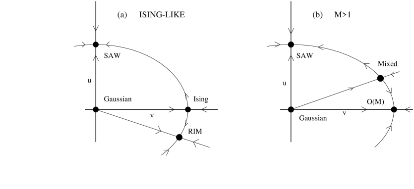
FIG. 1.: Sketch of the RG flow in the coupling plane $(u,v)$ for (a) Ising ($M=1$) and (b) $M$-component ($M>1$) randomly dilute systems.

The most precise FT results have been obtained in the framework of the fixed-dimension expansion in powers of zero-momentum quartic couplings. In this scheme the theory is renormalized by introducing a set of zero-momentum conditions for the one-particle irreducible two-point and four-point correlation functions:

$$\Gamma^{(2)}_{ai,bj}(p)=\delta_{ai,bj}Z_{\phi}^{-1}\left[m^{2}+p^{2}+O(p^{4})\right],$$ (11)

where $\delta_{ai,bj}\equiv\delta_{ab}\delta_{ij}$, and

$$\Gamma^{(4)}_{ai,bj,ck,dl}(0)=Z_{\phi}^{-2}m\left(uS_{ai,bj,ck,dl}+vC_{ai,bj,ck,dl}\right),$$ (12)

where

$$S_{ai,bj,ck,dl} = {1\over 3}\left(\delta_{ai,bj}\delta_{ck,dl}+\delta_{ai,ck}\delta_{bj,dl}+\delta_{ai,dl}\delta_{bj,ck}\right),$$ (13)

$$C_{ai,bj,ck,dl} = {1\over 3}\,\delta_{ij}\delta_{ik}\delta_{il}\,\left(\delta_{ab}\delta_{cd}+\delta_{ac}\delta_{bd}+\delta_{ad}\delta_{bc}\right).$$ (14)

In addition one defines the function $Z_{t}$ through the relation

$$\Gamma^{(1,2)}_{ai,bj}(0)=\delta_{ai,bj}Z_{t}^{-1},$$ (15)

where $\Gamma^{(1,2)}$ is the one-particle irreducible two-point function with an insertion of $\frac{1}{2}\sum_{ai}\phi_{ai}^{2}$.

The critical behavior is determined by the stable FP of the theory, i.e. by the common zero $u^{*}$, $v^{*}$ of the $\beta$-functions

$$\beta_{u}(u,v)=\left.m{\partial u\over\partial m}\right|_{u_{0},v_{0}},\qquad\beta_{v}(u,v)=\left.m{\partial v\over\partial m}\right|_{u_{0},v_{0}},$$ (16)

whose stability matrix has positive eigenvalues (actually a positive real part is sufficient). The critical exponents are obtained by evaluating the RG functions

$$\eta_{\phi}(u,v)={\partial\ln Z_{\phi}\over\partial\ln m},\qquad\eta_{t}(u,v)={\partial\ln Z_{t}\over\partial\ln m}$$ (17)

at $u^{*},v^{*}$:

$$\eta=\eta_{\phi}(u^{*},v^{*}),\qquad{1\over\nu}=2-\eta_{\phi}(u^{*},v^{*})+\eta_{t}(u^{*},v^{*}).$$ (18)

The six-loop pertubative expansions of the $\beta$ functions and of the critical exponents are reported in Refs. [11, 37].

In the $MN$ model, the RG functions satisfy a number of identities. Along the $u=0$ axis we have

$$\left.{\partial\beta_{u}\over\partial u}\right|_{u=0}-\left.{\partial\beta_{v}\over\partial v}\right|_{u=0}+\left.{\partial\beta_{v}\over\partial u}\right|_{u=0}=0,$$ (19)

$$\left.{\partial\eta_{\phi}\over\partial u}\right|_{u=0}-\left.{\partial\eta_{\phi}\over\partial v}\right|_{u=0}=0,$$ (20)

while along the $v=0$ axis we obtain

$$\left.{\partial\beta_{u}\over\partial u}\right|_{v=0}-\left.{\partial\beta_{v}\over\partial v}\right|_{v=0}-{MN+2\over M+2}\,\left.{\partial\beta_{u}\over\partial v}\right|_{v=0}=0,$$ (21)

$$\left.{\partial\eta_{\phi}\over\partial u}\right|_{v=0}-{MN+2\over M+2}\,\left.{\partial\eta_{\phi}\over\partial v}\right|_{v=0}=0,$$ (22)

$$\left.{\partial\eta_{t}\over\partial u}\right|_{v=0}-{MN+2\over M+2}\,\left.{\partial\eta_{t}\over\partial v}\right|_{v=0}=0.$$ (23)

These identities can be proved order by order in the pertubative expansion, see App. A. The second set of relations was already reported in Ref. [38] for $M=1$.

In the limit $N\rightarrow 0$, the perturbative expansions in powers of $u$ and $v$ are not Borel summable at fixed ratio $u/v$ (Ref. [39] shows it explicitly for the zero-dimensional theory with $M=1$, but the argument has general validity), except when $u=0$ that corresponds to the O($M$)-symmetric $\phi^{4}$ theory. For $M\geq 2$, this is a minor problem since the relevant FP is the O($M$)-symmetric one. On the other hand, this is a notable limitation of the perturbative approach for the RIM. Nevertheless, rather reliable results for the critical exponents of the RIM universality class have been obtained from the analysis of properly resummed perturbative series. Several methods have been used: the Padé-Borel method at fixed $u/v$ or the strictly related Chisholm-Borel method, the direct conformal-mapping method, an expansion around the Ising FP [7], the double-Padé-Borel and the conformal-Padé-Borel method [11], which, at least in zero dimensions [40], are able to treat correctly the non-Borel summability of the expansions at fixed $u/v$. The FT estimates of the critical exponents obtained from the analysis of the six-loop expansions reported in Refs. [37, 11] depend only slightly on the resummation method. For instance, Ref. [11] reports $\nu=0.673(8)$ and $\eta=0.029(3)$ from the direct conformal-mapping method, and $\nu=0.678(10)$ and $\eta=0.030(3)$ from an analysis that follows the ideas of Ref. [40]. A second source of uncertainty is the position of the FP. Monte Carlo [7] simulations give $u^{*}=-18.6(3)$ and $v^{*}=43.3(2)$, which are significantly different from the FT estimates [11] $u^{*}=-13(2)$ and $v^{*}=38.0(1.5)$, obtained from the numerical determination of the stable common zero of the $\beta$-functions. However, as discussed in Ref. [7], the critical-exponent estimates show a relatively small dependence on the position of the FP. By using the Monte Carlo results for the location of the FP in the $u$-$v$ plane, one obtains [7] $\nu=0.686(4)$ and $\eta=0.026(3)$, which are close to the above-reported ones, obtained by using the field-theoretical estimates of the FP. In any case, it is reassuring that the FT results are in satisfactory agreement with the Monte Carlo estimates of the critical exponents, i.e. [7] $\nu=0.683(3)$ and $\eta=0.035(2)$. The comparison of the different analyses shows that all different resummation methods give results of similar accuracy. In particular, the more sophisticated analyses suggested in Ref. [40] and employed in Ref. [11] apparently do not provide more accurate results than those at fixed $u/v$. For this reason, in the following we only use the Padé-Borel and the conformal-mapping method at fixed $u/v$. In the latter case, for the singularity of the Borel transform we use the naive analytic continuation for $N\to 0$ of the result for the cubic model reported in Ref. [37]. The results of Ref. [39] suggest that this should allow us to take into account the leading divergent behavior of the series at least for sufficiently small $|u/v|$ (in zero dimensions for $-1/2<u/v<0$).

B Renormalization-group trajectories

The RG trajectories in the plane $(u,v)$ are lines which start from the Gaussian FP located at $u=v=0$ and along which the quartic Hamiltonian parameters $u_{0}$ and $v_{0}$ are kept fixed. They are implicitly characterized by the equation

$$F(u,v)\equiv{uZ_{u}(u,v)\over vZ_{v}(u,v)}={u_{0}\over v_{0}}\equiv s.$$ (24)

RG trajectories can also be determined by solving the differential equations

$$-\lambda{du\over d\lambda}=\beta_{u}(u(\lambda),v(\lambda)),$$ (25)

$$-\lambda{dv\over d\lambda}=\beta_{v}(u(\lambda),v(\lambda)),$$ (26)

where $\lambda\in[0,\infty)$, with the initial conditions

$$u(0)=v(0)=0,$$ (27)

$$\left.{du\over d\lambda}\right|_{\lambda=0}=s,\qquad\left.{dv\over d\lambda}\right|_{\lambda=0}=1.$$ (28)

The solutions $u(\lambda,s)$ and $v(\lambda,s)$ provide the RG trajectories in the $(u,v)$ plane as a function of $s$. The RG trajectories relevant for dilute spin systems are those with $s<0$. The attraction domain of the stable FP is given by the values of $u_{0}$ and $v_{0}$ corresponding to trajectories ending at the stable FP, i.e. trajectories for which

$$u(\lambda=\infty,s)=u^{*},\qquad v(\lambda=\infty,s)=v^{*}.$$ (29)

The crossover functions from the Gaussian to the Wilson-Fisher stable FP have been much studied in the case of the O($M$)-symmetric theories, both in the field theory [27, 28, 29] and in medium-range models [26]. In order to determine the crossover functions along the RG trajectories, and in particular those related with the correlation length $\xi$, the magnetic susceptibility $\chi$, and the reduced temperature $\tau\propto r-r_{c}$, we extend the method of Ref. [27] to Hamiltonians with many quartic parameters, such as ${\cal H}_{MN}$. Using the relations

$$\xi=1/m,\qquad\overline{\chi}\equiv{1\over M}\chi=Z_{\phi}\xi^{2},$$ (30)

$$\Gamma^{(1,2)}_{ai,bj}(0)=\left.{\partial\Gamma^{(2)}_{ai,bj}(0)\over\partial\tau}\right|_{u_{0},v_{0}}=\delta_{ai,bj}\left.{\partial\overline{\chi}^{\,-1}\over\partial\tau}\right|_{u_{0},v_{0}}=\delta_{ai,bj}Z_{t}^{-1},$$ (31)

and Eq. (17), and defining

$$\hat{\eta}_{\phi}(\lambda,s)\equiv\eta_{\phi}(u(\lambda,s),v(\lambda,s)),$$ (32)

$$\hat{\eta}_{t}(\lambda,s)\equiv\eta_{t}(u(\lambda,s),v(\lambda,s))-\eta_{\phi}(u(\lambda,s),v(\lambda,s)),$$ (33)

we derive the following expressions

$$\widetilde{\xi}(\lambda,s)\equiv\xi v_{0}=\lambda,$$ (34)

$$\widetilde{\chi}(\lambda,s)\equiv\overline{\chi}v_{0}^{2}=\lambda^{2}\exp\left[-\int_{0}^{\lambda}dx\,{\hat{\eta}_{\phi}(x,s)\over x}\right],$$ (35)

$$\widetilde{\tau}(\lambda,s)=\tau/v_{0}^{2}=\int_{\lambda}^{\infty}dx\,{2-\hat{\eta}_{\phi}(x,s)\over x^{3}}\,\exp\int_{0}^{x}dy{\hat{\eta}_{t}(y,s)\over y},$$ (36)

where $\widetilde{\xi}$, $\widetilde{\chi}$, and $\widetilde{\tau}$ are dimensionless quantities. One can easily verify that in the Gaussian limit, i.e. for $\lambda\rightarrow 0^{+}$ or $\widetilde{\tau}\rightarrow\infty$, we have $u,v=O(\lambda)$, $\hat{\eta}_{\phi}(\lambda,s)=O(\lambda^{2})$, $\hat{\eta}_{t}(\lambda,s)=O(\lambda)$; therefore $\widetilde{\tau}\widetilde{\xi}^{\,2}\rightarrow 1$ and $\widetilde{\chi}\widetilde{\xi}^{\,-2}\rightarrow 1$, as expected.

Eqs. (34–36) allow us to compute $\widetilde{\xi}$ and $\widetilde{\chi}$ as functions of $\widetilde{\tau}$ and $s$. We can then define effective exponents by taking logarithmic derivatives of $\widetilde{\xi}$ and $\widetilde{\chi}$ at fixed $s$:

$$\nu_{\rm eff}(\widetilde{\tau},s)\equiv-\left.{\partial{\rm ln}\widetilde{\xi}\over\partial{\rm ln}\widetilde{\tau}}\right|_{s},\qquad\gamma_{\rm eff}(\widetilde{\tau},s)\equiv-\left.{\partial{\rm ln}\widetilde{\chi}\over\partial{\rm ln}\widetilde{\tau}}\right|_{s},\qquad\eta_{\rm eff}(\widetilde{\tau},s)\equiv 2-\left.{\partial{\rm ln}\widetilde{\chi}\over\partial{\rm ln}\widetilde{\xi}}\right|_{s}.$$ (37)

One can easily check that $\eta_{\rm eff}=2-\gamma_{\rm eff}/\nu_{\rm eff}=\hat{\eta}_{\phi}$. On the other hand, $\gamma_{\rm eff}\not=\gamma(u,v)$ and $\nu_{\rm eff}\not=\nu(u,v)$ where $\gamma(u,v)$ and $\nu(u,v)$ are the RG functions associated with the exponents $\gamma$ and $\nu$.

III Universal ratios of scaling-correction amplitudes

A General results

In order to determine the scaling-correction amplitudes, we compute the crossover functions close to the critical point, i.e., for $\lambda\rightarrow\infty$ or $\widetilde{\tau}\rightarrow 0^{+}$. For this purpose, we consider the expansion of the RG functions around the stable FP $(u^{*},v^{*})$. We write

$$\beta_{u}(u,v)\approx b_{uu}(u-u^{*})+b_{uv}(v-v^{*}),$$ (38)

$$\beta_{v}(u,v)\approx b_{vu}(u-u^{*})+b_{vv}(v-v^{*}).$$ (39)

Then, using Eq. (26) we have the following behavior, in the limit $\lambda\rightarrow\infty$ and for values of $s$ in the attraction domain of the stable FP,

$$u(\lambda,s)\approx u^{*}+u_{\lambda,1}(s)\lambda^{-\omega_{1}}+u_{\lambda,2}(s)\lambda^{-\omega_{2}}+...,$$ (40)

$$v(\lambda,s)\approx v^{*}+v_{\lambda,1}(s)\lambda^{-\omega_{1}}+v_{\lambda,2}(s)\lambda^{-\omega_{2}}+...,$$ (41)

where $\omega_{1},\omega_{2}$ are the eigenvalues of the matrix

$$\left(\matrix{b_{uu}&b_{uv}\cr b_{vu}&b_{vv}}\right),$$ (42)

and we are keeping only the leading terms in powers of $\lambda^{-\omega_{1}}$ and $\lambda^{-\omega_{2}}$. In particular, we have neglected terms of order $\lambda^{-2\omega_{1}}$, $\lambda^{-3\omega_{1}}$, etc., which may be as important as those of order $\lambda^{-\omega_{2}}$. Moreover, we have

$$R_{1}\equiv{u_{\lambda,1}(s)\over v_{\lambda,1}(s)}={\omega_{1}-b_{vv}\over b_{vu}}={b_{uv}\over\omega_{1}-b_{uu}},$$ (43)

$$R_{2}\equiv{u_{\lambda,2}(s)\over v_{\lambda,2}(s)}={\omega_{2}-b_{vv}\over b_{vu}}={b_{uv}\over\omega_{2}-b_{uu}}.$$ (44)

These ratios are independent of $s$, as expected because they are universal. Indeed, as we shall see, they can be related to the universal ratios $G_{22,\tau,i}/G_{4,\tau,i}$ of the scaling-correction amplitudes of $G_{4}$ and $G_{22}$, cf. Eqs. (4) and (9).

We also expand the RG functions associated with the critical exponents,

$$\nu(u,v)\equiv{1\over 2+\eta_{t}(u,v)-\eta_{\phi}(u,v)}\approx\nu+\nu_{u}(u-u^{*})+\nu_{v}(v-v^{*}),$$ (45)

$$\gamma(u,v)\equiv\left[2-\eta_{\phi}(u,v)\right]\nu(u,v)\approx\gamma+\gamma_{u}(u-u^{*})+\gamma_{v}(v-v^{*}).$$ (46)

and define the $s$-independent quantities

$$\gamma_{\lambda,i}\equiv\gamma_{u}R_{i}+\gamma_{v},\qquad\nu_{\lambda,i}\equiv\nu_{u}R_{i}+\nu_{v},\qquad\Delta_{i}=\omega_{i}\nu,$$ (47)

for $i=1,2$. Then, using Eq. (41), we find

$$\widetilde{\chi}(\lambda,s)=\chi_{\lambda}(s)\lambda^{2-\eta}\left(1+\sum_{i=1}^{2}\chi_{\lambda,i}(s)\lambda^{-\omega_{i}}+...\right),$$ (48)

$$\chi_{\lambda}(s)=\exp\left(-\int_{0}^{1}dx\;{\hat{\eta}_{\phi}(x,s)\over x}-\int_{1}^{\infty}dx\;{\hat{\eta}_{\phi}(x,s)-\eta\over x}\right),$$ (49)

$$\chi_{\lambda,i}(s)={\gamma\over\Delta_{i}}\left({\nu_{\lambda,i}\over\nu}-{\gamma_{\lambda,i}\over\gamma}\right)v_{\lambda,i}(s),$$ (50)

and

$$\widetilde{\tau}(\lambda,s)=\tau_{\lambda}(s)\lambda^{-1/\nu}\left(1+\sum_{i=1}^{2}\tau_{\lambda,i}(s)\lambda^{-\omega_{i}}+...\right),$$ (51)

$$\tau_{\lambda}(s)=\gamma\exp\left(-\int_{0}^{1}dx\;{\hat{\eta}_{t}(x,s)\over x}-\int_{1}^{\infty}dx\;{\hat{\eta}_{t}(x,s)+2-1/\nu\over x}\right),$$ (52)

$$\tau_{\lambda,i}(s)=\left({\gamma_{\lambda,i}\over(1+\Delta_{i})\gamma}-{\nu_{\lambda,i}\over\Delta_{i}\nu}\right)v_{\lambda,i}(s).$$ (53)

Using Eqs. (50) and (53), we can derive the Wegner expansion of $\xi$, $\chi$, and of the zero-momentum quartic couplings $u$ and $v$ in terms of the reduced temperature $\widetilde{\tau}$. We obtain

$$\widetilde{\xi}(\widetilde{\tau},s)=\xi_{\tau}(s)\widetilde{\tau}^{\,-\nu}\left(1+\sum_{i=1}^{2}\xi_{\tau,i}(s)\widetilde{\tau}^{\,\Delta_{i}}+...\right),$$ (54)

$$\xi_{\tau}(s)=\tau_{\lambda}(s)^{\nu},\qquad\xi_{\tau,i}(s)=\nu\tau_{\lambda,i}(s)\,v_{\lambda,i}(s)\,\tau_{\lambda}(s)^{-\Delta_{i}},$$ (55)

and

$$\widetilde{\chi}(\widetilde{\tau},s)=\chi_{\tau}(s)\widetilde{\tau}^{\,-\gamma}\left(1+\sum_{i=1}^{2}\chi_{\tau,i}(s)\widetilde{\tau}^{\,\Delta_{i}}+...\right),$$ (56)

$$\chi_{\tau}(s)=\chi_{\lambda}(s)\tau_{\lambda}(s)^{\gamma},\qquad\chi_{\tau,i}(s)=-{\gamma_{\lambda,i}\over\Delta_{i}(1+\Delta_{i})}v_{\lambda,i}(s)\tau_{\lambda}(s)^{-\Delta_{i}},$$ (57)

and also

$$v(\widetilde{\tau},s)=v^{*}+\sum_{i=1}^{2}v_{\tau,i}(s)\widetilde{\tau}^{\,\Delta_{i}}+...,\qquad v_{\tau,i}(s)=v_{\lambda,i}(s)\,\tau_{\lambda}(s)^{-\Delta_{i}},$$ (58)

$$u(\widetilde{\tau},s)=u^{*}+\sum_{i=1}^{2}u_{\tau,i}(s)\widetilde{\tau}^{\,\Delta_{i}}+...,\qquad u_{\tau,i}(s)=R_{i}\,v_{\lambda,i}(s)\,\tau_{\lambda}(s)^{-\Delta_{i}}.$$ (59)

The results of Ref. [41] allow us to identify

$$G_{4}(\widetilde{\tau},s)=v(\widetilde{\tau},s),\qquad G_{22}(\widetilde{\tau},s)={1\over 3}u(\widetilde{\tau},s),$$ (60)

and to obtain the corresponding scaling-correction amplitudes $G_{4,\tau,i}$ and $G_{22,\tau,i}$ defined in Eq. (9).

From the above-reported relations we derive the following expressions for the universal ratios of scaling-correction amplitudes

$${u_{\tau,i}\over v_{\tau,i}}=R_{i},$$ (61)

$${\xi_{\tau,i}\over\chi_{\tau,i}}={\nu_{\lambda,i}(1+\Delta_{i})\over\gamma_{\lambda,i}}-{\nu\Delta_{i}\over\gamma},$$ (62)

$${\chi_{\tau,i}\over v_{\tau,i}}=-{\gamma_{\lambda,i}\over\Delta_{i}(1+\Delta_{i})}.$$ (63)

Their universality is explicitly verified since they are independent of $s\equiv u_{0}/v_{0}$.

B Results for dilute Ising systems

Using the results reported in Sec. III A, we can estimate several universal scaling-correction amplitude ratios. We analyze appropriate perturbative series that can be derived from those of the $\beta$ functions and the critical exponents. Again, we use the conformal-mapping method and the Padé-Borel method at fixed ratio $u/v$. The errors we report take into account the resummation error and the uncertainty in the location of the FP. We compute each quantity at the FT and at the Monte Carlo FP. The final error is such to include both estimates.

As a first step in the analysis we computed the subleading exponents and the ratios $R_{1}$ and $R_{2}$. The exponent $\omega_{1}$ was already computed in Ref. [11], obtaining $\omega_{1}=0.25(10)$ (using the double-Padé-Borel and the conformal-Padé-Borel method) and $\omega_{1}=0.34(11)$ (using the direct conformal-mapping method), in substantial agreement with the Monte Carlo result $\omega_{1}=0.37(5)$ of Ref. [8]. In those analyses the field-theoretical estimates of the FP was used. We tried to compute $\omega_{1}$ by also using the Monte Carlo estimate of the FP. However, all methods gave largely fluctuating results and no estimate could be obtained. Then, we determined $\omega_{2}$. In this case, the conformal-mapping method provided reasonably stable results up to the Monte Carlo FP. We obtained [42] $\omega_{2}=0.8(2)$.

Similar analyses were done for $R_{1}$ and $R_{2}$. Our final results are

$$R_{1}=-0.90(2),\qquad R_{2}=-0.7(3).$$ (64)

Finally, we determined the ratios of scaling-correction amplitudes using relations (63). In order to have a check of the results, for each quantity we considered several series with the same FP value. We obtained

$$\chi_{\tau,1}/\xi_{\tau,1}=1.99(4),$$ (65)

$$\chi_{\tau,1}/G_{4,\tau,1}=-1.0(3),$$ (66)

$$G_{22,\tau,1}/G_{4,\tau,1}=2.1(1),$$ (67)

$$\chi_{\tau,2}/\xi_{\tau,2}=1.7(2),$$ (68)

$$\chi_{\tau,2}/G_{4,\tau,2}=-0.4(2),$$ (69)

$$G_{22,\tau,2}/G_{4,\tau,2}=1.6(7).$$ (70)

The errors take into account the results obtained from different series and different resummation methods, and also the uncertainty on the location of the FP. It is interesting to note that the results for the ratios $\chi_{\tau,i}/\xi_{\tau,i}$ show that the quantity $\chi/\xi^{2}$ has much smaller scaling corrections than $\chi$ and $\xi$. This fact was used in Ref. [7] in order to obtain a precise Monte Carlo estimate of $\eta$ from the high-temperature behavior of $\chi/\xi^{2}$. For comparison, we report the corresponding values for the pure Ising universality class. From the analysis of high-temperature series one obtains $\chi_{\tau,1}/\xi_{\tau,1}=1.11(12)$ (Ref. [43]) and $\chi_{\tau,1}/\xi_{\tau,1}=1.32(10)$ (Ref. [44]), while field theory gives [27] $\chi_{\tau,1}/\xi_{\tau,1}=1.47(4)$ and $\chi_{\tau,1}/G_{4,\tau,1}=-0.30(4)$.

C Results for dilute multicomponent systems

As in the Ising case, we determine the universal ratios of scaling-correction amplitudes by analyzing the six-loop expansions of the $MN$ model [11]. Since the corresponding RG functions must be evaluated at the O($M$)-symmetric FP, i.e. along the $u=0$ axis, the series are Borel summable and the standard conformal-mapping method works well.

Identity (19) allows us to obtain the following exact results for the universal quantities $R_{i}$:

$$R_{1}=-1,\qquad R_{2}=0,$$ (71)

which hold independently of $M$. We also obtain

$$\chi_{\tau,1}/\xi_{\tau,1}=1.97(2),$$ (72)

$$\chi_{\tau,1}/G_{4,\tau,1}=-17(2),$$ (73)

for dilute XY systems, and

$$\chi_{\tau,1}/\xi_{\tau,1}=1.97(2),$$ (74)

$$\chi_{\tau,1}/G_{4,\tau,1}=-2.5(4),$$ (75)

for dilute Heisenberg systems. The ratios $\chi_{\tau,2}/\xi_{\tau,2}$ and $\chi_{\tau,2}/G_{4,\tau,2}$ are just the universal ratios of scaling-correction amplitudes of the O($M$)-symmetric models. Ref. [27] reports $\chi_{\tau,2}/\xi_{\tau,2}=1.57(2)$ and $\chi_{\tau,2}/\xi_{\tau,2}=1.63(4)$ respectively for XY and Heisenberg systems. We add the results $\chi_{\tau,2}/G_{4,\tau,2}=-0.47(5)$ and $\chi_{\tau,2}/G_{4,\tau,2}=-0.59(5)$ again for XY and Heisenberg systems. We finally mention an $\epsilon$-expansion study of the universal ratios of scaling-correction amplitudes [45], where the specific-heat and low-temperature quantities are considered. These results differ significantly from those determined in experiments [23] on Ni_80-xFe_x(B,Si)₂₀.

IV Crossovers in randomly dilute spin systems

A Crossover from Gaussian to random critical behavior in Ising systems

In the case of the RIM, the FP’s have been determined by using FT and Monte Carlo methods. For the random FP, we mention again the estimates $u^{*}=-18.6(3)$ and $v^{*}=43.3(2)$ obtained by Monte Carlo simulations [7] and the FT results reported in Ref. [11], $u^{*}=-13(2)$ and $v^{*}=38.0(1.5)$. The position of the unstable Ising FP is $u_{I}=0$, $v_{I}=23.56(2)$ (Ref. [43]). The RG trajectories for $s>0$ are not interesting for dilute systems; we only mention that they are attracted by another stable FP with O($N$) symmetry ($N\to 0$), located at [4, 46] $u=26.3(4)$, $v=0$.

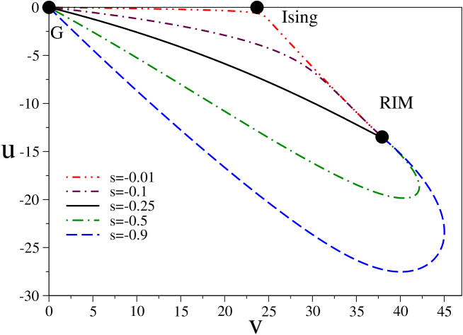
FIG. 2.: Ising systems: RG trajectories in the $(u,v)$ plane for several values of $s$ in the interval $-1<s<0$.

In Fig. 2 we show the RG trajectories for several values of $s$ in the interval $-1\lesssim s<0$, as obtained by numerically integrating the RG equations (26), after resumming the $\beta$-functions. The figure has been obtained by using a single approximant, but others give qualitatively similar results. The resummation becomes less and less effective as $|s|$ increases. This is expected since the singularities that make the perturbative series non-Borel summable play an increasingly important role as $|s|$ gets larger. In any case, for $-1\lesssim s<0$, the RG trajectories flow towards the random FP. For $s\lesssim-1$, Padé-Borel resummations (in this case we cannot use the conformal-mapping method since the singularity we use is on the positive real axis) hint at runaway RG trajectories. If this is true and not simply an artifact of the perturbative approach, this suggests the existence of a value $s_{\rm min}\approx-1$ such that systems corresponding to $s<s_{\rm min}$ do not undergo a continuous transition. As a consequence, since $u$ is directly related to the variance of disorder, the continuous transition is expected to disappear for sufficiently large disorder. This prediction may be checked by considering a lattice version of the continuum Hamiltonian

$$\int d^{3}x\;\left[{1\over 2}\left(\partial_{\mu}\varphi(x)\right)^{2}+{1\over 2}\left(t+r(x)\right)\varphi(x)^{2}+{g\over 4!}\varphi(x)^{4}\right],$$ (76)

where $\varphi$ is a scalar field and $r(x)$ is a Gaussian uncorrelated random variable. Such a model is the starting point of the FT studies of dilute systems and, by using the replica trick, can be shown to be equivalent to the model with Hamiltonian (10). Our results suggest that there is a critical value $v_{c}$ such that, if the variance of $r(x)$ is larger than $v_{c}$, the continuous transition disappears.

Beside $s=s_{\rm min}$, there is a second interesting value of $s$, the value $s^{*}$ such that the RIM FP is approached from above for $s^{*}<s<0$ and from below for $s_{\rm min}<s<s^{*}$. One can easily realize that for this particular value of $s$ the leading scaling corrections proportional to $\tau^{\Delta_{1}}$—and more generally proportional to $\tau^{n\Delta_{1}}$—are not present in the Wegner expansions of the thermodynamic quantities. Numerically, by using the conformal-mapping method, we obtain $s^{*}=-0.25(5)$.

The behavior of the RG trajectories close to the RIM FP can be determined by using the results presented in Sec. III A. We find that $v(\lambda,s)$ can be expanded as

$$v(\lambda,s)\approx v^{*}+{1\over R_{1}}(u-u^{*})-u_{\lambda,2}(s)\left({1\over R_{1}}-{1\over R_{2}}\right)\left({u-u^{*}\over u_{\lambda,1}(s)}\right)^{\omega_{2}/\omega_{1}},$$ (77)

where $R_{1}$ and $R_{2}$ are universal constants reported in Sec. III A, cf. Eq. (44), and $u_{\lambda,1}(s)$ and $u_{\lambda,2}(s)$ are expansion coefficients defined in Eq. (41). Note the presence of the nonanalytic correction which shows that, close to the FP, trajectories are only defined for $(u-u^{*})/u_{\lambda,1}(s)>0$. This is expected on the basis of general arguments [47, 48, 49]: along any RG trajectory one expects nonanalytic corrections proportional, for instance, to $n\omega_{i}/\omega_{1}+m$, $n,m$ being integers.

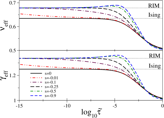
FIG. 3.: Ising systems: The effective exponents $\gamma_{\rm eff}$ and $\nu_{\rm eff}$ for several values of $s$ in the interval $-1<s<0$.

Using Eqs. (34), (35), and (36), one can compute the crossover functions $\widetilde{\xi}$ and $\widetilde{\chi}$ along the RG trajectories, i.e. for fixed $s$, and the corresponding effective exponents $\nu_{\rm eff}$ and $\gamma_{\rm eff}$, cf. Eq. (37). The effective exponents $\gamma_{\rm eff}$ and $\nu_{\rm eff}$ are shown in Fig. 3 for several values of $s<0$ within the attraction domain of the RIM FP. We note that they become nonmonotonic for $s<s^{*}\approx-0.25$, where the RG trajectories reach the RIM FP from below, see Fig. 2.

The crossover from the Gaussian FP to the RIM FP has also been investigated in Refs. [30, 14] in the framework of the minimal-subtraction scheme without $\epsilon$ expansion. The effective exponents computed here differ from those defined in Refs. [30, 14], since there the nontrivial relation between temperature and RG flow parameter was neglected. In spite of the different definitions, the crossover curves obtained in Refs. [30, 14] have the same qualitative features of those shown in Fig. 3.

The above field-theoretical results may be related with those obtained in a specific (lattice or experimental) system by comparing the behavior in a neighborhood of the critical point. Given a quantity ${\cal O}$, we can write for the field-theoretical model

$$\langle{\cal O}\rangle\approx C(s)\tau^{-\sigma}\left(1+A_{1}(s)\tau^{\Delta_{1}}+A_{2}(s)\tau^{\Delta_{2}}\right),$$ (78)

while for the lattice or experimental system we write

$$\langle{\cal O}\rangle\approx D\tau_{s}^{-\sigma}\left(1+B_{1}\tau_{s}^{\Delta_{1}}+B_{2}\tau_{s}^{\Delta_{2}}\right).$$ (79)

Then, we require these two expansions to agree apart from a rescaling of the reduced temperatures $\tau_{s}=c\tau$, i.e.

$$B_{1}=c^{\Delta_{1}}A_{1}(s),\qquad\qquad B_{2}=c^{\Delta_{2}}A_{2}(s),$$ (80)

which gives

$${A_{1}(s)\over B_{1}}=\left({A_{2}(s)\over B_{2}}\right)^{\Delta_{1}/\Delta_{2}}.$$ (81)

Thus, in order to match the two expansions one should first determine $s$ by using Eq. (81) and then fix $c$ by using Eq. (80). This provides a mapping between the field-theoretical model and the considered system. This relation does not depend on the chosen quantity ${\cal O}$ because of the universality of ratios of subleading corrections (the ratios of the $B_{1}$’s and of the $B_{2}$’s of two different quantities are universal). Note, however, that the existence of this mapping is not guaranteed. In particular, Eq. (81) requires ${A_{1}(s)/B_{1}}$ and ${A_{2}(s)/B_{2}}$ to be both positive. Since $A_{1}(s)$ changes sign for $s=s^{*}$, it is always possible to have ${A_{1}(s)/B_{1}}>0$. But there is no guarantee that ${A_{2}(s)/B_{2}}$ can always be made positive. This is the well-known sign problem that has been discussed at length in $O(M)$ models [50, 51, 52, 48]. For instance, it prevents to match the crossover curves for the scalar $\phi^{4}$ theory with the results obtained for the three-dimensional Ising model. Ref. [52] suggested the use of the “strong-coupling” branch $g>g^{*}$, but this proposal fails in the massive zero-momentum renormalization scheme because of the nonanalyticity of the RG functions at the FP [47, 48, 49]. This phenomenon is even more evident in the RIM case, cf. Eq. (77). It should also be stressed that the mapping defined by Eqs. (80) and (81) does not imply that the field-theoretical crossover curves exactly match the corresponding ones for the considered system for all values of $\tau$. In particular, there is no relation among the neglected coefficients in the Wegner expansions.

Finally, let us discuss the RIM with nearest-neighbor interactions on a cubic lattice with spin density $p$. Numerical simulations show the presence of a dilution-independent continuous transition up to $p=0.40$ [8]. It is usually conjectured that the transition persists up to the percolation threshold of the spins $p=p_{c}$, $p_{c}=0.3116081(13)$ on a cubic lattice [53]. Below the percolation point the spins form finite domains and are therefore unable to show a critical behavior. It should be remarked that the transition for $p=p_{c}$ is not described by the field-theory model (10) and thus the RIM for $p=p_{c}$ does not correspond to $s=s_{\rm min}$. For the same reasons, the fact that the transition disappears for $p<p_{c}$ does not provide evidence in favor of a finite $s_{\rm min}$. However, if the RIM can be related with the field-theory model (for example if Eq. (81) can be solved for any value of $p$) and the RIM with $p\to p_{c}$ corresponds to the field-theory model with $s\to\bar{s}$, then we can conclude $|\bar{s}|<|s_{\rm min}|$. Now we show that this condition is approximately verified. For this purpose, we must determine the relation between the RIM and the field-theory model. We use the results of Ref. [34] that map the RIM onto a translationally-invariant effective Hamiltonian ${\cal H}^{\rm RIM}_{p}$ for a field $\phi$. The expansion of ${\cal H}^{\rm RIM}_{p}$ for $\phi\to 0$ has the same form, up to order $\phi^{4}$, of the Hamiltonian (10) with $M=1$. The corresponding quartic couplings $u_{0}^{\rm RIM}$ and $v_{0}^{\rm RIM}$ appearing in this expansion are related to the magnetic concentration $p$ (note that such result does not depend on the lattice type and on the spin-spin interaction as long as it is of short-range type) by

$$u_{0}^{\rm RIM}\propto p(p-1),\qquad v_{0}^{\rm RIM}\propto p,$$ (82)

and in particular

$${u_{0}^{\rm RIM}\over v_{0}^{\rm RIM}}=-{3\over 2}(1-p).$$ (83)

It is tempting to assume $s\approx{u_{0}^{\rm RIM}/v_{0}^{\rm RIM}}$, which means that we neglect the fact that in ${\cal H}^{\rm RIM}_{p}$ there are interactions $\phi^{n}$ with any $n>4$. The relation $s\approx-3(1-p)/2$ follows. Using this relation and the numerical results of Refs. [8, 7], we can get an independent approximate estimate of $s^{*}$. Since in the RIM on a cubic lattice one does not observe the leading scaling correction for $p^{*}\approx 0.8$, we obtain $s^{*}\approx-0.3$, which is reasonably close to the FT estimate $s^{*}=-0.25(5)$. Moreover, the percolation threshold $p_{c}$—$p_{c}=0.3116081(13)$ on a cubic lattice [53]—apparently corresponds to $\bar{s}\approx-1$, which is compatible with the predicted inequality $|\bar{s}|<|s_{\rm min}|$.

B Crossover from Ising to random critical behavior

The FT approach presented in Sec. II allows us to determine also the Ising-to-RIM crossover functions. Considering in general a quantity ${\cal O}$ that behaves at the Ising FP, i.e. in the absence of disorder, as $t^{-\rho_{I}\nu_{I}}$, standard RG arguments show that, in the limit $p\to 1$ and $t\equiv(T-T_{I})/T_{I}\to 0$, where $T_{I}$ is the critical temperature of the pure Ising model, ${\cal O}$ can be written in the scaling form

$${\cal O}=a_{0}t^{-\rho_{I}\nu_{I}}B_{\cal O}\left(gt^{-\phi}\right)=a_{1}\xi^{\rho_{I}}C_{\cal O}\left(g\xi^{\phi/\nu_{I}}\right),$$ (84)

where $g\propto 1-p$ is the scaling field associated with disorder, which is a relevant perturbation of the Ising FP, and $a_{0}$ and $a_{1}$ are normalization constants. The crossover exponent $\phi$ is equal [1] to the Ising specific-heat exponent $\alpha_{I}$, $\phi=\alpha_{I}$. The functions $B_{\cal O}$ and $C_{\cal O}$ are universal, apart from trivial normalizations. By properly choosing $a_{0}$ and $a_{1}$ we can require $B_{\cal O}(0)=C_{\cal O}(0)=1$. Another condition can be added by properly fixing the normalization of $g$.

Within the FT approach the limit $g\to 0$ corresponds to $s\to 0^{-}$ and $g\xi^{\phi/\nu_{I}}\sim s\lambda^{\phi/\nu_{I}}$. Therefore, crossover functions are obtained by taking the limit $s\rightarrow 0^{-}$ and $\widetilde{\xi}=\lambda\rightarrow\infty$ of the quantity ${\cal O}\xi^{-\rho_{I}}$, keeping $s\lambda^{\alpha_{I}/\nu_{I}}$ fixed. In Fig. 4 we show numerically that such a limit exists for the susceptibility $\chi$. We consider $\chi\xi^{-2+\eta_{I}}=\widetilde{\chi}(\lambda,s)\lambda^{-2+\eta_{I}}$ and plot this combination as a function of $|s|\widetilde{\xi}^{\alpha_{I}/\nu_{I}}$ for several values of $s$. The curves, obtained by using Eq. (35) and the conformal-mapping method, rapidly converge to a limiting function.

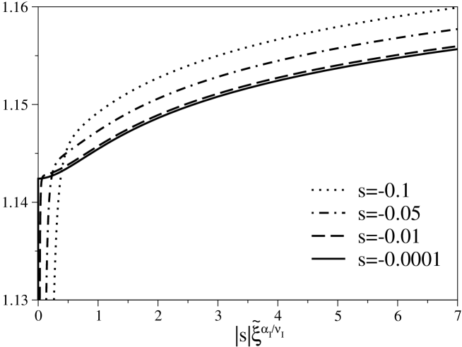
FIG. 4.: Ising systems: The quantity $\widetilde{\chi}(\lambda,s)\lambda^{-2+\eta_{I}}$ as a function of $|s|\widetilde{\xi}^{\alpha_{I}/\nu_{I}}$ for several values of $s$.

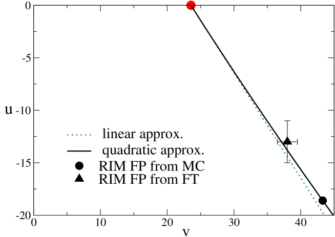
FIG. 5.: Plot of the curve $v=g(u)$. The full line represents the quadratic curve given in Eq. (88), while the dotted line shows the linear approximation $g(u)=v_{I}-u$. We also show the position of the RIM FP as obtained by MC simulations of the RIM (circle) and by FT calculations (triangle).

In order to compute the crossover functions, we must first study the limit $s\rightarrow 0^{-}$ of the RG trajectories. As it can be seen from Fig. 2, in this limit the trajectory will eventually be formed by two parts connecting at the Ising FP: the line $u=0$ starting at the Gaussian FP and ending at the Ising FP, and a line $v=g(u)$ connecting the Ising FP to the RIM FP. The line $v=g(u)$ corresponds to a RG trajectory and therefore $(u(\lambda),v(\lambda))=[u(\lambda),g(u(\lambda))]$ must satisfy Eq. (26). Therefore, $g(u)$ is the solution of the differential equation

$${dg\over du}={\beta_{v}(u,g(u))\over\beta_{u}(u,g(u))}$$ (85)

with the initial condition $g(0)=v_{I}$. As discussed in App. B, $g(u)$ is expected to be analytic for $u\to 0$ and thus it can be expanded as

$$g(u)=v_{I}+\sum_{n=1}^{\infty}g_{n}u^{n}.$$ (86)

In App. B 3 we compute the first coefficients: $g_{1}=-1$, a consequence of identity (19), $g_{2}=0.0033(1)$, and $g_{3}=1(2)\times 10^{-5}$.

Since $g(u)$ corresponds to an RG trajectory with $s=0$, Eq. (77) implies that, close to the RIM FP, we have

$$g(u)\approx v^{*}+{1\over R_{1}}(u-u^{*})-u_{\lambda,2}(0)\left({1\over R_{1}}-{1\over R_{2}}\right)\left({u-u^{*}\over u_{\lambda,1}(0)}\right)^{\omega_{2}/\omega_{1}},$$ (87)

Eq. (87) shows that $g(u)$ is not analytic at the RIM FP. Of course, one should check that $u_{\lambda,2}(0)$ does not vanish. We are not able to verify numerically this condition, but we believe that it is unlikely that $u_{\lambda,2}(0)=0$. Indeed, the curve $g(u)$ is a special curve only at the Ising FP, but it has no special status at the RIM FP and thus it should be nonanalytic as any generic RG trajectory [54].

The curve $g(u)$ can be computed [55] by resumming the perturbative series for the $\beta$ functions and then by explicitly solving Eq. (85) with the initial condition $g(0)=v_{I}$. The result turns out to be very well approximated by the simple expression

$$g(u)\approx v_{I}-u+g_{2}u^{2},$$ (88)

where $v_{I}=23.56(2)$ is the coordinate of the Ising FP [43] and $g_{2}\approx 0.0033$. Such an approximation is effective, within the resummation errors, up to the RIM FP. A graph is reported in Fig. 5. The results obtained by using [3,1], [4,1] and [5,1] Padé-Borel approximants would not be distinguishable from the curve (88) shown in Fig. 5. For instance, $g(-13)\approx 37.1$ and $g(-18.6)\approx 43.3$, so that Eq. (88) is perfectly compatible with the MC estimate of the FP, $u^{*}=-18.6(3)$, $v^{*}=43.3(2)$, and with the FT result, $u^{*}=-13(2)$, $v^{*}=38.0(1.5)$, see Fig. 5. The fact that both estimates lie on the limiting curve $v=g(u)$ shows that the FT approach is effective in determining the Ising-to-RIM trajectory, although it is apparently unable to determine precisely the position of the FP on this curve. As a final check, we compute $g^{\prime}(u^{*})$. Using Eq. (87) and the estimate of $R_{1}$ reported in Sec. III B, $R_{1}=-0.90(2)$, we obtain $g^{\prime}(u^{*})=-1.11(2)$, while Eq. (88) gives $g^{\prime}(u^{*})=-1.12$ (resp. $-1.09$) at the Monte Carlo estimate (resp. field-theoretical) of the FP. The agreement is satisfactory.

Once we have determined $g(u)$, we can compute $u(\lambda,s)$ in the crossover limit. In App. B 1, we show that, in the crossover limit, $s\rightarrow 0^{-}$ keeping $|s|\lambda^{\alpha_{I}/\nu_{I}}$ fixed, $u(\lambda,s)$ converges to $U(\sigma)$ which is implicitly defined by

$$\sigma=U(\sigma)\exp\left\{-{\alpha_{I}\over\nu_{I}}\int_{0}^{U(\sigma)}dx\;\left[{1\over\beta_{u}(x,g(x))}+{\nu_{I}\over\alpha_{I}x}\right]\right\},$$ (89)

where

$$\sigma\equiv s\Sigma_{1}\left({\lambda\over\Sigma_{2}}\right)^{\alpha_{I}/\nu_{I}},$$ (90)

and $\Sigma_{1}$ and $\Sigma_{2}$ are normalization constants such that $U(\sigma)\approx\sigma$ for $\sigma\to 0$. Their explicit expressions are reported in App. B 1. Of course, $v(\lambda,s)=g(U(\sigma))$ in the scaling limit $s\to 0^{-}$. The curve $g(u)$ and Eq. (89) completely fix the relevant RG trajectory in the crossover limit.

The computation of the crossover functions is then completely straightforward. We consider the RG function ${\cal O}(\lambda,s)$ associated with $\cal O$ and assume that it satisfies the RG equation

$$\lambda{d{\cal O}\over d\lambda}=\rho(u,v){\cal O},$$ (91)

where $\rho(u,v)$ is the corresponding RG function such that $\rho(0,v_{I})=\rho_{I}$. The crossover limit is studied in detail in App. B 2. We find that the crossover function $C_{\cal O}(y)$ can be written as

$$C_{\cal O}(y)=\exp\left[-\int_{0}^{U(\sigma)}dx\,{\rho(x,g(x))-\rho_{I}\over\beta_{u}(x,g(x))}\right],$$ (92)

where the relation between $y$ and $\sigma$ should be fixed by choosing an additional normalization condition.

We wish now to specialize the previous discussion to the magnetic susceptibility. In this case $\rho(u,v)=2-\eta_{\phi}(u,v)$. In order to completely specify the function $C_{\chi}(y)$ appearing in Eq. (84) we must fix the normalization of $g$. We use the small-$y$ expansion of $C_{\chi}(y)$. Since $C_{\chi}^{\prime}(0)=0$, see App. B 2, we require

$$C_{\chi}(y)=1+y^{2}+\sum_{n=3}c_{n}y^{n},$$ (93)

for $y\to 0$ and $C_{\chi}(y)$ to be defined for $y>0$. With these normalizations we have

$$C_{\chi}(y)=\exp\int_{0}^{U(\sigma)}dx\,{\eta_{\phi}(x,g(x))-\eta_{I}\over\beta_{u}(x,g(x))},$$ (94)

where $y=-y_{0}\sigma$. The constant $y_{0}$ is positive and is computed numerically in App. B 3: $y_{0}=0.072(8)$. The scaling function $C_{\chi}(y)$ is shown in Fig. 6.

We study the small-$y$ and large-$y$ behavior of $C_{\chi}(y)$. A rough estimate of the coefficient $c_{3}$ is $c_{3}=-4(2)$, see App. B 3. For large values of $y$, we have

$$C_{\chi}(y)\approx c_{\infty}y^{\nu_{I}(\eta_{I}-\eta)/\alpha_{I}},$$ (95)

where $\eta$ is the RIM exponent. The best estimates of the exponents $\eta_{I}$ and $\eta$ of the Ising and RIM universality classes are $\eta_{I}=0.03639(15)$ (Ref. [43]), $\eta_{I}=0.0368(2)$ (Ref. [56]), and $\eta=0.035(2)$ (Ref. [7]). These results suggest $\eta_{I}>\eta$. This is confirmed by the analysis of the fixed-dimension FT series: all analyses find $\eta_{I}>\eta$. In particular, analyses based on an expansion around the Ising FP [7] find $\eta_{I}-\eta=0.002(2)$. This suggests that $C_{\chi}(y)$ diverges for large $y$ with a very small exponent, ${\nu_{I}(\eta_{I}-\eta)/\alpha_{I}}=0.01(1)$. We also estimated the coefficient $c_{\infty}$ appearing in the large-$y$ behavior of $C_{\chi}(y)$, obtaining $c_{\infty}=1.05(5)$. We proceeded as follows. First, for given approximants of the RG functions, we computed the exponents $\eta_{I}$, $\nu_{I}$, and $\eta$, and the function $C_{\chi}(y)$. Then, we calculated $C_{\chi}(y)y^{-\nu_{I}(\eta_{I}-\eta)/\alpha_{I}}$ and determined the constant $c_{\infty}$ from its large-$y$ behavior. This procedure gave an estimate of $c_{\infty}$ for a given set of approximants. The final result was obtained as usual, by comparing the results of different approximants and of series of different order.

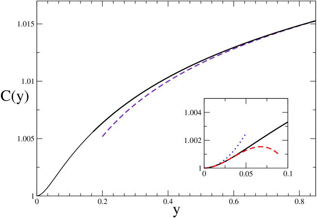
FIG. 6.: The crossover function $C_{\chi}(y)$ normalized according to Eq. (93). The dashed line represents the asymptotic behavior (95). The inset shows the small-$y$ behavior: the expansion to order $y^{2}$ corresponds to the dotted line while the expansion to order $y^{3}$ corresponds to the dashed line.

C Crossover in randomly dilute multicomponent spin systems

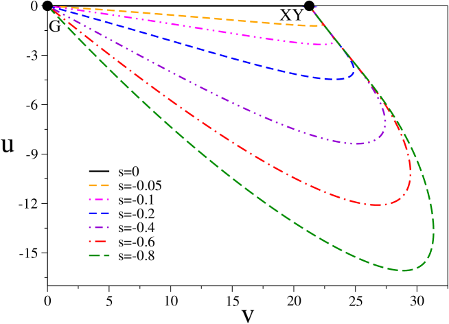
FIG. 7.: RG trajectories in the dilute XY model for $-1<s\leq 0$.

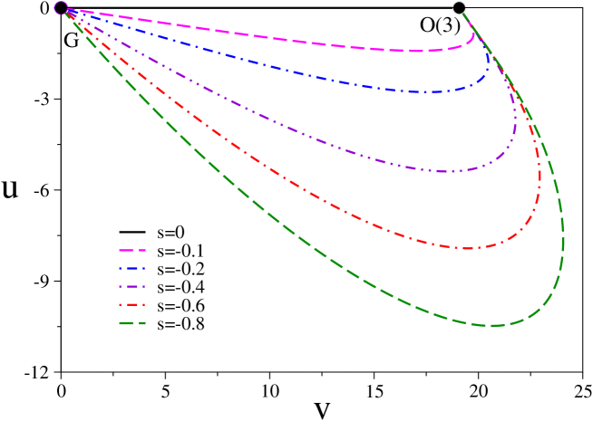
FIG. 8.: RG trajectories in the dilute Heisenberg model for $-1<s\leq 0$.

In the case of multicomponent systems, the stable FP is the O($M$)-symmetric FP $(0,v^{*})$. Precise estimates of $v^{*}$ have been obtained by employing FT and lattice techniques [4, 18, 19, 46, 57]: $v^{*}=21.16(5)$ (FT) and $v^{*}=21.14(6)$ (lattice) for the XY universality class, $v^{*}=19.06(5)$ (FT) and $v^{*}=19.13(10)$ (lattice) for the Heisenberg universality class.

In Figs. 7 and 8 we show, respectively for XY and Heisenberg systems, the RG trajectories in the $u,v$ plane for several values of $s$ in the range $-1<s\leq 0$. Figs. 9 and 10 report the corresponding effective exponents $\eta_{\rm eff}$ and $\nu_{\rm eff}$ respectively for XY and Heisenberg systems. They are nonmonotonic. In particular, for $s$ close to $-1$, $\eta_{\rm eff}$ becomes negative for intermediate values of $\tilde{\tau}$. As in the Ising case, the resummations become less reliables—and again hint at runaway trajectories—for $s\lesssim-1$.

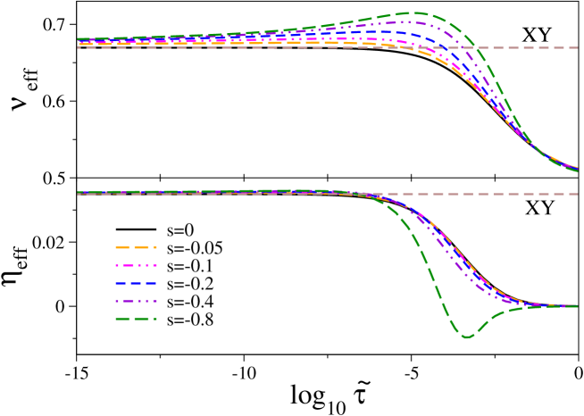
FIG. 9.: The effective exponents $\eta_{\rm eff}$ and $\nu_{\rm eff}$ of the dilute XY model for $-1<s\leq 0$. In the Gaussian limit $\nu=1/2$ and $\eta=0$, while in the Wilson-Fisher limit $\nu=0.67155(27)$ and $\eta=0.0380(4)$ (Ref. [18]).

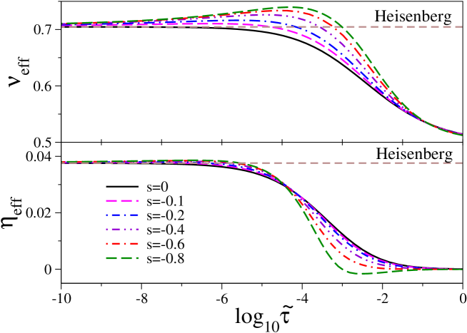
FIG. 10.: The effective exponents $\eta_{\rm eff}$ and $\nu_{\rm eff}$ of the dilute Heisenberg model for $-1<s\leq 0$. In the Gaussian limit $\nu=1/2$ and $\eta=0$, while in the Wilson-Fisher limit $\nu=0.7112(5)$ and $\eta=0.0375(5)$ (Ref. [19]).

Finally, we mention that the RG trajectories and the effective crossover exponents of dilute Heisenberg systems have been recently investigated in Ref. [31], using a two-loop approximation within the minimal-subtraction scheme without $\epsilon$ expansion and neglecting the nontrivial relation between temperature and RG flow parameter. In spite of all simplifying assumptions, the results are in qualitative agreement with ours. Moreover, Ref. [31] discusses crossover phenomena observed in experiments on isotropic magnets, showing several results for the effective exponents that are in qualitative agreement with the curves shown in Fig. 10.

A Some relations among the RG functions

In this Section we prove identities (19) and (20) holding along the $u=0$ axis, and (21), (22), and (23) holding along the $v=0$ axis.

Let us first prove the identities along the $u=0$ axis in the case $M=1$; the extension to other values of $M$ is straightforward. We consider a generic theory with fields $\phi^{A}$ and Hamiltonian density

$${\cal H}={1\over 2}\sum_{\mu,A}(\partial_{\mu}\phi^{A})^{2}+{1\over 2}r\sum_{A}(\phi^{A})^{2}+{g\over 4!}\sum_{A}(\phi^{A})^{4}+{1\over 4!}\sum_{ABCD}C_{ABCD}\phi^{A}\phi^{B}\phi^{C}\phi^{D}.$$ (A1)

For $C_{ABCD}=0$ the model is simply a collection of decoupled Ising $\phi^{4}$ theories. In order to compute the corrections to first order in $C_{ABCD}$, we consider the one-particle irreducible correlation functions of the fields expressed in terms of the bare couplings $g$ and $C_{ABCD}$ and of the inverse susceptibility $\chi^{-1}$ as effective mass (the results also hold for the massless theory in dimensional regularization)

$$\Gamma_{A_{1},\ldots,A_{n}}=\langle\phi^{A_{1}},\ldots,\phi^{A_{n}}\rangle.$$ (A2)

Then, we prove that, if all indices are equal,

$$\Gamma_{A,A,\ldots,A}=f(g)+C_{AAAA}{\partial f(g)\over\partial g}+O(C^{2})=f(g+C_{AAAA})+O(C^{2}).$$ (A3)

Using this relation, one can derive identities (19) and (20). Indeed, Eq. (A3) implies that (setting $\bar{u}_{0}\equiv u_{0}/m$ and $\bar{v}_{0}\equiv v_{0}/m$)

$$Z_{\phi}=f_{\phi}(\bar{u}_{0}+\bar{v}_{0})+O(\bar{v}_{0}^{2}),$$ (A4)

$$u+v=f_{u+v}(\bar{u}_{0}+\bar{v}_{0})+O(\bar{v}_{0}^{2}),$$ (A5)

$$\beta_{u}+\beta_{v}=f_{\beta}(\bar{u}_{0}+\bar{v}_{0})+O(\bar{v}_{0}^{2}).$$ (A6)

To prove Eq. (A3), consider a generic diagram $D$ contributing to the correlation function. If $\chi^{-1}$ is used as effective mass or the mass vanishes and dimensional regularization is used, the diagram has the following properties: it does not contain tadpole subgraphs; given a vertex $V$, the subdiagram $D/V$ obtained by deleting the lines going out of $V$ may be disconnected, but each piece contains at least one external line. The contribution of the diagram $D$ is the product of three factors: the first is the integral over the internal momenta, the second the symmetry factor, and the third one—we call it $I(D)_{A,A,\ldots,A}$—takes into account the interaction vertex

$$V_{ABCD}=-g\delta_{ABCD}-C_{ABCD}.$$ (A7)

Clearly, we are only interested in the last term which can be written in the form

$$I(D)_{A,A,\ldots,A} = \left.I(D)_{A,A,\ldots,A}\right|_{C=0}-\sum_{V\in D}\left.I(D/V)_{A,A,\ldots,A;I,J,K,L}\right|_{C=0}C_{IJKL}$$ (A8)

$$= (-g)^{n}-n(-g)^{n-1}C_{AAAA},$$ (A9)

where $n$ is the number of vertices of $D$. In the last step, we have used the two properties we have mentioned above: they guarantee that $I(D/V)_{A,A,\ldots,A;I,J,K,L}=(-g)^{n-1}\delta_{AIJKL}$, since for $C=0$ a connected diagram does not vanish only if the indices on the external legs are all equal. Eq. (A9) gives immediately Eq. (A3).

Identities (21), (22), and (23) along the $v=0$ axis can be proved in a similar fashion. Let us again restrict ourselves to the case $M=1$, the extension to generic values of $M$ being straightforward. Consider the Hamiltonian density

$${\cal H}={1\over 2}\sum_{\mu,A}(\partial_{\mu}\phi^{A})^{2}+{1\over 2}r\sum_{A}(\phi^{A})^{2}+{g\over 4!}\sum_{AB}(\phi^{A})^{2}(\phi^{B})^{2}+{1\over 4!}\sum_{ABCD}C_{ABCD}\phi^{A}\phi^{B}\phi^{C}\phi^{D},$$ (A10)

where $C_{ABCD}$ is symmetric in all indices. For $C_{ABCD}=0$ the model is simply an $N$-vector $\phi^{4}$ theory, where $N$ is the dimension of the field. In order to compute the corrections to first order in $C_{ABCD}$, we consider here a different set of correlation functions: $O(N)$-invariant (therefore there are no external indices) one-particle irreducible correlation functions of the fields and of any $O(N)$-invariant operator. Consider again a diagram $D$, a vertex $V$, and the interaction contribution $I(D/V)_{I,J,K,L}$ for $C=0$. Because of the $O(N)$ invariance, its symmetrized part is given by

$$\left.I(D/V)_{\{I,J,K,L\}}\right|_{C=0}=\hat{I}(D/V)(\delta_{IJ}\delta_{KL}+\delta_{IK}\delta_{JL}+\delta_{IL}\delta_{JK})\;.$$ (A11)

Then, repeating the argument leading to Eq. (A9), we obtain

$$I(D)=\left.I(D)\right|_{C=0}-3\sum_{V}\hat{I}(D/V)\sum_{IJ}C_{IIJJ}.$$ (A12)

The constant $\sum_{V}\hat{I}(D/V)$ is determined by computing the derivative of $I(D)$ with respect to $g$ at $C=0$.

$$\left.{\partial I(D)\over\partial g}\right|_{C=0} = \sum_{V\in D}\sum_{IJKL}\left.I(D/V)_{I,J,K,L}\right|_{C=0}\times\left(-{1\over 3}\right)(\delta_{IJ}\delta_{KL}+\delta_{IK}\delta_{JL}+\delta_{IL}\delta_{JK})$$ (A13)

$$= -\sum_{V\in D}\hat{I}(D/V)N(N+2)\;.$$ (A14)

It follows

$$I(D)=f\left(g+{3\sum_{IJ}C_{IIJJ}\over N(N+2)}\right)+O(C^{2}),$$ (A15)

where $f(g)=\left.I(D)\right|_{C=0}$. This relation is valid only for $O(N)$-invariant quantities, but it can also be applied to the correlation functions of the elementary fields by simply contracting the external indices. It allows us to derive a number of relations involving the $\beta$-functions and the RG functions associated with the exponents. For example, considering the $MN$ model (10) for $M=1$, relation (A15) implies Eqs. (21), (22), and (23) with $M=1$.

B The Ising-to-RIM crossover

In this appendix we compute the limit $s\rightarrow 0^{-}$ of the RG trajectories and the Ising-to-RIM crossover function $C_{\cal O}(y)$, cf. Eq. (84).

1 The limit $s\rightarrow 0^{-}$ of the RG trajectories

Here, we wish to prove Eqs. (89) and (90) that give $u(\lambda,s)$ in the crossover limit $s\rightarrow 0^{-}$ keeping $|s|\lambda^{\alpha_{I}/\nu_{I}}$ fixed. As discussed in Sec. IV B, in the crossover limit the RG trajectory is formed by two parts connecting at the Ising FP: the line $u=0$ starting at the Gaussian FP and ending at the Ising FP, and the line $v=g(u)$ connecting the Ising FP to the RIM FP. Now, we will solve the flow equations (26) in the two cases and we will match the two solutions in the neighborhood of the Ising FP. Let us consider first the behavior near $v=g(u)$. The flow equation for $u(\lambda,s)$ can be written as

$$-\lambda{du\over d\lambda}=\beta_{u}(u,g(u)).$$ (B1)

Since $\beta_{u}(u,v_{I})=-u\alpha_{I}/\nu_{I}$ for $u\to 0$, we can write the solution as

$$\lambda=A(s)u(\lambda,s)^{\nu_{I}/\alpha_{I}}\exp\left[-\int_{0}^{u(\lambda,s)}dx\,\left({1\over\beta_{u}(x,g(x))}+{\nu_{I}\over\alpha_{I}x}\right)\right],$$ (B2)

where $A(s)$ is a (at this stage unknown) function of $s$.

Now let us consider the second case, i.e. the trajectory near the $u=0$ axis. For $u\to 0$, we can write $\beta_{u}(u,v)=uf(v)+O(u^{2})$, with $f(0)=-1$, $f(v_{I})=-\alpha_{I}/\nu_{I}$. As for $\beta_{v}(u,v)$ we simply set $u=0$. Note that $\beta_{v}(0,v)=-v+O(v^{2})$ for $v\to 0$ and $\beta_{v}(0,v)=-\omega_{I}(v_{I}-v)$ for $v\to v_{I}$. In the limit we are interested in, the RG equations (26) become

$$-\lambda{dv\over d\lambda}=\beta_{v}(0,v),\qquad\quad-\lambda{du\over d\lambda}=uf(v).$$ (B3)

Keeping into account the initial conditions (28), we obtain

$$\lambda = v\exp\left[-\int_{0}^{v}dx\,\left({1\over\beta_{v}(0,x)}+{1\over x}\right)\right],$$ (B4)

$$u = sv\exp\int_{0}^{v}dx\,\left({f(x)\over\beta_{v}(0,x)}-{1\over x}\right).$$ (B5)

Eqs. (B4) and (B5) implicitly define $u(\lambda,s)$. We must now match the two solutions near the Ising FP, determining the unknown constant $A(s)$. If we define

$$\Sigma_{1} \equiv v_{I}\exp\int_{0}^{v_{I}}dx\,\left({f(x)\over\beta_{v}(0,x)}-{1\over x}-{\alpha_{I}\over\nu_{I}\omega_{I}(v_{I}-x)}\right),$$ (B6)

$$\Sigma_{2} \equiv v_{I}\exp\left[-\int_{0}^{v_{I}}dx\,\left({1\over\beta_{v}(0,x)}+{1\over x}+{1\over\omega_{I}(v_{I}-x)}\right)\right],$$ (B7)

for $v\to v_{I}$ Eqs. (B4) and (B5) can be written as

$$\lambda \approx \Sigma_{2}(v_{I}-v)^{-1/\omega_{I}},$$ (B8)

$$u \approx s\Sigma_{1}(v_{I}-v)^{-\alpha_{I}/\nu_{I}\omega_{I}}.$$ (B9)

Therefore, for $v\to v_{I}$ we have

$$u(\lambda,s)\approx s\Sigma_{1}\left(\lambda\over\Sigma_{2}\right)^{\alpha_{I}/\nu_{I}}.$$ (B10)

On the other hand, Eq. (B2) gives for $u\to 0$,

$$u(\lambda,s)\approx(\lambda/A(s))^{\alpha_{I}/\nu_{I}}.$$ (B11)

By comparing Eqs. (B10) and (B11) we obtain $A(s)$. Finally, Eq. (B2) can be written as

$$s\Sigma_{1}\left(\lambda\over\Sigma_{2}\right)^{\alpha_{I}/\nu_{I}}=u(\lambda,s)\exp\left[-{\alpha_{I}\over\nu_{I}}\int_{0}^{u(\lambda,s)}dx\,\left({1\over\beta_{u}(x,g(x))}+{\nu_{I}\over\alpha_{I}x}\right)\right].$$ (B12)

This ends the proof of Eqs. (89) and (90).

2 Crossover functions

The computation of the crossover function is similar to that presented in App. B 1. We first consider the RG equation (91) on the line $v=g(u)$. Using the flow equation for $u(\lambda,s)$ we can write

$${d{\cal O}\over du}=-{\rho(u,g(u))\over\beta_{u}(u,g(u))}{\cal O}.$$ (B13)

The solution can be written as

$${\cal O}=B(s)u(\lambda,s)^{\rho_{I}\nu_{I}/\alpha_{I}}\exp\left[-\int_{0}^{u(\lambda,s)}dx\,\left({\rho(x,g(x))\over\beta_{u}(x,g(x))}+{\rho_{I}\nu_{I}\over\alpha_{I}x}\right)\right],$$ (B14)

where $B(s)$ is an unknown function.

For $u\to 0$, we can use the flow equation for $v(\lambda,s)$ and write

$${d{\cal O}\over dv}=-{\rho(0,v)\over\beta_{v}(0,v)}{\cal O}.$$ (B15)

We assume $\rho(0,0)=\rho_{0}$ ($\rho_{0}$ is the naive Gaussian dimension of ${\cal O}$) and ${\cal O}\approx{\cal O}_{0}\lambda^{\rho_{0}}$ at the Gaussian FP (${\cal O}_{0}$ is a normalization constant). Then, the previous equation gives

$${\cal O}={\cal O}_{0}v^{\rho_{0}}\exp\left[-\int_{0}^{v}dx\,\left({\rho(0,x)\over\beta_{v}(0,x)}+{\rho_{0}\over x}\right)\right].$$ (B16)

Now, we must compute the behavior for $v\to v_{I}$. Defining

$$T_{1}\equiv{\cal O}_{0}v^{\rho_{0}}_{I}\exp\left[-\int_{0}^{v_{I}}dx\,\left({\rho(0,x)\over\beta_{v}(0,x)}+{\rho_{0}\over x}+{\rho_{I}\over\omega_{I}(v_{I}-x)}\right)\right],$$ (B17)

we obtain for $v\to v_{I}$

$${\cal O}\approx T_{1}(v_{I}-v)^{-\rho_{I}/\omega_{I}}\approx T_{1}\left(\lambda\over\Sigma_{2}\right)^{\rho_{I}}\approx T_{1}\left({u\over s\Sigma_{1}}\right)^{\nu_{I}\rho_{I}/\alpha_{I}},$$ (B18)

where we have used Eq. (B9). On the other hand, Eq. (B14) gives in the limit $u\to 0$

$${\cal O}\approx B(s)u^{\nu_{I}\rho_{I}/\alpha_{I}}.$$ (B19)

Therefore,

$${\cal O}=T_{1}\left({u\over s\Sigma_{1}}\right)^{\nu_{I}\rho_{I}/\alpha_{I}}\exp\left[-\int_{0}^{u(\lambda,s)}dx\,\left({\rho(x,g(x))\over\beta_{u}(x,g(x))}+{\rho_{I}\nu_{I}\over\alpha_{I}x}\right)\right].$$ (B20)

Finally, by using Eq. (B12) to eliminate $u^{\nu_{I}\rho_{I}/\alpha_{I}}$, we obtain

$${\cal O}=T_{1}\Sigma_{2}^{-\rho_{I}}\lambda^{\rho_{I}}\exp\left[-\int_{0}^{U(\sigma)}dx\;{\rho(x,g(x))-\rho_{I}\over\beta_{u}(x,g(x))}\right].$$ (B21)

The crossover function $C_{\cal O}(y)$ normalized so that $C_{\cal O}(0)=1$ is then given by

$$C_{\cal O}(y)=\exp\left[-\int_{0}^{U(\sigma)}dx\;{\rho(x,g(x))-\rho_{I}\over\beta_{u}(x,g(x))}\right].$$ (B22)

To fully specify the function $C_{\cal O}(y)$ we must also relate $y$ with $\sigma$ by adding an additional normalization condition. For the magnetic susceptibility this is done in detail in Sec. IV B.

We can specialize these results to the observables we have considered in the paper. First, we consider the four-point quartic couplings $G_{22}$ and $G_{4}$. Since they are related to $u$ and $v$, $G_{22}={u/3}$ and $G_{4}=v$ (see Ref. [41]), and $u\approx U(\sigma)$, $v\approx g(u)$ in the crossover limit, we obtain

$$C_{G_{22}}(y)={U(\sigma)\over\sigma},$$ (B23)

$$C_{G_{4}}(y)={1\over v_{I}}g(U(\sigma)).$$ (B24)

Note that $C_{G_{22}}(y)$ is not simply $U(\sigma)$ since the crossover function is defined by $u\sim\lambda^{\alpha_{I}/\nu_{I}}C_{G_{22}}(y)$. These equations can also be derived from Eq. (B22) bu using $\rho(u,v)=-\beta_{u}(u,v)/u$ and $\rho(u,v)=-\beta_{v}(u,v)/v$ for $u$ and $v$ respectively.

Finally, let us consider the magnetic susceptibility $\chi$. In this case $\rho(u,v)=2-\eta_{\phi}(u,v)$. Thus, by using Eq. (B22) we obtain Eq. (94). Let us now show that ${C}_{\chi}^{\prime}(0)=0$. First, note that, because of identity (20), near the Ising FP we have

$$\eta_{\phi}(u,v)-\eta_{I}=A(u+v-v_{I})[1+O(u)+O(v-v_{I})],$$ (B25)

where $A$ is a constant. Then, since $g(u)=v_{I}-u+O(u^{2})$, we obtain $\eta_{\phi}(u,g(u))-\eta_{I}=O(u^{2})$. Substituting in Eq. (94), this gives immediately $C_{\chi}^{\prime}(0)=0$.

Finally, we argue that the crossover function $C_{\cal O}(y)$ and $g(u)$ (that can be related to the crossover function of $v=G_{4}$) are analytic for $y\to 0$ and $u\to 0$ respectively. This is not obvious since for $u=0$ RG functions are nonanalytic at the Ising FP [47, 49]. We will now show that such a problem does not arise for the RG functions defined along the crossover line $v=g(u)$. The reason is that such a line has a very special status at the Ising FP: It is the line that is tangent to the relevant direction associated with disorder and that is orthogonal to all irrelevant directions.

To clarify the issue, let us for instance consider the singular part of the free energy. In a neighborhood of the Ising FP it can be written as [58]

$$F_{\rm sing}=f_{t}^{d/\nu_{I}}F\left(f_{p}f_{t}^{-\phi},\{f_{i}f_{t}^{\Delta_{i}}\}\right),$$ (B26)

where $f_{t}$, $f_{p}$, and $\{f_{i}\}$ are the nonlinear scaling fields associated with the temperature, the dilution, and the irrelevant RG operators. For $t\equiv(T-T_{I})/T_{I}\to 0$ and $p\to 1$, $f_{t}\sim t$ and $f_{p}\sim(1-p)\sim g$. The exponents $\Delta_{i}$ are associated with the irrelevant operators and are positive. A basic result of RG theory is that the nonlinear scaling fields are analytic in $t$ and $p$ and the function $F$ is analytic in all its arguments. In the crossover limit, $f_{i}$ approaches a constant and $f_{t}$ goes to zero, so that $f_{i}f_{t}^{\Delta_{i}}\to 0$. It follows

$$F_{\rm sing}\approx t^{d/\nu_{I}}F(gt^{-\phi},\{0\}),$$ (B27)

which shows that the crossover function associated with $F_{\rm sing}$ is analytic in $gt^{-\phi}$. The argument can be trivially generalized to any zero-momentum quantity; we conjecture that it also applies to quantities involving the correlation length.

3 Some numerical results

In this Section we report some details on the numerical computation of $g(u)$ and $C_{\chi}(y)$. Let us first focus on the determination of the coefficients $g_{n}$ defined in Eq. (86). They have been obtained by resumming perturbative series $g_{n}(v)$ such that $g_{n}=g_{n}(v_{I})$. For the purpose of determining $g_{n}(v)$, we write

$$\beta_{u}(u,v) = \sum_{n}b_{u,n}(v)u^{n},$$ (B28)

$$\beta_{v}(u,v) = \sum_{n}b_{v,n}(v)u^{n}.$$ (B29)

Then, by using Eq. (85), we obtain

$$g_{2}=\left.{b_{v,0}^{\prime\prime}(v)-2b_{v,2}(v)-2b_{u,2}(v)\over 2[\alpha_{I}/\nu_{I}+b_{v,1}(v)]}\right|_{v=v_{I}},$$ (B30)

and similar, but more complex, expressions for $g_{3}$, $g_{4}$, etc. The series $g_{n}(v)$ can be obtained by expanding the right-hand side in powers of $v$. For $g_{2}$ and $g_{3}$ we obtain

$$g_{2}(\bar{v}) = 0.00663146-0.00693165\bar{v}+0.0116887\bar{v}^{2}-0.0225971\bar{v}^{3}+$$ (B32)

$$+0.0455962\bar{v}^{4}-0.0954011\bar{v}^{5}+O(\bar{v}^{6}),$$

$$g_{3}(\bar{v}) = 0.0000293176-0.0000813454\bar{v}+0.000206937\bar{v}^{2}-0.000485549\bar{v}^{3}+$$ (B34)

$$+0.00110105\bar{v}^{4}+O(\bar{v}^{5}),$$

where $\bar{v}\equiv 3v/(16\pi)$. By resumming these series we get

$$g_{2}=0.0033(1),\qquad g_{3}=1(2)\times 10^{-5}.$$ (B35)

We computed the function $g(u)$ by using Eq. (85), i.e. without relying on an expansion around the Ising FP, and by resumming the $\beta$-functions using [3/1], [4/1], and [5/1] Padè-Borel approximants constrained to have a zero at $v=v_{I}=23.56$. The results up to $u\approx-20$ would not be distinguishable from the quadratic approximation shown in Fig. 5.

Let us now consider $C_{\chi}(y)$. This function can be computed directly by using Eqs. (89) and (94). They provide $C_{\chi}$ as a function of the variable $\sigma$. In order to compute the relation between $\sigma$ and $y$, we need to determine the small-$\sigma$ behavior of $C_{\chi}$. We write

$$C_{\chi}=1+\sum_{n=2}\overline{c}_{n}\sigma^{n},$$ (B36)

and, as for $g(u)$, we compute perturbative series $\overline{c}_{n}(v)$ such that $\overline{c}_{n}=\overline{c}_{n}(v_{I})$. By resumming these expansions we obtain

$$\overline{c}_{2}=0.0052(12),\qquad c_{3}=\overline{c}_{3}\overline{c}_{2}^{-3/2}=-4(2).$$ (B37)

The variable $y$ defined by the normalization condition (93) is related to $\sigma$ by $y=-\overline{c}_{2}^{1/2}\sigma=-0.072(8)\,\sigma$.

REFERENCES

- [1] A. Aharony, in Phase Transitions and Critical Phenomena, edited by C. Domb and M. S. Green (Academic Press, New York, 1976), Vol. 6, p. 357.
- [2] R. B. Stinchcombe, in Phase Transitions and Critical Phenomena, edited by C. Domb and J. Lebowitz (Academic Press, New York, 1983), Vol. 7, p. 152.
- [3] D. P. Belanger, Brazilian J. Phys. 30, 682 (2000) [cond-mat/0009029].
- [4] A. Pelissetto and E. Vicari, Phys. Rep. 368, 549 (2002).
- [5] R. Folk, Yu. Holovatch, and T. Yavors’kii, Usp. Fiz. Nauk 173, 175 (2003) [Phys. Usp. 46, 175 (2003)].
- [6] In pure uniaxial antiferromagnets a uniform magnetic field does not change the nature of the critical transition for , where the critical value corresponds to a multicritical point [J. M. Kosterlitz, D. R. Nelson, and M. E. Fisher, Phys. Rev. Lett. 33, 813 (1974), Phys. Rev. B 13, 412 (1976)]. On the other hand, in the presence of dilution, for any the transition does not belong the the RIM universality class but rather to the same universality class of the transition of the random-field Ising model. See: S. Fishman and A. Aharony, J. Phys. C 12, L729 (1979) and D. P. Belanger, in Spin Glasses and Random Fields, edited by A. P. Young (World Scientific, Singapore, 1998), p. 251. The crossover exponent that controls the behavior in the limit has been recently estimated by computing and analyzing six-loop series in the framework of the fixed-dimension FT expansion [P. Calabrese, A. Pelissetto, and E. Vicari, Phys. Rev. B 68, 092409 (2003)].
- [7] P. Calabrese, V. Martín-Mayor, A. Pelissetto, and E. Vicari, Phys. Rev. E 68, 036136 (2003).
- [8] H. G. Ballesteros, L. A. Fernández, V. Martín-Mayor, A. Muñoz Sudupe, G. Parisi, and J. J. Ruiz-Lorenzo, Phys. Rev. B 58, 2740 (1998).
- [9] S. Wiseman and E. Domany, Phys. Rev. Lett. 81, 22 (1998); Phys. Rev. E 58, 2938 (1998).
- [10] W. Selke, L. N. Shchur, and A. L. Talapov, in Annual Reviews of Computational Physics, Vol. I, edited by D. Stauffer (World Scientific, Singapore, 1995).
- [11] A. Pelissetto and E. Vicari, Phys. Rev. B 62, 6393 (2000).
- [12] P. Calabrese, A. Pelissetto, P. Rossi, E. Vicari, hep-th/0212161, Talk at the International Conference on Theoretical Physics, TH-2002, UNESCO, Paris, 2002.
- [13] D. V. Pakhnin and A. I. Sokolov, Phys. Rev. B 61, 15130 (2000).
- [14] R. Folk, Yu. Holovatch, and T. Yavors’kii, Phys. Rev. B 61, 15114 (2000).
- [15] B. N. Shalaev, S. A. Antonenko, and A. I. Sokolov, Phys. Lett. A 230, 105 (1997).
- [16] M. Tissier, D. Mouhanna, J. Vidal, and B. Delamotte, Phys. Rev. B 65, 140402 (2002).
- [17] A. B. Harris, J. Phys. C 7, 1671 (1974).
- [18] M. Campostrini, M. Hasenbusch, A. Pelissetto, P. Rossi, and E. Vicari, Phys. Rev. B 63, 214503 (2001).
- [19] M. Campostrini, M. Hasenbusch, A. Pelissetto, P. Rossi, and E. Vicari, Phys. Rev. B 65, 144520 (2002).
- [20] J. Yoon and M. H. W. Chan, Phys. Rev. Lett. 78, 4801 (1997).
- [21] G. M. Zassenhaus and J. D. Reppy, Phys. Rev. Lett. 83, 4800 (1999).
- [22] S. N. Kaul, J. Magn. Magn. Mater. 53, 5 (1985).
- [23] S. N. Kaul and M. Sambasiva Rao, J. Phys.: Condens. Matter 6, 7403 (1994).
- [24] P. D. Babu and S. N. Kaul, J. Phys.: Condens. Matter 9, 7189 (1997).
- [25] V. L. Ginzburg, Fiz. Tverd. Tela 2, 2031 (1960) [Sov. Phys. Solid State 2, 1824 (1960)].
- [26] E. Luijten and K. Binder, Phys. Rev. E 58, R4060 (1998); 59, 7254 (1999); A. Pelissetto, P. Rossi, and E. Vicari, Phys. Rev. E 58, 7146 (1998); Nucl. Phys. B 554, 552 (1999); S. Caracciolo, M. S. Causo, A. Pelissetto, P. Rossi, and E. Vicari, Phys. Rev. E 64, 046130 (2001).
- [27] C. Bagnuls and C. Bervillier, Phys. Rev. B 32, 7209 (1985); Phys. Rev. E 65, 066132 (2002).
- [28] R. Schloms and V. Dohm, Nucl. Phys. B 328, 639 (1989).
- [29] H. J. Krause, R. Schloms, and V. Dohm, Z. Phys. B 79, 287 (1990).
- [30] H. K. Janssen, K. Oerding, and E. Sengespeick, J. Phys. A 28, 6073 (1995).
- [31] M. Dudka, R. Folk, Yu. Holovatch, and D. Ivaneiko, J. Magn. Magn. Mater. 256, 243 (2003).
- [32] V. J. Emery, Phys. Rev. B 11, 239 (1975).
- [33] S. W. Edwards and P. W. Anderson, J. Phys. F 5, 965 (1975).
- [34] G. Grinstein and A. Luther, Phys. Rev. B 13, 1329 (1976).
- [35] A. Aharony, Y. Imry, and S. K. Ma, Phys. Rev. B 13 466 (1976).
- [36] D. Mukamel and G. Grinstein, Phys. Rev. B 25, 381 (1982).
- [37] J. M. Carmona, A. Pelissetto, and E. Vicari, Phys. Rev. B 61, 15136 (2000).
- [38] P. Calabrese, A. Pelissetto, and E. Vicari, Phys. Rev. B 67, 024418 (2003).
- [39] A. J. Bray, T. McCarthy, M. A. Moore, J. D. Reger, and A. P. Young, Phys. Rev. B 36, 2212 (1987); A. J. McKane, Phys. Rev. B 49, 12003 (1994).
- [40] G. Álvarez, V. Martín-Mayor, and J. J. Ruiz-Lorenzo, J. Phys. A 33, 841 (2000).
- [41] P. Calabrese, M. De Prato, A. Pelissetto, and E. Vicari, Phys. Rev. B 68, 134418 (2003).
- [42] In detail we obtain: (conformal mapping; field-theoretical estimate of the FP); (Padé-Borel; field-theoretical estimate of the FP); (conformal mapping; Monte Carlo estimate of the FP). No estimate at the Monte Carlo FP could be obtained by using the Padé-Borel method: indeed, different approximants show large fluctuations. At the field-theoretical estimate of the FP has been computed in two different ways: one can resum its perturbative expansion; one can first resum the -functions and then differentiate the resummed expressions, computing the stability matrix and its eigenvalues. At the Monte Carlo estimate of the FP only the first method has been used. Both methods have also been used in the analysis of and at the field-theoretical estimate of the FP.
- [43] M. Campostrini, A. Pelissetto, P. Rossi, and E. Vicari, Phys. Rev. E 65, 066127 (2002); Phys. Rev. E 60, 3526 (1999).
- [44] P. Butera and M. Comi, Phys. Rev. B 65, 144431 (2002).
- [45] J. Kyriakidis and D.J.W. Geldart, Phys. Rev. B 53, 11572 (1996).
- [46] A. Pelissetto and E. Vicari, Nucl. Phys. B 575, 579 (2000);
- [47] B. G. Nickel, in Phase Transitions, edited by M. Lévy, J. C. Le Guillou, and J. Zinn-Justin (Plenum, New York-London, 1982).
- [48] A. D. Sokal, Europhys. Lett. 27, 661 (1994); erratum 30, 123 (1995).
- [49] A. Pelissetto and E. Vicari, Nucl. Phys. B 519, 626 (1998).
- [50] A. J. Liu and M. E. Fisher, J. Stat. Phys. 58, 431 (1990).
- [51] B. J. Nickel, Macromolecules 24, 1358 (1991).
- [52] L. Schäfer, Phys. Rev. E 50, 3517 (1994).
- [53] H. G. Ballesteros, L. A. Fernández, V. Martín-Mayor, A. Muñoz Sudupe, G. Parisi, and J. J. Ruiz-Lorenzo, J. Phys. A 32, 1 (1999).
- [54] This is essentially the argument of Sokal (Ref. [48]) for the nonanalyticity of the -function at a FP. A numerical example illustrating these ideas is given in App. E of B. Li, N. Madras, and A. D. Sokal, J. Stat. Phys. 80, 661 (1995).
- [55] The Ising-to-RIM trajectory can be also characterized by the equation , where has been defined in Eq. (15), or equivalently by the fact that along it and diverge [P. Parruccini and P. Rossi, Phys. Rev. E 64, 047104 (2001)].
- [56] Y. Deng and H. W. J. Blöte, Phys. Rev. E 68, 036125 (2003).
- [57] R. Guida and J. Zinn-Justin, J. Phys. A 31, 8103 (1998).
- [58] F. J. Wegner, in Phase Transitions and Critical Phenomena, edited by C. Domb and M. S. Green (Academic Press, New York, 1976), Vol. 6.