On observability of Rényi’s entropy

Abstract

Despite recent claims we argue that Rényi’s entropy is an observable quantity. It is shown that, contrary to popular belief, the reported domain of instability for Rényi entropies has zero measure (Bhattacharyya measure). In addition, we show the instabilities can be easily emended by introducing a coarse graining into an actual measurement. We also clear up any doubts regarding the observability of Rényi’s entropy in (multi–)fractal systems and in systems with absolutely continuous probability density functions.

PACS: 65.40.Gr, 47.53.+n, 05.90.+m
Keywords: Rényi’s information entropy; Lesche’s observability condition; Bhattacharyya measure

Abstract

I Introduction

Thermodynamical or statistical concept of entropy, though deeply rooted in physics, is rigorously defined only for equilibrium systems or, at best, for adiabatically evolving systems. In fact, the very existence of the entropy in thermodynamics is attributed to Carathéodory’s inaccessibility theorem [1] and the statistical interpretation behind the thermodynamical entropy is then usually provided via the ergodic hypothesis [2, 3]. It is, however, highly non–trivial matter to find a proper conceptual ground for entropy of systems away from equilibrium, non–ergodic systems or equilibrium systems with “exotic” non–Gibbsian statistics (multifractals, percolation, polymers or protein folding provide examples). It is frequently said that entropy is a measure of disorder, and while this needs many qualifications and clarifications it is generally believed that this does represent something essential about it. Information theory might be then viewed as a pertinent mathematical framework capable of quantifying the “measure of disorder”. It is undoubted advantage of information theoretic approaches that whenever one can measure (or control) information one can also measure (or control) the associated entropy, as the latter is essentially an average information about a system in question [4, 5].

In recent years there have been many attempts to extend the equilibrium concept of entropy to more generic situations applying various generalizations of the information theory. Systems with (multi–)fractal structure, long–range interactions and long–time memories might serve as examples. Among multitude of information entropies Shannon’s entropy, Rényi entropies and Tsallis–Havrda–Charvat (THC) non–extensive entropies [6] have found utility in a wide range of physical problems. Shannon’s entropy is known to reproduce the usual Gibbsian thermodynamics and is frequently used in such areas as astronomy, geophysics, biology, medical diagnosis and economics (for the latest developments in Shannon’s entropy applications the interested reader may consult Ref. [7] and citations therein). Rényi entropies were conveniently applied, for instance, in multiparticle hadronic systems [8], fractional diffusion processes [9] or in multifractal systems [10]. THC entropy was recently used in a study of systems with strong long–range correlations and in systems with long–time memories[11].

Despite the information theoretic origin there has been raised some doubt regarding the observability of Rényi entropies [12]. Some authors went even as far as to claim that instabilities in systems with large number of microstates completely invalidate use of Rényi entropies in all physical problems [13]. This is rather surprising since Rényi’s entropy is routinely measured in numerous situation ranging from coding theory and cryptography [14] (where it regulates the optimality of coding), through chaotic dynamical systems [10] (where it determines the generalized dimensions for strange attractors) and earthquake analysis [15] (where it is used to evaluate the distribution of earthquake epicenters and lacunarity) to non–parametric mathematical statistics (where it prescribes the price of constituent information). Besides, Rényi entropies directly provide measurable bounds in quantum–information uncertainty relations [16].

In the present paper we aim to revise Lesche’s condition of observability. We illustrate this in various contexts; systems with finite number of microstates, systems with infinite (but countable) number of microstates, systems with absolutely continuous probability density functions (PDF’s) and multifractals. We show that it is not quite as simple to define the ubiquitous concept of observability. We propose a less restrictive observability condition and demonstrate that Rényi entropies are observable in this new framework. In what follows we will give some considerations in favor of the above statement.

The paper is organized in the following way: In Section II we discuss Lesche’s criterion of observability which frequently forms a core argument against observability of Rényi entropies. We argue that the criterion is unnecessary restrictive and, in fact, many standard physical phenomena which are observed and measured in a real world do not obey Lesche’s condition. In Section III we present some essentials of Rényi entropies required in the main body of the paper. In Section IV A we argue that for the finite number of microstates Rényi entropies easily conform with Lesche’s criterion, i.e., they are observable. In Section IV B we extend our analysis to a countably infinite number of microstates. Here appearance of instabilities may be observed. The latter can be traced to a large sensitivity of Rényi entropies to (ultra)rare–event systems. We demonstrate that when the coarse graining is included into realistic measurements, the instabilities get “diluted” and Rényi entropies once again obey Lesche’s condition. In Section IV C we propose more realistic criterion of observability where we allow for a certain amount of instability points, provided the latter ones have measure zero. To this extend we employ Bhattacharyya statistical measure - i.e., natural measure on the space of non–parametric statistics. We prove that the Bhattacharyya measure of the above “critical” distributions is in fact zero. Finally, we analyze in Section V systems with continuous probability distributions and multifractal systems. We find that the very nature of the absolute continuity of PDF’s and the multifractality prohibits per se an appearance of instability points.

II Lesche’s criterion of observability

In order to explain fully the apparent inconsistencies in the recent claims concerning non–observability of Rényi entropies we feel it is necessary to briefly review the main points of Lesche’s observability criterion. While we hope to discuss all the salient points, a full discussion can be obtained in Lesche [12]. Our discussion will be in terms of a scalar quantity $G({\boldsymbol{x}})$. Following [12], a necessary condition for $G({\boldsymbol{x}})$ with the state variable ${\boldsymbol{x}}\in X\subset{\mathbb{R}}^{n}$ to be observable is following: Let

$$||{\boldsymbol{x}}-{\boldsymbol{x}}^{\prime}||_{1}=\sum_{k}^{n}|x_{k}-x^{\prime}_{k}|\,,$$

be the Hölder $l_{1}$–metric on ${\mathbb{R}}^{n}$, then for $\forall\varepsilon>0$ there exists (${\boldsymbol{x}}$–independent) $\delta_{\varepsilon}>0$ such that for any pair ${\boldsymbol{x}}$, ${\boldsymbol{x}}^{\prime}$ one has

$$||{\boldsymbol{x}}-{\boldsymbol{x}}^{\prime}||_{1}\leq\delta_{\varepsilon}\ \Rightarrow\ \frac{|G({\boldsymbol{x}})-G({\boldsymbol{x}}^{\prime})|}{G_{max}}<\varepsilon\,.$$ (1)

From a strict mathematical standpoint (1) is, in fact, the definition of the uniform metric continuity of $G({\boldsymbol{x}})$ on the state space $X$. Informally Eq.(1) states that points from $X$ which are close in sense of $||\ldots||_{1}$ are mapped via $G$ to points which are close in $|\ldots|$ metric. Lesche’s criterion is thus nothing but the condition of stability of $G({\boldsymbol{x}})$ under a measurement. In fact, the continuity criterion ensures that a small error in a state variable ${\boldsymbol{x}}$ will not bring in repeated experiments violent fluctuations in measured data. The uniform continuity in Eq.(1) is then a key ingredient to secure that the size of the changes in $G({\boldsymbol{x}})$ depends only on the size of the changes in ${\boldsymbol{x}}$ but not on ${\boldsymbol{x}}$ itself. This condition excludes, for example, systems whose statistical fluctuations in $G({\boldsymbol{x}})$ would change too dramatically with a small change in the state variable ${\boldsymbol{x}}$.

When $G({\boldsymbol{x}})$ is bounded we can recast Lesche’s condition of observability into equivalent but more expedient form, namely (inverse) Lipschitz continuity condition [17]. In this case, a quantity $G:X\subset{\mathbb{R}}^{n}\mapsto\mathbb{R}$ is observable in Lesche’s sense if and only if for every $\varepsilon>0$ there exists (${\boldsymbol{x}}$–independent and finite) $K_{\varepsilon}$ such that for any pair ${\boldsymbol{x}}$, ${\boldsymbol{x}}^{\prime}\in X$ one has

$$|G({\boldsymbol{x}})-G({\boldsymbol{x}}^{\prime})|\leq K_{\varepsilon}||{\boldsymbol{x}}-{\boldsymbol{x}}^{\prime}||_{1}+\varepsilon\,.$$ (2)

We will practically employ the condition (2) in Section IV A.

Criteria (1) and (2) get generalized in case when $n\rightarrow\infty$. This should be expected as the uniform continuity may not survive in the large $n$ limit. To avoid such situations Lesche postulated that the mapping

$$G:\bigcup_{n=1}^{\infty}X_{n}\mapsto{\mathbb{R}}\,,$$ (3)

with $X_{n}\subset{\mathbb{R}}^{n}$, taken as a function of $n$, converges to an uniformly continuous function in an uniform manner, i.e., for $\forall\varepsilon>0$ there exists $\delta_{\varepsilon}>0$ such that for $\forall$ ${\boldsymbol{x}},{\boldsymbol{x}}^{\prime}\in{\mathbb{R}}^{n}$ and $\forall n\in{\mathbb{Z}}^{+}$

$$||{\boldsymbol{x}}-{\boldsymbol{x}}^{\prime}||_{1}\leq\delta_{\varepsilon}\ \Rightarrow\ \frac{|G({\boldsymbol{x}})-G({\boldsymbol{x}}^{\prime})|}{G_{max}}<\varepsilon\,.$$ (4)

The uniform convergence is then reflected in the fact that $\delta_{\varepsilon}$ is both ${\boldsymbol{x}}$ and $n$ independent.

Let us add a couple of remarks concerning the aforementioned observability conditions. Lesche’s condition, as illustrated above, is based on the notion of measurability. This is however not the only possible way how to define observability. It is well known that various alternative concepts exist in literature. For instance, one may use the approach based on distinguishability [18] or detectability [19]. In fact, the condition based on measurability, and namely the condition of uniform continuity, might be often to tight. Indeed, there are clearly many quantities which are not uniformly continuous in their state variables (e.g., they are discontinuous in finite number of points in the state space) and which are, nevertheless, perfectly detectable and well defined away from the singularity domain. Note, for instance, that although pressure and latent heat in 1st order phase transitions are discontinuous in temperature, and similarly susceptibility in 2nd order phase transitions is nonanalytic in temperature, there is still no reason to dismiss pressure, latent heat and susceptibility as observables. Discontinuous or nonanalytic state functions are not exclusive to phase transitions only. Actually, such a type of behavior is common to many different situations - formation of shocks in nonlinear wave propagation, mechanical systems involving small masses and large damping, electric–circuit systems with large resistance and small inductance, catastrophe and bifurcation theories, to name a few.

III Rényi entropies

Rényi entropies constitute a one–parametric family of information entropies labelled by Rényi’s parameter $\alpha\in{\mathbb{R}}^{+}$ and fulfill the additivity with respect to the composition of statistically independent systems. The special case with $\alpha=1$ corresponds to ordinary Shannon’s entropy. It might be shown that Rényi entropies belong to the class of mixing homomorphic functions [12] and that they are analytic for $\alpha$’s which lie in $I\cup IV$ quadrants of the complex plane [20]. In order to address the observability issue it is important to distinguish three situations.

A Discrete probability distribution case

Let ${\mathcal{X}}=\{x_{1},\ldots,x_{n}\}$ be a random variable admitting $n$ different events (be it outcomes of some experiment or microstates of a given macrosystem), and let ${\mathcal{P}}=\{p_{1},\ldots,p_{n}\}$ be the corresponding probability distribution. Information theory then ensures that the most general information measures (i.e., entropy) compatible with the additivity of independent events are those of Rényi [4]:

$${\cal{I}}_{\alpha}({\cal{P}})=\frac{1}{(1-\alpha)}\,\mbox{log}_{2}\left(\sum_{k=1}^{n}p^{\alpha}_{k}\right)\,.$$ (5)

Form (5) is valid even in the limiting case when $n\rightarrow\infty$. If, however, $n$ is finite then Rényi entropies are bounded both from below and from above: $\log_{2}(p_{k})_{\mbox{{max}}}\leq{\cal{I}}_{\alpha}\leq\log_{2}n.$ In addition, Rényi entropies are monotonically decreasing functions in $\alpha$, so namely ${\cal{I}}_{\alpha_{1}}<{\cal{I}}_{\alpha_{2}}$ if and only if $\alpha_{1}>\alpha_{2}$. One can reconstruct the entire underlying probability distribution knowing all Rényi distributions via Widder–Stiltjes inverse formula [20]. In the latter case the leading order contribution comes from ${\cal{I}}_{1}({\cal{P}})$, i.e., from Shannon’s entropy. Typical playground of (5) is in a coding theory [21], cryptography [14] and in theory of statistical inference [4]. The parameter $\alpha$ might be then related with the price of constituent information. It should be admitted that in discrete cases the conceptual connection of ${\cal{I}}_{\alpha}({\cal{P}})$ with actual physical problems is still an open issue. The interested reader can find some further practical applications of discrete Rényi entropies, for instance, in [20, 22]

B Continuous probability distribution case

Let $M$ be a support on which is defined a continuous PDF ${\mathcal{F}}({\boldsymbol{x}})$. We will assume that the support (or outcome space) can be generally a fractal set. By covering the support with the mesh $M^{(l)}$ of $d$–dimensional (disjoint) cubes $M^{(l)}_{k}$ $(k=1,\ldots,n)$ of size $l^{d}$ we may define the integrated probability in $k$–th cube as

$$p_{nk}={\mathcal{F}}({\boldsymbol{x}}_{i})l^{d}\,,\;\;\;{\boldsymbol{x}}_{i}\in M_{k}^{(l)}\,.$$ (6)

The latter specifies the mesh probability distribution ${\mathcal{P}}_{n}=\{p_{n1},\ldots,p_{nn}\}$. Infinite precision of measurements (i.e., with $l\rightarrow 0$) often brings infinite information. In fact, it is more sensible to consider the relative information entropy rather than absolute one as the most “junk” information comes from the uniform distribution ${\mathcal{E}}_{n}$. It was shown in [4, 20] that in the $n\rightarrow\infty$ (i.e., $l\rightarrow 0$) limit it is possible to define finite information measure compatible with information theory axioms. This renormalized Rényi’s entropy - negentropy (or information gain), reads

$$\tilde{{\cal{I}}}_{\alpha}({\cal{F}}) \equiv \lim_{n\rightarrow\infty}({\cal{I}}_{\alpha}({\cal{P}}_{n})-{\cal{I}}_{\alpha}({\cal{E}}_{n}))\ =\ \frac{1}{(1-\alpha)}\,\log_{2}\left(\frac{\int_{M}d\mu\,{\cal{F}}^{\alpha}({\boldsymbol{x}})}{\int_{M}d\mu\,1/V^{\alpha}}\right)\,.$$ (7)

Here $V$ is the corresponding volume. Eq.(7) can be viewed as a generalization of the Kullback–Leibler relative entropy [24]. It is possible to introduce a simpler alternative prescription as

$${\cal{I}}_{\alpha}({\cal{F}}) \equiv \lim_{n\rightarrow\infty}({\cal{I}}_{\alpha}({\cal{P}}_{n})-{\cal{I}}_{\alpha}({\cal{E}}_{n})|_{V=1})\ =\ \lim_{n\rightarrow\infty}({\cal{I}}_{\alpha}({\cal{P}}_{n})+D\log_{2}l)$$ (8)

$$= \frac{1}{(1-\alpha)}\log_{2}\left(\int_{M}d\mu\,{\cal{F}}^{\alpha}({\boldsymbol{x}})\right)\,.$$ (9)

In both previous cases the measure $\mu$ is the Hausdorff measure [23]:

$$\mu(d;l)=\sum_{k{\rm th~{}box}}{l^{d}}\ \stackrel{{\scriptstyle l\rightarrow 0}}{{\longrightarrow}}\ \left\{\begin{array}[]{ll}0&\mbox{if $d<D$}\\ \infty&\mbox{if $d>D$}\,,\end{array}\right.$$

with $D$ being the Hausdorff dimension of the support. Rényi entropies (7) and (9) are defined if and only if the corresponding integral $\int_{M}d\mu\,{\cal{F}}^{\alpha}({\boldsymbol{x}})$ exists. Eqs.(7) and (9) indicate that asymptotic expansion for ${\cal{I}}_{\alpha}({\cal{P}}_{n})$ has the form:

$${\cal{I}}_{\alpha}({\cal{P}}_{n})\ =\ -D\log_{2}l+{\mathcal{I}}_{\alpha}({\mathcal{F}})+o(1)\ =\ -D\log_{2}l+\tilde{{\cal{I}}}_{\alpha}({\cal{F}})+\log_{2}V_{n}+o(1)\,.$$ (11)

Here $V_{n}$ is the pre–fractal volume and the symbol $o(1)$ is the residual error which tends to $0$ for $l\rightarrow 0$. In contrast to the discrete case, Rényi entropies ${\mathcal{I}}_{\alpha}({\mathcal{F}})$ are not positive here.

Information measures $\tilde{\mathcal{I}}_{\alpha}({\mathcal{F}})$ and ${\mathcal{I}}_{\alpha}({\mathcal{F}})$ have been so far mostly applied in theory of statistical inference [25] and in chaotic dynamical systems [10]. Let us note finally that one may view the discrete distributions as a special case of the continuous PDF’s, provided the outcome space (or sample space) is discrete. In such a situation the Hausdorff dimension $D$ is zero and Eq.(9) reduces directly to Eq.(5).

C Multifractal systems

Multifractals can be viewed as statistical systems where both cells in the covering mesh and integrated probabilities scale as some power of $l$. Grouping all the integrated probabilities according to their scaling exponents (Lipshitz–Hölder exponents), say $a$, we effectively divide the support into the ensemble of intertwined unifractals each with its own fractal dimension $f(a)$. Exponents $f(a)$ are called singularity spectrum. In multifractal analysis it is customary to introduce yet another pair of scaling exponents, namely the correlation exponent $\tau(\alpha)$ which prescribes scaling of the partition function and “inverse temperature” $\alpha$. These two descriptions are related via Legendre transformation

$$\tau(\alpha)=\min_{a}(\alpha a-f(a))\,.$$ (12)

As in the case of continuous PDF’s the renormalization of Rényi entropies is required to extract relevant finite information - negentropy. It is possible to show that the following renormalized Rényi’s entropy complies with the axiomatics of the information theory[20]:

$${\mathcal{I}}_{\alpha}(\mu_{{\mathcal{P}}}) \equiv \lim_{l\rightarrow 0}\ \left({\mathcal{I}}_{\alpha}({\mathcal{P}}_{n})-{\mathcal{I}}_{\alpha}({\mathcal{E}}_{n})|_{V=1}\right)$$ (13)

$$= \lim_{l\rightarrow 0}\ \left({\mathcal{I}}_{\alpha}({\mathcal{P}}_{n})+\frac{\tau(\alpha)}{(\alpha-1)}\log_{2}l\right)$$ (14)

$$= \frac{1}{(1-\alpha)}\ \log_{2}\left(\int_{a}d\mu_{{\mathcal{P}}}^{(\alpha)}(a)\right)\,.$$ (15)

Here the multifractal measure is defined as [23]

$$\mu_{{\mathcal{P}}}^{(\alpha)}(d;l)=\sum_{k{\rm th~{}box}}\frac{p^{\alpha}_{nk}}{l^{d}}\ \stackrel{{\scriptstyle l\rightarrow 0}}{{\longrightarrow}}\ \left\{\begin{array}[]{ll}0&\mbox{if $d<\tau(\alpha)$}\\ \infty&\mbox{if $d>\tau(\alpha)$}\,.\end{array}\right.$$

Rényi entropies ${\mathcal{I}}_{\alpha}(\mu_{{\mathcal{P}}})$ are defined if and only if the corresponding integrals $\int_{a}d\mu_{{\mathcal{P}}}^{(\alpha)}(a)$ exist. Eq.(15) implies the following asymptotic expansion for ${\mathcal{I}}_{\alpha}({\mathcal{P}}_{n})$

$${\mathcal{I}}_{\alpha}({\mathcal{P}}_{n})=-D(\alpha)\log_{2}l+{\mathcal{I}}_{\alpha}(\mu_{{\mathcal{P}}})+o(1)\,.$$ (17)

Here

$$D(\alpha)\equiv\frac{\tau(\alpha)}{(\alpha-1)}=\lim_{l\rightarrow 0}\frac{{\mathcal{I}}_{\alpha}({\mathcal{P}}_{n})}{\log_{2}(1/l)}\,,$$ (18)

is the, so called, generalized dimension [23]​. Note also that for systems of Subsection III B $D(\alpha)$ is $\alpha$ independent.

Let us stress that Rényi’s entropy of multifractal systems is more convenient tool than the ordinary Shannon’s entropy. It is possible to show that one can obtain Shannon’s entropy for any unifractal by merely changing the Rényi parameter. In fact, Rényi’s parameter coincides in this case with the singularity spectrum [20].

IV Observability of Rényi entropies: Discrete probability distribution

A Finite case

It is quite simple to see that for systems with a finite number of outcomes (e.g., systems with finite number of microstates) Lesche’s criterion of observability is fulfilled. The proof goes as follows. We first use the inequality $\lg x\ \leq\ x-1$ and assume that $\sum_{k}p_{k}^{\alpha}\geq\sum_{k}q_{k}^{\alpha}$, then

$$\left|{\mathcal{I}}_{\alpha}({\mathcal{P}})-{\mathcal{I}}_{\alpha}({\mathcal{Q}})\right|\ \leq\ \frac{1}{|1-\alpha|}\left(\frac{\sum_{i=1}^{n}p_{i}^{\alpha}}{\sum_{i=1}^{n}q_{i}^{\alpha}}-1\right)=\frac{1}{|1-\alpha|\ \sum_{i=1}^{n}q_{k}^{\alpha}}\ \sum_{i=1}^{n}(p_{i}^{\alpha}-q_{i}^{\alpha})\,.$$

This might be written in the invariant form as

$$\left|{\mathcal{I}}_{\alpha}({\mathcal{P}})-{\mathcal{I}}_{\alpha}({\mathcal{Q}})\right| \leq \frac{1}{|1-\alpha|\ c(\alpha,{\mathcal{P}},{\mathcal{Q}})}\ \left|\sum_{i=1}^{n}(p_{i}^{\alpha}-q_{i}^{\alpha})\right|$$ (19)

$$\leq \frac{1}{|1-\alpha|\ d(\alpha,n)}\ \left|\sum_{i=1}^{n}(p_{i}^{\alpha}-q_{i}^{\alpha})\right|\,.$$ (20)

Here $c(\alpha,{\mathcal{P}},{\mathcal{Q}})=\min\left(\sum_{i}p_{i}^{\alpha},\sum_{i}q_{i}^{\alpha}\right)$ and

$$d(\alpha,n)=\left\{\begin{array}[]{ll}1&\mbox{if $0<\alpha\leq 1$}\\ n^{1-\alpha}&\mbox{if $\alpha\geq 1$}\,.\end{array}\right.$$

To find the efficient estimate for $\left|\sum_{k}(p_{k}^{\alpha}-q_{k}^{\alpha})\right|$ in terms of $||{\mathcal{P}}-{\mathcal{Q}}||_{1}$ we utilize the following trick: Let us define the function

$${\mathcal{A}}(s,{\mathcal{P}})=\sum_{k=1}^{n}(p_{k}-f(s))\theta(p_{k}-f(s))\,.$$ (22)

Here $\theta(\ldots)$ is the Heaviside step function and $f:[a,b]\mapsto[0,1]$ is some invertible function. Both $f(s)$, $a$ and $b$ will be chosen at the latter stage so as to facilitate our computations. Note also that

$$\max\left\{0;(1-nf(s))\right\}\leq{\mathcal{A}}(s,{\mathcal{P}})\leq 1\,.$$ (23)

Important property of ${\mathcal{A}}(s,{\mathcal{P}})$ is the following straightforward inequality

$$|{\mathcal{A}}(s,{\mathcal{P}})-{\mathcal{A}}(s,{\mathcal{Q}})| \leq \sum_{k=1}^{n}|(p_{k}-f(s))\theta(p_{k}-f(s))-(q_{k}-f(s))\theta(q_{k}-f(s))|$$ (24)

$$\leq \sum_{k=1}^{n}|p_{k}-q_{k}|=||{\mathcal{P}}-{\mathcal{Q}}||_{1}\,,$$ (25)

which is valid for any $s\in[a,b]$. Note further that

$$\int_{a}^{b}{\mathcal{A}}(s,{\mathcal{P}})\ ds = \sum_{k=1}^{n}\int_{f(a)}^{f(b)}(p_{k}-x)\theta(p_{k}-x)\left(f^{-1}(x)\right)^{\prime}dx$$ (26)

$$= \sum_{k=1}^{n}\left\{\theta(p_{k}-f(a))\left((f(a)-p_{k})a+\int_{f(a)}^{p_{k}}f^{-1}(x)\ dx\right)\right.$$ (28)

$$+\ \left.\theta(p_{k}-f(b))\left((p_{k}-f(b))b+\int_{p_{k}}^{f(b)}f^{-1}(x)\ dx\right)\right\}\,.$$

Here we have used the fact that $p_{k}$’s must lie somewhere between $f(a)$ and $f(b)$. If we now chose $f(x)=(x/\alpha)^{1/(\alpha-1)}$ with

$$a=\left\{\begin{array}[]{ll}\infty&\mbox{if $0<\alpha<1$}\\ 0&\mbox{if $\alpha>1$}\end{array}\right.\!\!,\;\;\mbox{and}\;\;b=\alpha\,,$$

(so $f(a)=0,f(b)=1$) we obtain

$$\left|\int_{a}^{b}\left({\mathcal{A}}(s,{\mathcal{P}})-{\mathcal{A}}(s,{\mathcal{Q}})\right)ds\right|=\left|\sum_{k=1}^{n}(p_{k}^{\alpha}-q_{k}^{\alpha})\right|\,.$$ (30)

Applying (25) and (30) we may write for $\alpha>1$

$$\left|\sum_{k=1}^{n}(p_{k}^{\alpha}-q_{k}^{\alpha})\right| \leq \ \left\{\int_{0}^{c}n(s/\alpha)^{1/(\alpha-1)}\ ds+\int_{c}^{\alpha}\left|{\mathcal{A}}(s,{\mathcal{P}})-{\mathcal{A}}(s,{\mathcal{Q}})\right|\ ds\ \right\}$$ (31)

$$\ \leq \ n(\alpha-1)(c/\alpha)^{\alpha/\alpha-1}+(\alpha-c)||{\mathcal{P}}-{\mathcal{Q}}||_{1}\,.$$ (32)

So if we take $c=\alpha(\varepsilon/n^{\alpha})^{(\alpha-1)/\alpha}$ (this assures that ${\mathcal{A}}(s,{\mathcal{P}})\geq(1-nf(s))>0$ for $s\in(0,c]$) then

$$\left|{\mathcal{I}}_{\alpha}({\mathcal{P}})-{\mathcal{I}}_{\alpha}({\mathcal{Q}})\right|\ \leq\ K_{\varepsilon}^{(1)}\ ||{\mathcal{P}}-{\mathcal{Q}}||_{1}+\varepsilon\,,$$ (33)

with $K_{\varepsilon}^{(1)}=\frac{\alpha}{(\alpha-1)}\left((n^{\alpha}/\varepsilon)^{(\alpha-1)/\alpha}-1\right)\varepsilon^{(\alpha-1)/\alpha}$.

In case when $0<\alpha<1$ we may utilize (23), (25) and (30) to obtain

$$\left|\sum_{k=1}^{n}(p_{k}^{\alpha}-q_{k}^{\alpha})\right| \leq \ \left\{\int_{\alpha}^{\tilde{c}}\left|{\mathcal{A}}(s,{\mathcal{P}})-{\mathcal{A}}(s,{\mathcal{Q}})\right|ds+\int_{\tilde{c}}^{\infty}n(s/\alpha)^{1/(\alpha-1)}\ ds\ \right\}$$ (34)

$$\leq \ (\tilde{c}-\alpha)||{\mathcal{P}}-{\mathcal{Q}}||_{1}+n(1-\alpha)(\tilde{c}/\alpha)^{\alpha/(\alpha-1)}\,\,.$$ (35)

By setting $\tilde{c}=\alpha(\varepsilon/n)^{(\alpha-1)/\alpha}$ (this assures that ${\mathcal{A}}(s,{\mathcal{P}})\geq(1-nf(s))>0$ for $s\in[\tilde{c},\infty)$) we have

$$\left|{\mathcal{I}}_{\alpha}({\mathcal{P}})-{\mathcal{I}}_{\alpha}({\mathcal{Q}})\right| \leq K_{\varepsilon}^{(2)}\ ||{\mathcal{P}}-{\mathcal{Q}}||_{1}+\varepsilon\,,$$ (36)

with $K_{\varepsilon}^{(2)}=\frac{\alpha}{(1-\alpha)}\left((\varepsilon/n)^{(\alpha-1)/\alpha}-1\right)$. Note particularly that $\lim_{\alpha\rightarrow 1_{+}}K_{\varepsilon}^{(1)}=\ln(n/\varepsilon)$ and $\lim_{\alpha\rightarrow 1_{-}}K_{\varepsilon}^{(2)}=\ln(n/\varepsilon)$. This indicates that the Lipschitz conditions (33) and (36) can be analytically continued to $\alpha=1$. This reconfirms the well known result that Shannon’s entropy is Lipschitz.

Finally note that Eqs.(33) and (36) represent the Lesche criterion (2). Hence, in cases when the state space corresponds to the space of all possible probability distributions assigned to a definite (finite) number of outcomes (microstates) Rényi entropies are measurable in Lesche’s sense.

B Infinite limit case

As it was already mentioned in Section II, the situation starts to be more delicate in the large $n$ limit. This is because for the sake of uniform metric continuity at any $n$ one might require that also the limiting case should obey the uniform continuity. To tackle statistical systems with a countable infinity of microstates we will illustrate first that by introducing a coarse graining into a realistic measurement, alleged Lesche’s counterexamples do not apply.

In his paper [12] Lesche proposed the following examples to demonstrate the non–observability of Rényi entropies. In $\alpha>1$ he picked up two distributions, namely ($i=1,\ldots,n$)

$${\mathcal{P}}=\left\{p_{i}=\frac{1}{n-1}\left(1-\delta_{1i}\right)\right\}\,,$$ (37)

$${\mathcal{P}}^{\prime}=\left\{p_{i}^{\ ,}=\frac{\delta}{2}\ \delta_{1i}+\left(1-\frac{\delta}{2}\right)\left(\frac{1-\delta_{1i}}{n-1}\right)\right\}\,,$$ (38)

$$||{\mathcal{P}}-{\mathcal{P}}^{\prime}||_{1}=\delta\,.$$ (39)

Lesche then went on to show that these two distributions do not fulfill the uniform continuity in the large $n$ limiting case. Let us now show that the coarse graining (which is naturally present in any realistic measurement) will restore the uniform continuity for the large $n$ limit case.

We will assume, for the simplicity’s sake, that the discrete probability distributions (39) are living on the unit lattice with equidistantly distributed lattice (i.e., support) points. In the spirit of Lesche’s paper we assume that the true probability distribution on the interval $[0,1]$ is obtained in $n\rightarrow\infty$ limit (i.e., when the lattice spacing tends to zero). As usually, we will keep $n\gg 1$ finite during calculations and set to infinity only at the very last stage. Because every actual measurements have a certain resolution capacity we will further assume that a realistic measurement can sample the unit interval through window of width $1/k$ ($k\ll n$) (so $k$ windows will cover the support space). In this case one can know only integrated probabilities, hence ${\mathcal{P}}\rightarrow{\mathcal{P}}_{(k)}$ and ${\mathcal{P}}^{\prime}\rightarrow{\mathcal{P}}^{\prime}_{(k)}$. As in every window there is $n/k$ underlying $p_{i}$’s we have ($i=1,\ldots,k$)

$${\mathcal{P}}_{(k)}=\left\{p_{i}^{(k)}=\frac{1}{n-1}\left(\frac{n}{k}-\delta_{1i}\right)\right\}\,,$$ (40)

$${\mathcal{P}}^{\prime}_{(k)}=\left\{p_{i}^{\ ,(k)}=\frac{\delta}{2}\ \delta_{1i}+\frac{\left(1-\delta/2\right)}{n-1}\ \left(\frac{n}{k}-\delta_{1i}\right)\right\}\,,$$ (41)

$$||{\mathcal{P}}_{(k)}-{\mathcal{P}}^{\prime}_{(k)}||_{1}=\delta\,.$$ (42)

Using the fact that ${\mathcal{I}}_{\alpha\ {\rm max}}=\log_{2}k$ we have

$$\frac{\left|{\mathcal{I}}_{\alpha}({\mathcal{P}}_{(k)})-{\mathcal{I}}_{\alpha}({\mathcal{P}}^{\prime}_{(k)})\right|}{{\mathcal{I}}_{\alpha\ {\rm max}}}\!\! = \!\!\left|\frac{1}{(1-\alpha)}\ \log_{2}\left[\frac{\left(\frac{1}{n-1}\right)^{\alpha}\left(\frac{n}{k}-1\right)^{\alpha}+(k-1)\left(\frac{1}{n-1}\right)^{\alpha}\left(\frac{n}{k}\right)^{\alpha}}{\left(\frac{\delta}{2}+\frac{(1-\ \delta/2)}{n-1}\left(\frac{n}{k}-1\right)\right)^{\alpha}+(k-1)\left(\frac{1-\ \delta/2}{n-1}\right)^{\alpha}\left(\frac{n}{k}\right)^{\alpha}}\right]\right|$$ (44)

$$\times\ (\log_{2}k)^{-1}$$

(45)

$$\stackrel{{\scriptstyle n\rightarrow\infty}}{{\longrightarrow}} \left|\frac{1}{(1-\alpha)}\ \log_{2}\left[\frac{\left(\frac{1}{k}\right)^{\alpha}+(k-1)\left(\frac{1}{k}\right)^{\alpha}}{\left(\frac{\delta}{2}+\frac{(1-\ \delta/2)}{k}\right)^{\alpha}+(k-1)\left(\frac{1-\ \delta/2}{k}\right)^{\alpha}}\right]/\log_{2}k\right|$$ (46)

(47)

$$= \!\!\left|\frac{1}{1-\alpha}-\frac{1}{1-\alpha}\log_{2}\left[\left(1+\frac{\delta}{2}(k-1)\right)^{\alpha}+(k-1)\left(1-\frac{\delta}{2}\right)^{\alpha}\ \right]/\log_{2}k\right|$$ (48)

(49)

$$= \left(\frac{\delta}{2}\right)^{2}\frac{\alpha}{2}\ \frac{(k-1)}{\ln k}+{\mathcal{O}}(\delta^{3})\,.$$ (50)

It is now simple to see that Lesche’s condition is easily fulfilled, as for arbitrarily small $\varepsilon$ there exist $\delta_{\varepsilon}$, namely

$$\delta_{\varepsilon}\ \leq\ 2\sqrt{\frac{\varepsilon}{k-1}\ \ln(k)^{2/\alpha}}\,,$$ (51)

for which the metric proximity $||{\mathcal{P}}_{(k)}-{\mathcal{P}}^{\prime}_{(k)}||_{1}\leq\delta_{\varepsilon}$ implies the proximity of outcomes, i.e., $\left|{\mathcal{I}}_{\alpha}({\mathcal{P}}_{(k)})-{\mathcal{I}}_{\alpha}({\mathcal{P}}^{\prime}_{(k)})\right|/\log_{2}k\leq\varepsilon$. This result is clearly independent of $n$ because whenever $n$ is finite the outcome of the previous section applies and for $n\rightarrow\infty$ the validity has been just proven.

We proceed analogously for $\alpha<1$. In this case Lesche’s counterexamples were provided by two distributions ($i=1,\ldots,n$)

$${\mathcal{P}}=\left\{p_{i}=\delta_{1i}\right\}\,,$$ (52)

$${\mathcal{P}}^{\prime}=\left\{p_{i}^{\prime}=\left(1-\frac{\delta}{2}\right)\ \delta_{1i}+\frac{1}{n-1}\ \frac{\delta}{2}\ \left(1-\delta_{1i}\right)\right\}\,,$$ (53)

$$||{\mathcal{P}}-{\mathcal{P}}^{\prime}||_{1}=\delta\,.$$ (54)

As before we can obtain integrated probability distributions which read ($i=1,\ldots,k$)

$${\mathcal{P}}_{(k)}=\left\{p_{i}^{(k)}=\delta_{1i}\right\}\,,$$ (55)

$${\mathcal{P}}^{\prime}_{(k)}=\left\{{p^{\prime}}_{i}^{(k)}=\left(1-\frac{\delta}{2}\right)\delta_{1i}+\frac{1}{n-1}\ \frac{\delta}{2}\ \left(\frac{n}{k}-\delta_{1i}\right)\right\}\,,$$ (56)

$$||{\mathcal{P}}_{(k)}-{\mathcal{P}}^{\prime}_{(k)}||_{1}=\delta\,,$$ (57)

and so

$$\frac{\left|{\mathcal{I}}_{\alpha}({\mathcal{P}}_{(k)})-{\mathcal{I}}_{\alpha}({\mathcal{P}}^{\prime}_{(k)})\right|}{{\mathcal{I}}_{\alpha\ {\rm max}}} = \left|\frac{1}{(1-\alpha)}\ \log_{2}\left[\left(1-\frac{\delta}{2}\ \frac{n(k-1)}{k(n-1)}\right)^{\alpha}+(k-1)\ \left(\frac{\delta}{2}\ \frac{n}{k(n-1)}\right)^{\alpha}\right]\right|$$ (59)

$$\times\ (\log_{2}k)^{-1}$$

(60)

$$\stackrel{{\scriptstyle n\rightarrow\infty}}{{\longrightarrow}} \frac{1}{(1-\alpha)}\ \left|\log_{2}\left[\left(1-\frac{\delta}{2}\ \frac{k-1}{k}\right)^{\alpha}+(k-1)\left(\frac{\delta}{2k}\right)^{\alpha}\right]\right|/\log_{2}k$$ (61)

(62)

$$\leq \left(\frac{\delta}{2k}\right)^{2}\frac{\alpha}{2}\ \frac{(k-1)^{2}}{\ln k}+{\mathcal{O}}(\delta^{3})\,.$$ (63)

Here the inequality

$$x^{\alpha}-\alpha x\geq 0,\,\,\,\mbox{for}\,\,\,x\in[0,1],\ \alpha\in[0,1]\,,$$

was used on the last line. Consequently we again see that for sufficiently small $\varepsilon$ there exist $\delta_{\varepsilon}$, namely

$$\delta_{\varepsilon}\ \leq\ \frac{2k}{(k-1)}\sqrt{\varepsilon\ \ln(k)^{2/\alpha}}\,,$$ (64)

which satisfies Lesche’s condition. Note, that from (51) and (64) follows that our argument naturally includes also the case $\alpha=1$ (i.e., Shannon’s entropy) as in all steps leading to (51) and (64) we have well defined limits $\alpha\rightarrow 1_{+}$ and $\alpha\rightarrow 1_{-}$, respectively.

C Region of instability

In the previous section we have found that Lesche’s counterexamples can be bypassed by introducing a coarsened resolution into a measurement process. Let us now show that even when the coarsening is not employed the Lesche instability points have zero measure in the space of all discrete infinite distributions - Bhattacharyya’s measure [26] - and hence they do not affect a measurement in most practical situations.

The key observation is that Lesche’s counterexamples single out a very narrow class of probability distributions. In particular, they imply that when $\alpha>1$, only distributions with a high peak probabilities create problems. Similarly, in cases where $\alpha<1$ only distributions with an infinite number of microstates having a negligible overall probability exhibit a critical type of behavior. We now demonstrate that the above probability distributions have a very small relevance in actual measurement. For this purpose we remind the reader the concept of Bhattacharyya measure [26].

Suppose that ${\mathcal{X}}$ is a discrete random variable with $n$ different values, ${\mathbb{P}}_{\!n}$ is the probability space affiliated with ${\mathcal{X}}$ and ${\mathcal{P}}=\{p_{1},\ldots,p_{n}\}$ is a sample probability distribution from ${\mathbb{P}}_{\!n}$. Because ${\mathcal{P}}$ is non–negative and summable to unity, it follows that the square–root likelihood $\xi_{i}=\sqrt{p_{i}}$ exists for all $i=1,\ldots,n$, and it satisfies the normalization condition

$$\sum_{i=1}^{n}(\xi_{i})^{2}=1\,.$$ (65)

We see that ${\boldsymbol{\xi}}$ can be regarded as a unit vector in the Hilbert space ${\mathcal{H}}={\mathbb{R}}^{n}$. Now, let ${\mathcal{P}}^{(1)}$ and ${\mathcal{P}}^{(2)}$ denote a pair of probability distributions and ${\boldsymbol{\xi}}^{(1)}$ and ${\boldsymbol{\xi}}^{(2)}$ the corresponding elements in Hilbert space. Then the inner product

$$\cos\phi=\sum_{i=1}^{n}\xi^{(1)}_{i}\xi^{(2)}_{i}=1-\frac{1}{2}\sum_{i=1}^{n}\left(\xi^{(1)}_{i}-\xi^{(2)}_{i}\right)^{2}\,,$$ (66)

defines the angle $\phi$ that can be interpreted as a distance between two probability distributions. More precisely, if ${\mathcal{S}}^{n-1}$ is the unit sphere in the $n$–dimensional Hilbert space, then $\phi$ is the spherical (or geodesic) distance between the points on ${\mathcal{S}}^{n-1}$ determined by ${\boldsymbol{\xi}}^{(1)}$ and ${\boldsymbol{\xi}}^{(2)}$. Clearly, the maximal possible distance, corresponding to orthogonal distributions, is given by $\phi=\pi/2$. This follows from the fact that ${\boldsymbol{\xi}}^{(1)}$ and ${\boldsymbol{\xi}}^{(2)}$ are non–negative, and hence they are located only on the positive orthant of ${\mathcal{S}}^{n-1}$. Spherical geometry on ${\mathcal{S}}^{n-1}$ then naturally induces the measure - Bhattacharyya measure. The corresponding geodesic distance $\phi$ is the, so called, Bhattacharyya distance. We remark that the surface “area” of the orthant $({\mathcal{S}}^{n-1})^{+}$, i.e., the volume of the probability space ${\mathbb{P}}_{\!n}$ is

$$V_{n-1}({\mathbb{P}}_{\!n})\equiv V_{n-1}\left(({\mathcal{S}}^{n-1})^{+}\right)=\frac{1}{2^{n}}\int d\Omega^{n}=\frac{\pi^{n/2}}{2^{n-1}\Gamma\left(\frac{n}{2}\right)}\,.$$ (67)

Bhattacharyya measure of any set ${\mathcal{A}}\subseteq({\mathcal{S}}^{n-1})^{+}$ is then

$$\mu_{B}({\mathcal{A}})=\frac{V_{n-1}({\mathcal{A}})}{V_{n-1}({\mathbb{P}}_{\!n})}\,,$$ (68)

and so particularly the normalization $\mu_{B}({\mathbb{P}}_{\!n})=1$ holds. The reader may see that the Bhattacharyya measure is indeed a very natural concept. In fact, (68) implies that the latter is just the Haar measure on ${\mathcal{S}}^{n-1}$. One could possibly adopt some another (not spherical) metric on the the probability space $({\mathcal{S}}^{n-1})^{+}$, but because all non–singular metric measures are on compact manifolds equivalent (i.e., they differ only by finite multiplicative functions - Jacobians) the Bhattacharyya measure will be fully satisfactory for our purpose. Actually the exclusiveness of Bhattacharyya measure in non–parametric statistics was already emphasized, for instance, in [27]. Naturalness and simplicity of Bhattacharyya’s measure has been also appreciated in various areas of physics and engineering ranging from quantum mechanics [28] to statistical pattern recognition and signal processing [29].

1 $\boldsymbol{\alpha>1}$ case

Let us now look at the Bhattacharyya measure of the family of Lesche’s critical distributions corresponding to $\alpha>1$. In this case the relation (39) suggests that the critical distributions form the $1$–parametric family of distributions parametrized by $\delta$. Fig.1 indicates that there are clearly $n$ such families. In contrast to the orthant surface which has dimension $D=n-1$, the countable set of line–like $1$–parametric families has the topological dimension $D=1$ and hence the Bhattacharyya measure of Lesche’s critical distributions is plainly zero.

      

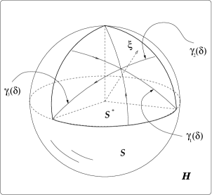
FIG. 1.: The family of Lesche’s critical distributions ($\alpha\!>\!1$). A statistical system can be represented by points ${\boldsymbol{\xi}}$ on a positive orthant ${\mathcal{S}}^{+}$ of the unit sphere ${\mathcal{S}}$ in a real Hilbert space ${\mathcal{H}}$. 1–parametric families of Leshe’s critical distributions are then represented by arcs ${\gamma}_{i}(\delta)=\left\{\xi_{k}(\delta)=\sqrt{\frac{~{}\delta\ \delta_{ik}}{2}+\left(1-\frac{\delta}{2}\right)\left(\frac{1-\ \delta_{ik}}{n-1}\right)};\;k\in 1,\ldots,n;\,\delta\in[0,2]\right\}$. Depicted example corresponds to ${\mathcal{S}}={\mathcal{S}}^{2}$.

We wish to ask whether some extension of (39) might have the non–zero measure. We will illustrate now that the answer is negative. In fact, we will show that with Bhattacharyya measure approaching $1$ (in the limit of large $n$) all distributions ${\mathcal{P}}\in{\mathbb{P}}_{n}$ inevitably fulfil Lesche’s condition (4). Inasmuch, all distributions which exhibit the critical behavior encountered in Ref. [12] have $\mu_{B}\rightarrow 0$ as $n\rightarrow\infty$. To prove this we employ the following isoperimetric inequality (also known as Levy’s lemma) [30]. Let $f$: ${\mathcal{S}}^{n-1}\mapsto{\mathbb{R}}$ be a $K$–Lipshitz function, i.e., for any pair ${\boldsymbol{\xi}}^{(1)}$, ${\boldsymbol{\xi}}^{(2)}\in{\mathcal{S}}^{n-1}$

$$||f({\boldsymbol{\xi}}^{(1)})-f({\boldsymbol{\xi}}^{(2)})||\leq K\ ||{\boldsymbol{\xi}}^{(1)}-{\boldsymbol{\xi}}^{(2)}||_{2}\,.$$ (69)

Then

$$\frac{V_{n-1}\left({\boldsymbol{\xi}}\in{\mathcal{S}}^{n-1};\ \left|f({\boldsymbol{\xi}})-\int_{{\mathcal{S}}^{n-1}}fd\mu\right|\ >\ C\right)}{V_{n-1}({\mathcal{S}}^{n-1})}\ \leq\ 4e^{-\vartheta C^{2}n/K}\,,$$ (70)

where $\mu$ is the Haar measure on ${\mathcal{S}}^{n-1}$ and $\vartheta$ is an absolute (i.e., $n$–independent) constant whose precise form is not important here .

Let us choose $f({\boldsymbol{\xi}})=||{\boldsymbol{\xi}}||_{2\alpha}$. Using the triangle inequality we have

$$\left|\ ||{\boldsymbol{\xi}}^{(1)}||_{2\alpha}-||{\boldsymbol{\xi}}^{(2)}||_{2\alpha}\right|\ \leq\ ||{\boldsymbol{\xi}}^{(1)}-{\boldsymbol{\xi}}^{(2)}||_{2\alpha}\ \leq\ ||{\boldsymbol{\xi}}^{(1)}-{\boldsymbol{\xi}}^{(2)}||_{2}\,,$$ (71)

so $||{\boldsymbol{\xi}}||_{2\alpha}$ is $1$–Lipshitz function. In addition,

$$||{\mathcal{P}}-{\mathcal{Q}}||_{1}=\sum_{i}\left|({\xi}^{(1)}_{i})^{2}-({\xi}^{(2)}_{i})^{2}\right|=\sum_{i}\left|\ {\xi}^{(1)}_{i}-{\xi}^{(2)}_{i}\right|\left({\xi}^{(1)}_{i}+{\xi}^{(2)}_{i}\right)\geq||{\boldsymbol{\xi}}^{(1)}-{\boldsymbol{\xi}}^{(2)}||^{2}_{2}\,.$$ (72)

So particularly when two distributions are $\delta$ close then their representative points on the sphere fulfil the inequality

$$\left|\ ||{\boldsymbol{\xi}}^{(1)}||_{2\alpha}-||{\boldsymbol{\xi}}^{(2)}||_{2\alpha}\right|\ \leq\ \sqrt{\delta}\,.$$ (73)

The next step is to calculate the mean $\int_{{\mathcal{S}}^{n-1}}f({\boldsymbol{\xi}})d\mu$. As it stands, this is quite difficult task but fortunately we may take advantage of the fact that

$$\int_{{\mathcal{S}}^{n-1}}\sum_{i}^{n}|\xi_{i}|^{2\alpha}d\mu({\boldsymbol{\xi}})\ = \ n\int_{{\mathcal{S}}^{n-1}}|\xi_{1}|^{2\alpha}d\mu({\boldsymbol{\xi}})\ =\ \frac{n\int_{0}^{\pi}|\cos(\theta)|^{2\alpha}(\sin(\theta))^{n-2}d\theta}{\int_{{\mathcal{S}}^{n-1}}(\sin(\theta))^{n-2}d\theta}$$ (74)

$$= \ \frac{n\Gamma(n/2)\Gamma(\alpha+1/2)}{\sqrt{\pi}\ \Gamma(n/2+\alpha)}\ \sim\ \frac{\Gamma(\alpha+1/2)2^{\alpha}}{\sqrt{\pi}}\ n^{1-\alpha}\,.$$ (75)

(Note that (75) is true for all $\alpha>0$. ) Using Jensen’s inequality we then have

$$E\left(||{\boldsymbol{\xi}}||_{2\alpha}\right)\ \equiv\ \int_{{\mathcal{S}}^{n-1}}||{\boldsymbol{\xi}}||_{2\alpha}d\mu\ \leq\ \sqrt[2\alpha]{\int_{{\mathcal{S}}^{n-1}}(||{\boldsymbol{\xi}}||_{2\alpha})^{2\alpha}d\mu}\ =\ \sqrt[2\alpha]{\frac{\Gamma(\alpha+1/2)2^{\alpha}}{\sqrt{\pi}}}\ n^{\frac{1}{2\alpha}-\frac{1}{2}}\,.$$ (76)

On the other hand, because all distributions from ${\mathbb{P}}_{n}$ fulfill the condition

$$n^{1-\alpha}\leq\sum_{i=1}^{n}p_{i}^{\alpha}\leq 1\,,\;\;\;\;\alpha\geq 1\,,$$ (77)

we have that $E\left(||{\boldsymbol{\xi}}||_{2\alpha}\right)\geq n^{\frac{1}{2\alpha}-\frac{1}{2}}$. Thus the mean value of $||{\boldsymbol{\xi}}||_{2\alpha}$ goes to zero as $b\left(n^{\frac{1}{2\alpha}-\frac{1}{2}}\right)$ where $b=b(n,\alpha)$ is some bounded function of $n$. Collecting results (75) and (76) together we can recast Levy’s lemma into form

$$\ \mu_{B}\left(\left|\ ||{\boldsymbol{\xi}}||_{2\alpha}-E\left(||{\boldsymbol{\xi}}||_{2\alpha}\right)\right|\,\leq\,C\right)\geq 1-4e^{-\vartheta C^{2}n}$$ (78)

$$\Rightarrow \ \mu_{B}\left(\left|||{\boldsymbol{\xi}}||_{2\alpha}-E\left(||{\boldsymbol{\xi}}||_{2\alpha}\right)\right|\leq\epsilon\left[E\left(||{\boldsymbol{\xi}}||_{2\alpha}\right)\right]^{p}\right)\ \geq\ 1-4\exp\left(-\vartheta\epsilon^{2}b^{2}n^{\left(1-p\left(\frac{\alpha-1}{\alpha}\right)\right)}\right)\,,$$ (79)

for some $\epsilon>0$. Note that due to symmetry of $f({\boldsymbol{\xi}})$ we were allowed to exchanged in (70) the averaging over the surface of ${\mathcal{S}}^{n-1}$ for the averaging over the positive octant $({\mathcal{S}}^{n-1})^{+}$. Result (79) implies that for any $\epsilon>0$ and any $1<p<\alpha/(\alpha-1)$ the inequalities

$$||{\boldsymbol{\xi}}||_{2\alpha}\ \geq\ E(||{\boldsymbol{\xi}}||_{2\alpha})\left(1-\epsilon\left[E\left(||{\boldsymbol{\xi}}||_{2\alpha}\right)\right]^{p-1}\right)\ \geq\ E\left(||{\boldsymbol{\xi}}||_{2\alpha}\right)e^{-2\epsilon\left[E\left(||{\boldsymbol{\xi}}||_{2\alpha}\right)\right]^{p-1}}\,,$$ (80)

$$||{\boldsymbol{\xi}}||_{2\alpha}\ \leq\ E(||{\boldsymbol{\xi}}||_{2\alpha})\left(1+\epsilon\left[E\left(||{\boldsymbol{\xi}}||_{2\alpha}\right)\right]^{p-1}\right)\ \leq\ E\left(||{\boldsymbol{\xi}}||_{2\alpha}\right)e^{\left[\epsilon E\left(||{\boldsymbol{\xi}}||_{2\alpha}\right)\right]^{p-1}}\,,$$ (81)

hold for almost all ${\boldsymbol{\xi}}\in{\mathbb{P}}_{n}$ (their Bhattacharyya measure is arbitrarily close to $1$ as $n$ increases). The fact that “well behaved” functions are at large $n$ practically constant on almost entire sphere is known as the concentration measure phenomenon [30, 31, 32]. In passing, the reader may notice that the relation (79) is a variant of Bernstein–Hoeffding’s large deviation inequality [31, 33].

Using now Minkowski’s triangle inequality

$$\left|||{\boldsymbol{\xi}}^{(1)}||_{2\alpha}-||{\boldsymbol{\xi}}^{(2)}||_{2\alpha}\right|\ \leq\ \left|||{\boldsymbol{\xi}}^{(1)}||_{2\alpha}-E(||{\boldsymbol{\xi}}||_{2\alpha})\right|+\left|||{\boldsymbol{\xi}}^{(2)}||_{2\alpha}-E(||{\boldsymbol{\xi}}||_{2\alpha})\right|\ \leq\ 2\epsilon\left[E\left(||{\boldsymbol{\xi}}||_{2\alpha}\right)\right]^{p}\,,$$

and bearing in mind (73) we can chose $\sqrt{\delta}\geq 2\epsilon\left[E\left(||{\boldsymbol{\xi}}||_{2\alpha}\right)\right]^{p}$. Consequently (for $n\geq 3$)

$$\frac{\left|{\mathcal{I}}_{\alpha}({\mathcal{P}})-{\mathcal{I}}_{\alpha}({\mathcal{Q}})\right|}{{\mathcal{I}}_{\alpha\ {\rm max}}} = \frac{2\alpha}{(\alpha-1)\log_{2}n}\left|\log_{2}\left(\frac{||{\boldsymbol{\xi}}^{(1)}||_{2\alpha}}{||{\boldsymbol{\xi}}^{(2)}||_{2\alpha}}\right)\right|\ \leq\ \frac{2\alpha}{(\alpha-1)}\left|\lg\left(\frac{e^{\epsilon\left[E\left(||{\boldsymbol{\xi}}||_{2\alpha}\right)\right]^{p-1}}}{e^{-2\epsilon\left[E\left(||{\boldsymbol{\xi}}||_{2\alpha}\right)\right]^{p-1}}}\right)\right|$$ (82)

$$= \frac{6\alpha\epsilon}{(\alpha-1)}\left[E\left(||{\boldsymbol{\xi}}||_{2\alpha}\right)\right]^{p-1}\ \leq\ \frac{6\alpha}{(\alpha-1)}\left(\frac{\delta}{4}\right)^{(p-1)/2p}\,.$$ (84)

Thus we see that one can always find an appropriate $\delta_{\varepsilon}$ for every $\varepsilon$, namely

$$\delta_{\varepsilon}\,\leq\,4\left(\frac{\varepsilon(\alpha-1)}{6\alpha}\right)^{2p/(p-1)}\,,$$ (85)

and so the observability condition (4) is satisfied in all cases for which inequalities (81) hold.

2 $\boldsymbol{0<\alpha<1}$ case

Similar analysis can be performed for critical distributions in the $\alpha<1$ case. The corresponding 1–parametric families of Lesche’s critical distributions are represented by arcs ${\varsigma}_{i}(\delta)=\left\{\xi_{k}(\delta)=\sqrt{\left(1-\frac{\delta}{2}\right)\delta_{ik}+\frac{\delta}{2}\left(\frac{1-\ \delta_{ik}}{n-1}\right)};\;k\in\hat{n};\,\delta\in[0,2]\right\}$. These arcs are identical with arcs $\gamma_{i}(\delta)$ depicted in Fig.1 only the orientation is reversed. Consequently the Bhattacharyya measure is again zero in this case.

We may now ask whether there exists some generalization of (42) such that the corresponding measure $\mu_{B}$ is non–zero. Answer is again negative. We show now that this is a consequence of the fact that almost all distributions ${\mathcal{P}}\in{\mathbb{P}}_{n}$ fulfill Lesche’s observability condition (4), while Bhattacharyya’s measure of those distributions which do not comply with the condition (4) tends to $0$ at large $n$.

To prove this we utilize once again Levy’s lemma. In this case we make identification $f({\boldsymbol{\xi}})=||{\boldsymbol{\xi}}^{(2)}||_{2\alpha}/E(||{\boldsymbol{\xi}}^{(2)}||_{2\alpha})$. Similarly as in the previous case we must determine first the asymptotic behavior of the mean $E\left(||{\boldsymbol{\xi}}||_{2\alpha}\right)$. This can be achieved by employing Jensen’s inequality

$$\sqrt[2\alpha]{\frac{\Gamma(\alpha+1/2)2^{\alpha}}{\sqrt{\pi}}}\ n^{\frac{1}{2\alpha}-\frac{1}{2}}=\sqrt[2\alpha]{\int_{{\mathcal{S}}^{n-1}}(||{\boldsymbol{\xi}}||_{2\alpha})^{2\alpha}d\mu}\ \leq\ \int_{{\mathcal{S}}^{n-1}}||{\boldsymbol{\xi}}||_{2\alpha}d\mu\,,$$ (86)

together with inequality

$$1\leq\sum_{i=1}^{n}p_{i}^{\alpha}\leq n^{1-\alpha}\,,\;\;\;0<\alpha<1\,.$$ (87)

Therefore $E\left(||{\boldsymbol{\xi}}||_{2\alpha}\right)$ is unbounded at large $n$ and it approaches infinity as $a(n^{\frac{1}{2\alpha}-\frac{1}{2}})$ ($a=a(n,\alpha)$ is some function with lower and upper bound in $n$). Employing now the estimate:

$$\left|\ ||{\boldsymbol{\xi}}^{(1)}||_{2\alpha}-||{\boldsymbol{\xi}}^{(2)}||_{2\alpha}\right|\leq||{\boldsymbol{\xi}}^{(1)}-{\boldsymbol{\xi}}^{(2)}||_{2\alpha}\leq||{\boldsymbol{\xi}}^{(1)}-{\boldsymbol{\xi}}^{(2)}||_{2}\ n^{\frac{1}{2\alpha}-\frac{1}{2}}\leq\sqrt{\delta}\ n^{\frac{1}{2\alpha}-\frac{1}{2}}\,,$$ (88)

(where the triangle and Hölder inequalities were successively applied) we obtain that $f({\boldsymbol{\xi}})$ is $1/\underline{a}$–Lipshitz. Here $\underline{a}$ is the lower bound of $a$. Levy’s lemma then implies that

$$\mu_{B}\left(\left|\frac{||{\boldsymbol{\xi}}||_{2\alpha}}{E\left(||{\boldsymbol{\xi}}||_{2\alpha}\right)}-1\right|\leq\ \epsilon\right)\ \geq\ 1-4e^{-\vartheta\underline{a}\epsilon^{2}n}\,,$$ (89)

for any $\epsilon>0$. Result (89) suggests that for a sufficiently small $\epsilon$ ($\epsilon\leq 1,59\ldots$) the inequality

$$e^{-2\epsilon}\leq\ 1-\epsilon\ \leq\ \frac{||{\boldsymbol{\xi}}||_{2\alpha}}{E(||{\boldsymbol{\xi}}||_{2\alpha})}\ \leq\ 1+\epsilon\ \leq\ e^{\epsilon}\,,$$ (90)

holds for almost all ${\boldsymbol{\xi}}\in{\mathbb{P}}_{n}$ ($\mu_{B}\rightarrow 1$ as $n\rightarrow\infty$). So we again encounter the concentration of measure phenomenon - at large $n$ almost all Bhattacharyya measure is concentrated on ${\boldsymbol{\xi}}$’s fulfilling the condition $||{\boldsymbol{\xi}}||_{2\alpha}\approx E(||{\boldsymbol{\xi}}||_{2\alpha})$. Using now

$$\left|\frac{||{\boldsymbol{\xi}}^{(1)}||_{2\alpha}}{E(||{\boldsymbol{\xi}}||_{2\alpha})}-\frac{||{\boldsymbol{\xi}}^{(2)}||_{2\alpha}}{E(||{\boldsymbol{\xi}}||_{2\alpha})}\right|\ \leq\ \left|\frac{||{\boldsymbol{\xi}}^{(1)}||_{2\alpha}}{E(||{\boldsymbol{\xi}}||_{2\alpha})}-1\right|+\left|\frac{||{\boldsymbol{\xi}}^{(2)}||_{2\alpha}}{E(||{\boldsymbol{\xi}}||_{2\alpha})}-1\right|\ \leq\ 2\epsilon\,,$$ (91)

and bearing in mind (88) we can set $\delta=4\epsilon^{2}\underline{a}^{2}$. Consequently (for $n\geq 3$)

$$\frac{\left|{\mathcal{I}}_{\alpha}({\mathcal{P}})-{\mathcal{I}}_{\alpha}({\mathcal{Q}})\right|}{{\mathcal{I}}_{\alpha\ {\rm max}}} = \frac{2\alpha}{(1-\alpha)\log_{2}n}\left|\log_{2}\left(\frac{||{\boldsymbol{\xi}}^{(1)}||_{2\alpha}}{||{\boldsymbol{\xi}}^{(2)}||_{2\alpha}}\right)\right|\ \leq\ \frac{2\alpha}{(1-\alpha)\lg n}\left|\lg\left(\frac{e^{\epsilon}}{e^{-2\epsilon}}\right)\right|$$ (92)

$$= \ \frac{6\epsilon\alpha}{(1-\alpha)\lg n}\ \leq\ \frac{3\sqrt{\delta}\alpha}{(1-\alpha)\underline{a}}\,.$$ (93)

As in the previous case we can conclude that it is always possible to find an appropriate $\delta_{\varepsilon}$ for every $\varepsilon$, namely

$$\delta_{\varepsilon}\,\leq\,\left(\frac{\underline{a}(1-\alpha)\varepsilon}{3\alpha}\right)^{2}\,.$$ (94)

So the observability condition (4) is satisfied in all cases for which (90) holds. In passing we should mention that the underlying reason behind the relations (79) and (89) lies in the fact that $n$-spheres ${\mathcal{S}}^{n}$ equipped with the Bhattacharyya distance $\phi_{n}$ and Haar measure $\mu_{n}$ form the so called normal Levy family [30, 34]. In can be shown [30] that the concentration measure phenomenon is an inherent property of any Levy family.

The moral of this section can be summarized in the following way: whenever one selects as the state space for Rényi entropies the space of all discrete statistics then a non–uniform continuity behavior (i.e., violation of Lesche’s condition (4)) can be observed for a certain set of distribution functions in the limit of large $n$. We demonstrated that the cardinality of such critical distributions is of zero Bhattacharyya measure in the space of all $n\rightarrow\infty$ probability distributions. One may relate those zero measure distributions to the so called $l_{\alpha}$–bounded distributions (i.e., distributions whose $l_{\alpha}$ norm has non–zero lower bound for $\alpha>1$ and a finite upper bound for $\alpha<1$). This can be plainly seen from the fact that for $l_{\alpha}$–bounded distributions the critical conditions (75) and (90) cannot be satisfied.

V Observability of Rényi entropies: Continuous probability distributions and multifractals

Let us briefly illustrate here that the conditions of absolutely continuous PDF’s or multifractality are themselves sufficiently restrictive to ensure that the instabilities discussed in the previous section do not occur. To see this let us consider Eqs.(11) and (17). The latter imply that for any ${\mathcal{P}}_{n}$ and ${\mathcal{P}}_{n}^{\prime}$ for which the renormalized Rényi entropy exists the following identity holds

(95)

$$\frac{|{\mathcal{I}}_{\alpha}({\mathcal{P}}_{n})-{\mathcal{I}}_{\alpha}({\mathcal{P}}_{n}^{\prime})|}{{\mathcal{I}}_{\alpha\;\rm{max}}} = \frac{|-D(\alpha)\log_{2}l+{\mathcal{I}}^{r}_{\alpha}+D(\alpha)\log_{2}l-{{\mathcal{I}}^{r}_{\alpha}}^{\prime}+o(1)|}{D(\alpha)\log_{2}(1/l)}$$ (96)

$$= \frac{|{\mathcal{I}}^{r}_{\alpha}-{{\mathcal{I}}^{r}_{\alpha}}^{\prime}|}{D(\alpha)\log_{2}(1/l)}+o(1)\,.$$ (97)

Superscript $r$ denotes renormalized quantities. Note particularly that ${\mathcal{I}}_{\alpha}^{r}$ are by construction finite and $n$ (i.e., $l$) independent. Using the fact that $\lg x\leq(x-1)$ together with Hölder inequality and Eq.(72) we have for two $\delta$–close distributions

$$|{\mathcal{I}}_{\alpha}({\mathcal{P}}_{n})-{\mathcal{I}}_{\alpha}({\mathcal{P}}_{n}^{\prime})|\ \leq\ \frac{2\alpha k}{|1-\alpha|}\frac{\left|||{\boldsymbol{\xi}}^{(1)}||_{2\alpha}-||{\boldsymbol{\xi}}^{(2)}||_{2\alpha}\right|}{\min(||{\boldsymbol{\xi}}||_{2\alpha})}\ \leq\ \frac{2\alpha k}{|1-\alpha|}\ \frac{\max(||{\boldsymbol{\xi}}||_{2\alpha})}{\min(||{\boldsymbol{\xi}}||_{2\alpha})}\ \sqrt{\delta}\,,$$ (98)

with $k=1/\lg 2$. Realizing that (11) and (17) imply

$$||{\boldsymbol{\xi}}||_{2\alpha}=e^{\frac{(1-\alpha)}{2\alpha}\left(-D(\alpha)\log_{2}l+{\mathcal{I}}^{r}_{\alpha}+o(1)\right)}\,,$$ (99)

we can straightforwardly write that

$$|{\mathcal{I}}^{r}_{\alpha}-{{\mathcal{I}}^{r}_{\alpha}}^{\prime}|+o(1)\ \leq\ \frac{2\alpha k}{|1-\alpha|}\ \sqrt{\delta}\ e^{\frac{(1-\alpha)}{2\alpha}|({\mathcal{I}}^{r}_{\alpha})_{\rm{max}}-({\mathcal{I}}^{r}_{\alpha})_{\rm{min}}|+o(1)}\ \equiv\ \frac{2\alpha k}{|1-\alpha|}\ {\mathcal{B}}\sqrt{\delta}\,.$$ (100)

Here ${\mathcal{B}}$ is an absolute constant representing the upper bound for the exponential. Gathering results (97) and (100) together we can finally write (for $n\geq 2$)

$$\frac{|{\mathcal{I}}_{\alpha}({\mathcal{P}}_{n})-{\mathcal{I}}_{\alpha}({\mathcal{P}}_{n}^{\prime})|}{{\mathcal{I}}_{\alpha\;\rm{max}}}\ \leq\ |{\mathcal{I}}^{r}_{\alpha}-{{\mathcal{I}}^{r}_{\alpha}}^{\prime}|+o(1)\ \leq\ \frac{2\alpha k}{|1-\alpha|}\ {\mathcal{B}}\sqrt{\delta}\,.$$ (101)

It is then clear in this case that one can easily find an appropriate $\delta_{\varepsilon}$ for every $\varepsilon$, namely

$$\delta_{\varepsilon}\ \leq\ \left(\frac{\varepsilon(1-\alpha)}{2\alpha k{\mathcal{B}}}\right)^{2}\,.$$ (102)

represents a correct choice. So for all pairs ${\mathcal{P}}_{n}$ and ${\mathcal{P}}_{n}^{\prime}$ which lead in $n\longrightarrow\infty$ limit to continuous PDF’s (or multifractals) the Leshe condition (4) applies. It is therefore the very definition of systems with absolutely continuous PDF’s/ multifractals (incorporated in Eqs.(9) and (15)) that naturally avoids the situations with instability points confronted in the previous section.

VI Conclusions

In this paper we have attempted to make sense of the recent claims concerning a total non–observability of Rényi’s entropy. We have found that problems have arisen from uncritical use of Lesche’s observability criterion. We have proved that the latter criterion, as it stands, does not rule out observability of Rényi entropies in large class of systems. Systems with finite number of microstates or multifractals being examples. This is so because the structure of the space of distribution functions (or PDF’s) over which such systems operate essentially prohibits an existence of “critical” situations considered by Lesche. In cases where such situations are encountered, namely in systems with (countable) infinity of microstates, we argue that Lesche’s uniform continuity condition is too tight to serve as a decisive criterion for the observability.

In previous works the uniform continuity condition was used to force observability upon state functions. As we have shown, it is not just unnecessary to do this but it also causes the Lesche criterion to produce incorrect results in certain cases. By identifying the probability distribution with a state variable this has led to confusion about the observability of Rényi’s entropy. Once the uniform continuity condition is dropped, we can clear up these confusing points. For this purpose we present a more intuitive concept of observability by allowing the quantity in question to have a certain amount of “critical” points provided that the cardinality of the critical points in the state space is of zero measure.

It is definitely interesting to know what the “critical regions” correspond to. In case of Rényi entropies we offer a partial reply to this question. Namely, for systems with (countable) infinity of microstates we show that the critical regions correspond to the $\delta$–vicinity of $l_{\alpha}$–bounded distributions. Basically such distributions correspond to (ultra)rare events which are frequently encountered e.g., in particle detection (double beta or tritium decays being examples). We have proved that the Bhattacharyya measure of these distributions must be zero. As $l_{\alpha}$–bounded distributions are not existent in (coarse–grained) multifractals or in systems with continuous PDF’s, neither in systems at thermal equilibrium, there is no a priori reason to disregard Rényi entropies as observable in the aforementioned instances. On the other hand, it is known that many systems undergo “statistics transitions” (stockmarket bidding and continuous phase transitions with their exponential–law - power–law distribution “transitions” may serve as examples). It might be also expected that in dynamical systems away from equilibrium transitions to $l_{\alpha}$–bounded statistics may play a relevant rôle. In any case, one can turn the sensitivity of Rényi entropies to a virtue as it could be used as a diagnostic instrument for an analysis of (ultra)rare–event systems, similarly as, for instance, temperature sensitivity of the susceptibility is used as a diagnostic tool in continuous phase transitions. We believe that further investigation in this direction would be of a great value.

Let us finally stress that there is also a conceptual reason why the observability à la Lesche should be viewed with some hint of scepticism. This is because the observability treated in such a framework is not a unique concept. Indeed, Lesche’s condition can brand a quantity as observable under one choice of state variables and as non–observable under a different choice, even if two such choices overlap in the scope of physical situations they describe. Typical example is the Gibbs–Shannon entropy. Here, according to the above criterion, the entropy is observable if the probability distribution is chosen as the state variable [13, 12]. On the other hand, if temperature and pressure are state variables then entropy develops discontinuity in any system which undergoes first order phase transition (Clausius–Clapeyron equation) and hence it is not for such systems uniformly continuous function of state variables, and according to (1) (or (2)) it is doomed to be non–observable. In this connection it is interesting to notice that because the parameter $\alpha$ plays formally rôle of inverse temperature [22, 35] one may expect that various limits may not commute similarly as in Gibbsian statistical physics. Namely, we may anticipate that $\lim_{\alpha\rightarrow 1}\lim_{n\rightarrow\infty}\neq\lim_{n\rightarrow\infty}\lim_{\alpha\rightarrow 1}$. In fact, Lesche [12] and other authors [13] applied the sequence of limits $\lim_{n\rightarrow\infty}\lim_{\alpha\rightarrow 1}$. In such a case they concluded that Rényi entropy of order one (Shannon’s entropy) is observable while the rest of Rényi entropies is not (despite the fact that Rényi entropies are analytic in $\alpha\in{\mathbb{R}}^{+}$, see Ref. [20]). On the other hand, when one utilizes the “thermodynamical” order, i.e., $\lim_{\alpha\rightarrow 1}\lim_{n\rightarrow\infty}$, then also Rényi’s entropy of order one develops instability points (this may be easily checked by noticing that unobservability argument presented in [12] is continuous in $\alpha=1$). The latter seems to support our previous comment that Shannon’s entropy should not be uniformly continuous in the space of discrete distribution functions in order to account, for instance, for the first–order phase transitions.

References

References

- [1] C. Caratheodory, Math. Ann. 67 (1909) 355; H.A. Buchdahl, Am. J. Phys. 17 (1949) 212.
- [2] R. Balian, From Microphysics to Macrophysics, Methods and Applications of Statistical Physics, Vol.1 (Springer–Verlag, Heidelberg, 1991).
- [3] A.I. Khinchin, Mathematical Foundations of Statistical Mechanics (Dover Publications, Inc., New York, 1949).
- [4] A. Rényi, Probability Theory (North-Holland, Amsterdam, 1970); Selected Papers of Alfred Rényi, Vol.2 (Akadémia Kiado, Budapest, 1976).
- [5] P. Jizba, cond-mat/0301343.
- [6] C. Tsallis, J. Stat. Phys. 52 (1988) 479; J.H. Havrda and F. Charvat, Kybernatica 3 (1967) 30.
- [7] http://astrosun.tn.cornell.edu/staff/loredo/bayes/
- [8] A. Bialas and W. Czyz, Acta Phys. Pol. B31 (2000) 2803; Phys. Rev. D61 (2000) 74021; M.K. Suleymanov, M. Sumbera, I. Zborovsky, hep-ph/0304206 .
- [9] C. Essex, C. Schultzky, A. Franz and K.H. Hoffmann, Physica A 284 (2000) 299.
- [10] T.C. Halsey, M.H. Jensen, L.P. Kadanoff, I. Procaccia and B.I. Shraiman, Phys. Rev. A 33 (1986) 1141; M.H. Jensen, L.P. Kadanoff, A. Libchaber, I. Procaccia and J. Stavans, Phys. Rev. Lett. 55 (1985) 2798; K. Tomita, H. Hata, T. Horita, H. Mori and T. Morita, Prog. Theor. Phys. 80 (1988) 963; H.G.E. Hentschel and I. Procaccia, Physica D 8 (1983) 435.
- [11] S. Abe and Y. Okamoto (Eds.), Nonextensive Statistical Mechanics and Its Applications (Springer–Verlag, New York, 2001).
- [12] B. Lesche, J. Stat. Phys. 27 (1982) 419.
- [13] S. Abe, Phys. Rev.E66(2002) 046134
- [14] C. Cachin, Entropy Measures and Unconditional Security in Cryptography, PhD thesis, ETH Zurich, May 1997; ftp://ftp.inf.ethz.ch/pub/publications/dissertations/th12187.ps.gz .
- [15] D. Harte, Multifractals Theory and Applications, (Chapman & Hall/CRC, New York, 2001); M.B. Geilikman, T.V. Golubeva and V.F. Pisarenko, Earth & Plan. Sci. Let. 99 (1990) 127.
- [16] H. Maassen and J.B.M. Uffink, Phys. Rev. Lett. 60 (1988) 1103.
- [17] see e.g., W. Rudin, Functional Analysis, (McGraw-Hill Companies, New York, 1991).
- [18] see e.g, F. Berthier,J.-P. Diard, L. Pronzato, Automatica 35 (1999) 1605.
- [19] see e.g., E.D. Sontag and Y. Wang, Systems Control Lett. 29(1997) 279.
- [20] P. Jizba and T. Arimitsu, cond–mat/0207707 .
- [21] L.L. Campbell, Information and Control, Vol.8 (1965) 423.
- [22] H. Sakaguchi, Prog. Theor. Phys. 81 (1989) 732.
- [23] J. Feder, Fractals (Plenum Press, New York, 1988).
- [24] S. Kullback and R. Leibler, Ann. Math. Statist. 22(1951) 79.
- [25] T. Arimitsu and N. Arimitsu, Physica A 295 (2001) 177; J. Phys. A: Math. Gen. 33 (2000) L235 [CORRIGENDUM: 34 (2001) 673]; Physica A 305 (2002) 218; J. Phys.: Condens. Matter 14 (2002) 2237; cond-mat/0306042 .
- [26] A. Bhattacharyya, Bull. Calcutta Math. Soc. 35 (1943) 99; D.C. Brody and L.P. Hughston, Proc. R. Soc. London A457 (2001) 1343.
- [27] N.Thacker, F.J.Aherne and P.I.Rockett, Kybernetika, 34 (1997) 363; D.C.Brody and L.P.Hughston, in Disordered and Complex Systems, (p. 281-288) P.Sollich, A.C.C.Coolen, L.P.Hughston, Eds. AIP Press, NY (2000); S.S.Dragomir, math.PR/0304240.
- [28] W.K.Wootters Phys. Rev. D23 (1981) 357; H.Araki and G.Raggio, Lett. Math.Phys. 6 (1982) 237; D.C.Brody and L.P.Hughston, Phys.Rev.Lett. 77 (1996) 2851; D.C.Brody and L.P.Hughston, Proc. R. Soc. Lond. A454 (1998) 2445.
- [29] K.Kukunaga, Introduction to Statistical pattern Recognition, (Academic Press, Inc., NY, 1990); R.O.Duda, P.E.Hart, D.G.Stork, Pattern Classification (Wiley, London, 2000); T.Kailath, IEEE Trans.Comm.Theory 15 (1967) 52.
- [30] V.D. Milman, G. Schechtman, Asymptotic Theory of Finite Dimensional Normed Spaces (Spring–verlag, New York, 1980).
- [31] K.M. Ball, An elementary introduction to modern convex geometry, Flavors of Geometry, Ed. by Silvio Levy, (Cambridge University Press, New York, 1997).
- [32] R.J. Gardner, Bulletin of the American Mathematical Society, 39 (2002) 355.
- [33] D. Williams, Probability with martingales (Cambridge University Press, Cambride, 1991).
- [34] M. Ledoux, Concentration of measure and logarithmic Sobolev inequalities, ed. by J. Azéma, M. Émery, M. Ledoux and M. Yor, Lecture Notes in Mathematics 1709 (Springer, Berlin, 1999).
- [35] P. Jizba and T. Arimitsu, AIP Conf. Proc. 597 (2001) 341.