Self-Organized Criticality as a Phase Transition

The original sandpile model of Bak, Tang and Wiesenfeld from 1987 has inspired lots of consequent work and further ideas of how to describe the birth of scale-invariant statistics in various systems and in particular models. In this article the basic ingredients of self-organized criticality (SOC) are overviewed. In line with the orginal arguments of BTW SOC is now known to be a property of systems where dissipation and external drive maintain a delicate balance. The qualitative and quantitive understanding of the SOC state and deviations from it can thus be addressed, by mapping the typical cellular automata exhibiting SOC to theories, that in fact describe critical extended systems as such. Currently two such approaches are known, based on the connections of SOC to variants of absorbing state phase transitions and the physics of elastic manifolds or interfaces in random media. These are reviewed and discussed. Finally, some open theoretical problems and experimental suggestions are outlined.

1 Introduction

Usually statistical physics is on the textbook level a subject that deals with “boring” properties of matter and the associated basic thermodynamic quantities. There is however a modern challenge to this, that attempts to deal with all kinds of phenomena with statistical physics tools. One of the simple reasons is the discovery of many (effective) power-laws or “fractals”, in the statistics of measurable quantities. This implies that within the appropriate window the system is scale-invariant, which in the language of statistical mechanics brings us to the field of phase transitions. The next question that follows is then: how come so many phenomena have parameters finely tuned to the point where the equations and laws governing them allow for “criticality”? Consider the prototypical two-dimensional Ising model as a example: for sure one needs to tune the temperature to $T_{c}$ to reach the same effect.

The seminal papers of Bak, Tang and Wiesenfeld (BTW) started a literal avalanche in this respect. They coined the term of “Self-Organized Criticality” (SOC), with an associated set of claims, conjectures, results, and a simple model well within grasp of anyone fluent with computers. The main idea of BTW was that such a sandpile mode would be effective in explaining the presence of $1/f$ -noise in Nature, a prototypical example of power-laws indeed. The purpose of this article is to give an overview of where the mainstream SOC understanding has lead to, from the starting point of the 1987-1988 BTW publications [1]. For this goal it is instructive to start with the original BTW sandpile model, for a brief look as to what the rules and aspects of the SOC sandpiles imply. These are often most defined as cellular automata, on hypercubic lattices of size $L^{d}$ . The original BTW numerical results concentrated on $d=2$. Each site $x$ has $z(x,t)$ grains. There are two crucial ingredients that define the dynamics in the BTW model. When $z(x,t)$ exceeds a critical threshold $z_{c}$ (a constant, here 3), the site is active and topples. The grains (4 in the $2d$ BTW example) are removed from x and given to the nearest neighbors (nn). The effect of this rule is to create a non-linearity: in the absence of any activity in the nn’s of x the site stays quiescent, forever if $z_{x}\equiv z(x,t)<z_{c}$ . In other words, the BTW model has $z_{c}$ equal to a constant, $z_{c}=2d-1$, and the toppling rule:

$$z(x,t+1)=z(x,t)-2d$$ (1)

$$z(y,t+1)=z(y,t)+1$$ (2)

where $y$ denotes all the $2d$ nearest neighbors of the site $x$.

One may now study two fundamental limits (note that clearly other scenarios can be envisioned). Either one prepares the system with a fixed number of grains $n_{tot}=\sum_{x}z_{x}$ , and observes what happens, with e.g. periodic boundary conditions. Due to the presence of the nonlinearity it is easy to see that there are two opposite limits, an absorbing state where all $z_{x}<z_{c}$ and nothing happens, and a state of eternal activity where for all $t$ for some $x$ $z_{x}>z_{c}$ . This defines a “fixed energy ensemble” (FES) as it has been denoted in the literature. Clearly there has to be a (phase) transition as n tot is varied between the two extremes.

However, the particular case of “original” SOC of BTW is created by different conditions. What one wants to obtain is a steady state. This is obtained by combining open boundary conditions that are balanced with a “drive”. The boundaries are chosen to be such that the grains which ”topple” out of the system are lost, simply. Eg. in $2d$ a site which touches the boundary loses a grain out of the four it gives out. The SOC state is now obtained by using a modern version of Maxwell’s demon: if and only if there are no active sites ($z_{x}>z_{c}$) one grain is added to a randomly chosen site $x$: $z(x,t)\rightarrow z(x,t)+1$. Except for the presence thereof there is no “tuning” whatsoever. Clearly, the effect of an added grain is either to build up $z_{x}$ or to launch an avalanche if x is “marginally stable” if $z_{x}=z_{c}$ . The original claim of BTW was that the sizes of avalanches - measured as the number of times that any single site would get active after a single grain addition - would follow a power-law, as would the duration (multiple simultaneous topplings being allows) and the area or support on the $L^{d}$ lattice,

$$f(s)\simeq s^{-\tau_{s}}f(s/s_{c}),$$ (3)

with the avalanche size exponent $\tau_{s}$ and the cut-off dimension $s_{c}=L^{D_{s}}$ . The scaling function $f$ expresses the fact that avalanches are limited by the scale $s_{c}$ and thus decays quickly beyond that. Thus there would be a subtle balance of driving and dissipation in a SOC system, with power-laws arising apparently without any fine-tuning and hence the birth of the acronym.

The essence of SOC as from the BTW model is thus non-linearity and a combination of dissipation and driving [2]. There is an easy set of questions that follows immediately, in particular from the analogies with other phase transitions:

• universality: what kind of exponents ($\tau_{s}$ , $D_{s}$ etc.) would one be able to obtain depending on the particular details of the model?

• what does SOC “mean” in fact?

• how broad is this paradigm in terms of applicability?

• what is the right “continuum theory” for SOC?

In the rest of this article the status of the two ideas and the follow-up questions will be examined, in the light of recent progress on mapping SOC sandpiles to other systems. In this, the main emphasis is on analogies with interface depinning and absorbing state phase transitions. Both these allow to adapt to the ensembles (SOC, FES) in which the simple SOC automata are run, and moreover present the essential feature of a “nonlinearity”, of a threshold element as we will see below. These present two different “generic” types of continuum limits. For the second one, we have as the dynamical variable the activity, $\rho({\bf x},t)$. The interface depinning variants of SOC boil down in most effective form as a variable $H({\bf x},t)\equiv\int^{t}\rho({\bf x},t)d\tau$ and its dynamical equation $\partial_{t}H({\bf x},t)\dots$. The picture of SOC is completely equivalent as to how the right ensemble is created. This will be highlighted with examples in the next section.

1.1 Theoretical aspecs of sandpiles

Analogies with other systems in statistical mechanics have been around for a long while but have not been exhausted even by now. Tang and Bak already noted that one can perturb - on the cellular automaton level - sandpiles by driving them at a steady, slow rate so that overlapping avalanches are not too frequent. They also conjectured - based on ideas from equilibrium phase transitions - several exponent relations, to describe the correlation length and the correlation time in the proximity of the vanishing drive rate, and most importantly identified a (correct) order parameter, the average activity or probability that a site is active ($z_{x}>z_{c}$ in the BTW case). The mean-field treatment results in the exponents of the contact process or directed percolation (DP) [3], and hence it immediately brings to the question whether sandpiles are just an example of an absorbing state phase transition like DP.

For the BTW model, again, Narayan and Middleton noted that it can be obtained from a discrete version of an equation describing charge-density waves (not surprising considering the history of the model as such) [4]. This equation is known another contexts and with a different noise term as the quenched Edwards-Wilkinson equation (QEW). It describes the dynamics of a forced domain wall in a random magnet. The impurities pin the interface and a driving force counteracts the pinning. Later, Paczuski and Bottcher pointed out that a particular “rice pile” SOC model [5] could be mapped also into the same system.

The presence of these two analogies (see also [6, 7]) or in more concrete terms mappings to (continuum) systems from SOC [8, 9] makes it possible to identify firmly many answers to the above mentioned problems, and in general to understand the critical properties without any conceptual confusions. These are discussed, in combination with the missing pieces of the puzzle, in the later paragraphs. As will become clear the nature of SOC in such typical cellular automata is a particular ensemble version of various non-equilibrium phase transitions. In many of the early papers analogies were drawn with the physics of equilibrium ones. Here, however, the situation is different and one for instance is not necessarily able to define a free energy for the system, or even a Hamiltonian (e.g. the perennial Kardar-Parisi-Zhang problem serves as an example [10]). It also becomes more evident what the correct renormalization group procedure is, in contrast to various real-space, mean-field and other attempts [11, 12, 13, 14]. This leads to an understanding of where the differences in the numerically found scaling behavior among the BTW, Manna [15], Zhang [16] etc. models originate from.

In most cases it is also obvious that the SOC state is indeed achieved only in a particular point of the phase space, the only reason why this is not obvious to begin with is that it becomes apparent after such connections to other models are made clear. Thus in general there is no “generic scale invariance” [17, 18] unless one goes one step further: in the driven interface paradigm the system still exhibits critical fluctuations off the SOC state, but the character of the fluctuations changes. The simple analogy here is the thermalization of the noise in a depinning problem, and the changed interface fluctuations. Here one has to be careful about the ensemble that is perturbed off the critical point: in translation-invariant models with a uniform dissipation rate $\epsilon$ one can observe avalanches when $\epsilon\rightarrow 0^{+}$ [13, 14] similarly to the SOC ensemble. This is of course true only when the drive rate $h$ is adjusted so that $h/\epsilon\rightarrow 0$ [17, 19, 14], ie. in the limit that these two very slow scales are still “infinitely separate” [17]. If one accepts the idea that SOC actually arises from “normal criticality” by some clever mechanism (e.g. “sweeping the instability” as was proposed [20]), then the question still remains how this can be made to work, and in e.g. the interface picture this becomes immediately obvious.

The original BTW model itself still attracts interest since it does have a powerful Abelian symmetry, peculiar of a discrete cellular automaton. As shown by Dhar, Priezzhev and co-workers in a series of papers there are connections to spanning trees on lattices [21, 22], thus to the critical $q=1$ Potts model (and in $2d$ to conformal invariance) [23]. In this respect it has however lost the aura of generality that the original papers advocated, not forgetting the long-standing controversies about the various universality classes of SOC models - related to the numerically determined exponents based on Eq. (3). Recent numerical studies have even pointed out that the BTW model shows multiscaling: the avalanches exhibit a full spectrum of scales, whose origins are not understood [24]. Such numerical studies have made it apparent that there are definately different universality classes, as the connections to interface depinning and APT’s should make clear below.

In the following models that involve strict “extremal dynamics”, in the sprit of the Bak-Sneppen model [25], are excluded. The idea here is that one (in the interface context) advances the site which has the largest local force. Clearly this kind of dynamical mechanism is just another version of the demon inside the BTW sandpile, an even smarter one since he has now to know the state of the system in greater detail. We shall also not discuss the so-called forest-fire models [26, 27], that have the difference that one has three states for a site: empty, a living tree, and a burning one. For this class one has no such conservation law as exemplified by the Laplacian of the interface equation or by the energy field of the APT class with conservation. It is an open question how to find similar connections to continuum models. We also omit directed models which as such are often more simple to understand theoretically.

1.2 Experimental signatures of SOC

The obvious question to ask is, what is the quantity to measure given that SOC is in fact a “usual phase transition”? There are two answers: either one is concerned with avalanche behavior, like in a typical sandpile model, or then one is interested in some quantity that would be able e.g. to establish whether the dynamics are indeed governed by or close to something akin a SOC critical point. Given the fact that one needs a separation of timescales it becomes clear that sandpile-like behavior is not easy to conjure in an experiment. On the other hand, it is clear that a generic phenomenon like $1/f$-noise is precisely speaking far from the typical SOC manifestations.

Laboratory-scale experiments for this purpose were attempted soon after the first BTW papers inspired by the “sandpile” idea [28]. Unfortunately, there is little reason as to why a real sandpile should behave like a cellular automaton. In particular, the flow of grains once started involves inertia [29]. The ingenuity of experimentalists then lead (in Oslo) to the discovery that one can simply substitute with (elongated) rice grains, and a power-law avalanche distribution follows [30] (see also [31]).

In essence, to mimick sandpiles one thus needs diffusive motion of the “particles”, ie. the equation of motion has to contain precisely the same ingredients of a threshold and overdamped motion once that is exceeded. Such conditions are provided by domain walls (DW) in ferromagnets - as we will see one can easily define a sandpile that describes the dynamics of a DW - and vortices in type-II superconductors. The former can be observed by e.g. optical means or by the noise produced by domain wall motion, known as the Barkhausen effect [32]. It is possible to observe avalanches, with a size distribution that extends as a power-law over more than three decades [33, 34, 35, 36, 37]. The classical Barkhausen DW experiment corresponds however to the slowly driven, translationally invariant case outlined above (and not to the SOC ensemble): a constant external field ramp corresponds to a constant velocity for the driven DW.

The recipe for superconductors is to increase the external field which pushes vortices or flux lines into a sample (recall of type II). The Bean state [38, 39] that ensues has a conservation law (vortices), and can be controlled with the rate of increase of the external field. One can observe avalanches, exhibiting power-law behavior [40, 41, 42]. Indeed there are sandpile models to describe such behavior [43], and on the other hand coarse-grained lattice models that are close to sandpiles in spirit [44] (to say nothing about more complicated simulations [45]). In both these cases the actual role of SOC in the phenomena at hand seems slightly secondary, however.

Avalanches have also been observed in a more promising field from the point of view of potential applications: fracture and plasticity. While there is lots of evidence (in terms of acoustic emission, the energy relased by microscopic events) for the existence of power-laws both in laboratory experiments [46, 47, 48] and in earthquakes, it is not clear at all how much these have to do with SOC. In failure of brittle materials it is clear that the underlying processes are irreversible and have nothing in common with the basic premises of a SOC state. In the case of earth-quakes the scales involved are such that it may seem more prudent to explain eg. the classical Richter’s and Omori’s laws (of magnitudes and aftershock intervals) via a suitable SOC model. However, no direct connection has been established so far [49]. Plasticity and dislocation dynamics seem better in this respect, as a field of application of SOC ideas (see [50, 51] for AE evidence). One has the possiblity of a steady-state and the system can be driven by slowly applied external strain.

Perhaps the most enticing field where SOC concepts have been utilized is plasma and space physics. The crucial ingredients here are the presence of non-linearities (given by the character of e.g. the magnetohydrodynamic equations that can be proposed for the Earth’s magnetotail sheet), external drive (ionospheric activity vs. solar wind, or the solar flares vs. sun’s heating), and spatial inhomogeneity in that the dissipation and drive do not necessarily take place uniformly. Both in space and laboratory plasmas one can obtain measured statistics (like the particle flux driven by the nonlinear transport at the plasma edge in a fusion device, or the magnetospheric AE index) that can be then analyzed in terms of SOC characteristics. Several reviews exist that outline the subject (whether one is interested in fusion or space aspects) [52, 53, 54, 55, 56, 57]. There is clear evidence of power-laws in eg. the waiting times of avalanches and energy dissipated [53]. In these contexts some of the differences to usual sandpile models are based e.g. on comparisons to (thresholded) real signals, and on the presence of correlated and varying drive signals. Both these make comparisons between theory and experimental or observational quantities somewhat hard.

1.3 Overview

Next we start by presenting a pedestrian picture of the connection of SOC sandpile models to those of non-equilibrium statistical mechanics. The following section goes on to a discussion of such mappings in more detail: the universality class of absorbing state phase transitions with a conserved field is outlined as the first one. Section IV considers SOC in the light of interface depinning. First the basic background about the latter is given. Then the mapping of sandpiles to discrete interface equations is discussed, together with the implications that the various terms and the ensemble(s) have. To complete the picture we also consider the possiblity of extending the known SOC ensembles, by the quenched KPZ equation. Finally, in the conclusions we list a number of open topics for further research, and summarize the state of the art.

2 Two models and basic ideas

To illuminate the differences that arise from sandpile rules and the connections to non-equilibrium phase transitions we next discuss some examples. Consider for this sake two models, both defined in one dimension, on a lattice with $x=1\dots L$. In the first one, the rules are similar to the BTW model. Each site has $z_{x}$ grains. For simplicity, we start with the FES ensemble and prepare the system with one grain per site. The difference to the BTW one is that now the thresholds $z_{c}(x)$ are chosen to be random. We assign to each $x$ a $z_{c}$ value of 2 with a probablity $1-p$ and 0 with probability $p$ after each toppling. In this way, $z_{c}(x)$ is an iid random variable, if one considers its values at two $x$, $x_{0}$ or at the same site, separated by toppling(s) at $x$. Then the toppling rule is for $z_{c}<z_{x}$

$$z(x,t+1)=z(x,t)-2d$$ (4)

$$z(y,t+1)=z(y,t)+1$$ (5)

where $y$ are the nn-sites of $x$. The dynamics of the model is simple: one compares the number of grains at a site to the local threshold. In the example above, the $z_{x}$ follows simply from differences in the flux from neighbors (one grain per nn-toppling) and the flux out due to local topplings, One can define a ’local force’ as

$$f(x,t)=n_{in}-n_{out}-z_{c}(x)$$ (6)

in terms of $n_{in}$ (grains added to site $x$ up to time $t$) and $n_{out}$ (grains removed from $x$). The $n$-variables can be directly be interpreted in terms of an interface variable, $H(x,t)$, or history one which follows the memory of all the activity at x.

In particular, the above sandpile turns out to be the Leschhorn-Tang (LT) cellular automaton [58], used to simulate interface depinning for the Quenched Edwards-Wilkinson (QEW, or Linear Interface Model, LIM) equation [59, 60]. The LT automaton follows an interface $H(x)$ at each discrete time step $t_{i}$ with the equation:

$$H(x,t_{i+1})=H(x,t_{i})+1,f(x,t_{i})>0$$ (7)

$$=H(x,t_{i}),f(x,t_{i})\leq 0$$ (8)

where the force $f$ is in the QEW/LIM language a combination of elasticity and a random quenched pinning force

$$f({\bf x},t_{i})=\nabla^{2}H({\bf x},t_{i})+\eta({\bf x},H).$$ (9)

$\nabla^{2}H({\bf x})=$ (1d) $H_{i+1}-2H_{i}+H_{i-1}$ is the discrete Laplacian. The noise in the original LIM cellular automaton is

$$\eta({\bf x},H)=\left\{\begin{array}[]{ll}+1,&p\\ -1,&1-p\end{array}\right.$$ (10)

This choice implies that there is a average driving force $F=\langle f\rangle=2p-1$, which is the control parameter (the brackets denote ensemble averaging). The critical point is estimated to be at $p_{c}\sim 0.800$ [58]. Note in particular that (obvious) fact that the FES critical point is that of the QEW universality class, to which we return later.

So we have discovered that we can easily associate a sandpile model with the QEW cellular automaton. If one would use open boundary conditions this would mean that in the SOC ensemble, with no active sites, one grain is added to a randomly chosen site, $z(x,t)\rightarrow z(x,t)+1$. One can now look at $f(x,t)$ in this case, and notice that there is a “columnar” force term $F(x,t)$ which counts the number of grains added to site $x$ by the external drive. In the original example $F\equiv 1$. In this ensemble the non-linearity is provided by the random thresholds inside $f$, and the slow drive is the same as in the QEW case, basically.

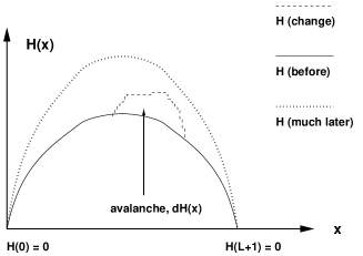
Figure 1: One-dimensional schematic example of the interface or history representation of a SOC model. The mean-field interface is parabolic, which implies that in the SOC steady-state $v(x)$ is parabolic, too. Notice the boundary conditions $H=0$ that ensure the loss of particles (equalling the increased elastic energy).

The SOC ensemble works (Figure (1)) so that the local force is increased in steps, by adding a grain at $x$ and making $F(x,t)\rightarrow F(x,t)+1$. Sometimes, $f>0$ and an avalanche starts. The interface moves at $x$ by one step, $\delta H(x)=1$. In the subsequent dynamics during the avalanche the columnar force term $F(x)$ does not change. The right choice of the interface boundary condition is $H=0$ which is to be imposed at two “extra sites” ($x=0$, $x=L+1$ for a system of size $L$ in $1d$). The $\langle F(t)\rangle$ increases slowly with time, so that the shape of the interface is on average a parabola. There are now three easy-to-define questions following from the SOC setup: i) can one understand the “avalanches” (bursts of activity) from the QEW depinning, with its presumably well-known exponents? ii) what is the effect of the parabolic interface shape on the physics of depinning, if any? (this relates to i) if things get complicated) and iii) how does the dynamics of such a driven parabola compare again to that of the “usual” QEW, if it is perturbed off the critical point?

The other model is simply constructed by considering activated random walkers. One puts $z_{x}$ of these per site, and the rules are such that if $z_{x}=1$ the walker is frozen, and for $z_{x}>1$ per unit time two walkers take off from $x$. This is in actual sandpile terms the Manna model [15], if the walkers are called “grains”. We have that $z_{c}=1$, and the toppling rule

$$z(x,t+1) = z(x,t)-2,$$ (11)

$$z(y^{\prime},t+1) = z(y^{\prime},t)+1,$$ (12)

$$z(y^{\prime\prime},t+1) = z(y^{\prime\prime},t)+1,$$ (13)

with $y^{\prime}$ and $y^{\prime\prime}$ two randomly chosen neighbor sites of $x$.

In the FES case (consider periodic boundary conditions) there is naturally a phase transition located at $n_{tot}\leq L$. Like in the QEW, the bare value of the control parameter (here $n_{tot}/L$) at the critical point is hard to compute. The important point is that the model is clearly an example of an “absorbing state” phase transition: any product measure of states with $z_{x}=1$ or 0 will do. Thus there is an infinite number of absorbing states, and moreover trivially $n_{tot}$ is conserved. These suffice to make it possible - and clear - that there can be differences to e.g. the contact process (this would amount in the random walker language to a model where walkers can die out, and have off-spring, moreover $z_{c}=0$), in the critical behavior.

In this model there is as well a memory effect: any configuration of grains in a local neighborhood is frozen till an avalanche sweeps over it readjusting the $z_{x}$’s. Note that the effect of this is diffusive since if a grain moves around, it does so by a simple diffusion process. The SOC ensemble is again obtained similarly to the LT automaton by allowing walkers to escape at the boundaries, and adding a walker at a time randomly ($z_{x}\rightarrow z_{x}+1$) if no active sites exist. In this case, it is easy (and easier than in the QEW case) see why there might be subtle differences between the two ensembles. The average $\langle z_{x}\rangle$ in the quiescent state between avalanches is created by the average flux of grains out of the system. In 1D, clearly any site for which $x\neq L/2$ there has to be a net flux of grains towards the absorbing boundaries. Thus the profile of $\langle z_{x}\rangle$ will for sure have a gradient as a function of $x$, giving rise to “finite size” effects that are difficult to analyze.

3 Sandpiles and absorbing states

The classical model for a system with an absorbing state is the “contact process”, where particles diffuse, die and are born as off-spring from neighboring ones on a lattice. In terms of a coarse-grained density-field $\rho$ one can illustrate its behavior with the mean-field equation

$$\frac{d\rho}{dt}=(\lambda-1)\rho-\lambda\rho^{2}$$ (14)

that includes the competition between the two mechanisms affecting the density $\rho$ [3, 61]. The MF-variant clearly has a phase transition at a $\lambda_{c}=1$, with $\rho=1-1/\lambda$ in the stationary state. The physics version on a lattice is directed percolation, which has as well an upper critical dimension $d_{u}=4$. The DP can be analyzed field-theoretically with standard coarse-graining techniques, and there is an extensive body of work on the critical exponents and scaling functions etc. for $d<d_{u}$.

The exponents that are of interest here are such that they describe the behaviorat the critical point and in its proximity. The former gives rise to $\nu_{\perp}$, $\nu_{\parallel}$, $z$, and $\beta$. These describe in turn the temporal and spatial correlation scales, the dynamics of the correlations, and the order parameter for $\lambda>\lambda_{c}$. One has the scaling relation

$$\bar{\rho}(\Delta,L)=L^{-\beta/\nu_{\perp}}R(L^{1/\nu_{\perp}}),$$ (15)

with $\Delta=\lambda-\lambda_{c}$ the distance to the critical point. $R$ is a scaling function with $R(x)\sim x^{\beta}$ for large $x$. For $L\gg\xi\sim\Delta^{-\nu_{\perp}}$ we expect $\bar{\rho}\sim\Delta^{\beta}$ using $\xi$ for the correlation length. When $\Delta=0$ we have that $\bar{\rho}(0,L)\sim L^{-\beta/\nu_{\perp}}$. Above the critical point the order parameter has a stationary value.

Such exponents and the scaling contained in Eq. (15) would then be the goal for an absorbing-state phase transition description of sandpiles. The example of activated random walkers aka the Manna model of the previous section makes it rather obvious that the FES ensemble - with the mild caveat that the transition should be continuous - might be described analogously to the DP. The Manna universality class is not expected to be in the DP universality class, due to the presence of the conservation law and the presence of an infinite number of absorbing states. The questions that remain are then highly non-trivial: first, what is the right effective field theory? Second, are there complications related to the specific character of the SOC ensemble?

The former of these two questions can be answered exactly for a class of stochastic models, with an infinite number of absorbing states, and with a static conserved field (NDCF, non-diffusive conserved field class). It is the coupling of this field to the order parameter evolution that creates a unique universality class [62, 63, 64]. This is a conjecture supported by extensive simulations of a number different models [62, 63]: a conserved threshold transfer process [65], a conserved lattice gas with repulsion of nearest neighbor particles, and a reaction-diffusion model (CRD) with two species of particles, $A$ and $B$. The exponents (in $2d$ ) are illustrated in Table I, together with the CP ones.

Steady state exponents $d=2$
	$\beta$	$\nu_{\perp}$	$\beta/\nu_{\perp}$	$z$	$\theta$
CTTP	0.64(1)	0.82(3)	0.78(3)	1.55(5)	0.43(1)
CRD	0.65(1)	0.83(3)	0.78(2)	1.55(5)	0.49(1)
Manna	0.64(1)	0.82(3)	0.78(2)	1.57(4)	0.42(1)
DP	0.583(4)	0.733(4)	0.80(1)	1.766(2)	0.451(1)

Table 1: Critical exponents for steady state simulations in $d=2$. Models: CTTP: Conserved threshold transfer process, CRD: Conserved reaction-diffusion model, Manna: Manna sandpile, DP: Directed percolation. From [64].

The conserved reaction-diffusion model studied in [63] has the pleasant feature that it can be mapped exactly, using a Fock-space representation and creation-annihilation operators [66, 67], into an effective action, or equivalently into a set of Langevin equations [63]. The resulting theory has, forgetting some naively irrelevant terms upon power-counting—, a structure proposed earlier on phenomenological grounds [68]. This set of equations reads

$$\frac{\partial\rho({\bf x},t)}{\partial t} = a\rho({\bf x})-b\rho({\bf x})^{2}+\nabla^{2}\rho({\bf x},t)-\mu\psi({\bf x},t)\rho({\bf x},t)$$

$$+ \sigma\sqrt{\rho(xv,t))}\eta({\bf x},t)$$

$$\frac{\partial\psi({\bf x},t)}{\partial t} = D\nabla^{2}\rho({\bf x},t)$$ (17)

For $\rho$, this looks like a Reggeon field theory [69] (used to describe DP) which is coupled to an extra conserved non-diffusive field, $\psi$. One thing is immediately clear, that is the theory contains a term that accounts for the memory of the dynamics of the grains in the model ($\phi$, again) which then couples to the actual activity $\rho$. These fields are also often called “energy” (grains) and “activity” (active sites), respectively. Due to the presence of this coupling the theory is non-Markovian.

Above, $\eta$ is a Gaussian white noise with a trivial correlator $\langle\eta({\bf x},t)\eta({\bf x}^{\prime},t^{\prime})\rangle\sim\delta({\bf x}-{\bf x}^{\prime})\delta(t-t^{\prime})$. The parameters ($a$ and so forth) are fixed. Notice the presence of the linear term, that orignates from the initial configuration. The effective noise strength is linear in the local density, since in the coarse-graining the activation and passivation of particles on the microscopic level becomes a Poissonian variable, with the variance equalling the expectation. In particular it vanishes for $\rho=0$.

The second equation describes how the conserved density diffuses upon the influence of actual activity. In the absence of such the dynamics is frozen. It can be integrated out formally, to obtain a single equation for the activity $\rho$. More concretely

$$\psi(x,t)=\psi(x,0)+D\int_{0}^{t}dt^{\prime}\nabla^{2}\rho({\bf x},t^{\prime}).$$ (18)

The first contribution in Eq. (18) follows from the initial condition, and is a “quenched” term: it is frozen and not affected by the presence of the thermal noise. The second is a non-Markovian term. The theory as it stands has one easy consequence: $d_{u}=4$ (though there is a claim by Wijland that in fact $d_{u}=6$ [70]) in agreement with numerics on this universality class. The problem is that Equation (3) is difficult to renormalize due to the presence of the extra terms (in addition to the DP-RFT) [64]. Thus one has no useful predictions as such. In the next section we discuss the relation of SOC to depinning, in which case the corresponding situation in the QEW becomes pertinent. For quenched depinning the lesson is that the quenched noise field renormalizes in a highly non-trivial fashion (in particular from the viewpoint of the technicalities of the computations). Here an analogy would be the correlated activity that reflects the landscape (grains or particles), at various instances of time.

It should also be noted that the theory of Eq. (3) fails in the presence of a number of effects - or does not hold of course for all possible sandpile models. The BTW model has no randomness in the toppling rules, its conservation laws play a role and the situation is different [21]. For the LIM automaton of the previous section, the additional quenched noise clearly plays a role in the way the activity stops (or is “pinned”). The question what the NDCF class means as a depinning problem will be discussed in the next section, but it is worth underlining that the connection between the two kinds of transitions would merit further study [71].

The SOC state in the FES case arises on a simplistic level by combining an absorbing state with another demon (a close cousin of the BTW one), with the task of driving the system if $\rho=0$, everywhere. This is combined by a dissipation (like the boundary losses) that ensures that for $\rho>0$ $d\rho/dt<0$. This is of course just a complicated way of stating the simple rules of CA’s (since we know that the state is such that $\langle\rho\rangle=0^{+}$ due to the separation of timescales with respect to dissipation and driving). Technically this implies that $\langle z_{x}\rangle$ in the SOC case is limited above by the critical value of the FES critical point. This is trivially so since the opposite would imply that $\langle\rho_{x}\rangle>0$, locally for some $x$. The actual scaling function of $\langle z_{x}\rangle({\bf x},L)$ is however not known. This is in fact one of the fundamental questions of SOC sandpiles: if one can separate “bulk” behavior from boundary effects.

Recent work by Dickman has shown that precisely at the SOC critical point the sandpile avalanche properties obtain logarithmic corrections to their scaling functions with $L$. This surprising finding implies that the finite size scaling in the SOC ensemble is not easy to understand based on the translationally invariant FES (or depinning case). This would also be expected to hold in general for the NDCF-class (for all its models in the SOC ensemble).

Notice however again that the description in terms of the coarse-grained theory invites for two other scenarios: clearly the critical point can be approached by any suitable dissipation mechanism, not only the boundary loss -one. A possibility is bulk dissipation (e.g. a constant probability per step that a diffusing grain is removed). Such perturbations are closer to the FES case, since translational invariance is restored.

4 SOC models and depinning

4.1 Interfaces in random media

Rough interfaces [72, 10, 73, 74] are objects with “self-affine” geometry. They can move due to an applied force, such as a magnetic field or a pressure difference. The essential point is that the thermal fluctuations may be neglected, if the noise is due to the presence of impurities or defects in the material. Such disorder is quenched, static in time. The interface can get locally pinned, if a local “pin” is strong enough to overcome (generalize) surface tension. A characteristic example is the quenched Edwards-Wilkinson (QEW), or linear interface model (LIM) [59, 60, 58]:

$$\frac{\partial H}{\partial t}=\nabla^{2}H+\eta(x,H)+F.$$ (19)

Here $H$ is driven by $F$, and the combination of the surface tension and the randomness $\eta$ gives rise to the critical behavior. In particular, depinning takes place at a force $F$ close to a critical value $F_{c}$. Depinned interfaces move with a velocity (order parameter) $v\sim f^{\theta}$, with $f=F-F_{c}\geq 0$. Pinned interfaces are blocked by “pinning paths/manifolds” which arise from the quenched disorder in the environment.

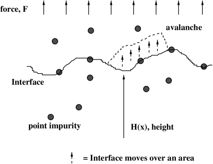
Figure 2: An interface in a random enviroment: a part moves under the influence of $F$, the rest is pinned.

The description of kinetic roughening involves analogously to the absorbing state phase transitions a correlation length $\xi$. Statistical scale invariance assumes (statistical) translational invariance, developing both in time and space [72, 10]. The typical quantity to measure is the roughness (mean square fluctuation) $w_{q}(L,t)$, where $L$ is the measurement scale. One often observes power law scaling for its moments,

$$w_{q}(L,t)\equiv\langle\langle\delta H({\bf x})^{q}\rangle\rangle^{1/q}\sim L^{\chi_{q}}\mbox{ for }L<\xi(t)$$ (20)

saturating to a constant for $L$ larger than $\xi$ (the inner brackets imply averaging over ${\bf x}$, and the outer an ensemble average). $\chi_{q}$ is called $q$-th order roughness exponent, allowing for multiscaling should the $\chi_{q}$ differ from each other (as for “turbulent interfaces”[75], when the correlations are dominated by the largest height difference between two neighboring points, $\Delta H=|H_{x+1}-H_{x}|$ [75, 76, 77]).

Usual self-affine scaling means $\chi_{q}\equiv\chi=\mbox{const}$, and $\xi(t)$ increases as $\xi(t)\sim t^{1/z}$, with $z$ the dynamical exponent. The maximal extent of interface fluctuations

$$w(t)\equiv\lim_{L\to\infty}w(L,t)\sim\xi(t)^{\chi}\sim t^{\chi/z}\equiv t^{\beta},$$ (21)

which defines the exponent $\beta$, combining into a scaling form

$$w(L,t)=\alpha(t)\;\xi(t)^{\chi}\;\mathcal{W}\left(\frac{L}{\xi(t)}\right).$$ (22)

with the scaling function $\sim x^{\chi}$ for $x<1$ and a constant for $x\gg 1$. If the amplitude $\alpha(t)$ increases, so-called anomalous scaling ensues [78], and if $\chi>1$ ”superroughness” [78, 79]. The LIM in $1d$ is an example [58, 80, 81, 82], and below we will discover that several SOC automata in the interface description have this property as well. $\chi$ can also be described by the structure factor, or spatial power spectrum

$$S({\bf k},t)\equiv\langle|h({\bf k},t)|^{2}\rangle\sim\Biggl{\{}\begin{array}[]{ll}\!k^{-(2\chi+d)}&\mbox{for }k\gg 1/\xi(t)\\ \!\xi(t)^{2\chi+d}&\mbox{for }k\leq 1/\xi(t)\end{array}$$ (23)

where $h({\bf k},t)$ denotes the spatial ($d$-dimensional) Fourier transform of $h({\bf x},t)$. Also, the height difference correlation function $G_{2}({\bf x},t)\equiv\langle|h({\bf x},t)-h(0,t)|^{2}\rangle^{1/2}=\int_{\bf k}S({\bf k},t)\left(1-\cos({\bf k\cdot x})\right)$ can be used, but note that it reflects only the local roughness exponent $\chi_{\rm loc}$ and thus for superrough interface, with $\chi>1$, one needs $S$ (for $L$ fixed). For temporal quantities the analogue is naturally the power spectrum, in the stationary state, $S({\bf x},\omega)\equiv\langle|h({\bf x},\omega)|^{2}\rangle$ (which has obvious problems in the SOC state, due to the separation of timescales), or correlation function of the $q$th moment of height “jumps” over a temporal distance $t$

$$C_{q}({\bf x},t)\equiv\langle|h({\bf x},t+s)-h({\bf x},s)|^{q}\rangle^{1/q}.$$ (24)

Generally one finds an increase $C_{q}({\bf x},t)\sim t^{\beta_{q}}$ over “short” time distances $t$. In the case of (conventional) scaling it is related to the early time increase of the width, $q$-moments $\beta_{q}\equiv\beta=\chi/z$. It is easier to use than $w(t)$ at early times.

The main universality class of the QEW, Eq. (19), is reached for random bond and random field disorder (these flow in the RG into the same fixed point). The RF noise correlator reads

$$\langle\eta(x,h(x,t))\eta(x^{\prime},h(x^{\prime},t^{\prime}))\rangle=\Delta(h(x,t)-h(x^{\prime},t^{\prime}))\delta(x-x^{\prime})$$ (25)

where $\Delta(u)$ is in practice taken as a delta function, $\Delta(h(x,t)-h(x^{\prime},t^{\prime}))\rightarrow\delta(h(x,t)-h(x^{\prime},t^{\prime}))$. If the velocity $v$ is finite, the average motion and the fluctuations separates, hence for $l_{th}>(vt)^{1/\chi}$,

$$\delta(h(x,t)-h(x^{\prime},t^{\prime}))\rightarrow\delta(v(t-t^{\prime})+\delta h)\rightarrow\frac{1}{v}\delta(t-t^{\prime})$$ (26)

the noise becomes thermal, with the strength $\tilde{\Delta}=\Delta_{0}/v$, and $\langle\eta(x,t))\;\eta(x^{\prime},t^{\prime})\rangle=2T\delta(x\!-\!x^{\prime})\delta(t\!-\!t^{\prime})$. The QEW becomes then the normal Edwards and Wilkinson one, for a surface relaxing by surface tension [10].

The QEW develops critical correlations in the vicinity of the critical point, $F_{c}$. The standard analysis of the problem is the functional renormalization group method. One-loop expressions for the exponents are found in papers by Nattermann et al. and Narayan and Fisher [60, 59]. The analysis has been pushed recently further by Le Doussal, Wiese and collaborators [83] illuminating several open issues. The main fixed point is the RF one, but for correlated noise there is the possibility of continuously varying exponents. The upper critical dimension is $d_{c}=4$, above which mean-field theory applies. Several exponent relations exist close to the critical point, like $\theta=\nu(z-\chi)$ for the velocity exponent, and $\chi+1/\nu=2$. This, together with the $\theta$-exponent relation, tells that there is only one temporal and one spatial scale at the critical point.

For the RF fixed point, the 1-loop functional RG results are $\chi=(4-d)/3$, and $z=2-(4-d)/9$. Later work by Chauve, Le Doussal, and Wiese [83] yields (with $\epsilon\equiv 4-d$) $\zeta=\frac{\epsilon}{3}(1+0.14331\epsilon+\dots)$. In particular in $d=1$, this means that the RG beyond one loop is better able to adhere to the numerical LIM results [58, 60, 84] with a superrough interface ($\chi_{{\rm QEW},d=1}\sim 1.2\dots 1.25$). Note that the depinning problem can also be discussed in the constant velocity ensemble, which allows for the presence of avalanches (since parts of the interface are pinned close to $F_{c}$) in the presence of translational invariance [85, 86].

There is one “easy” case in which one can understand SOC with depinning, “at once”. This comes in the form of the $1d$ Oslo ricepile model [87], which operates on the idea of having slopes $z_{i}=n_{i}-n_{i+1}$, at each site, which are compared with a critical slope $z_{c}$, either one or two. The dynamics is such that a overcritical site gives one grain to its right neighbor, and thus decreases $z_{i}$ by $2$, while its nearest neighbors’ increase one. After each toppling $z_{c}$ is redrawn from a probability distribution. If there are no active sites, the avalanche stops and the model is driven at the boundary ($i=1$). Paczuski and Boettcher noticed that this can be mapped, (since $z_{i}$ changes as an elastic force term) into a boundary-driven LIM [5], and conjectured that the discrete equation is in the LIM class. Recently Pruessner has shown that one can do the mapping in a slightly different way, which allows to get around the delta-functions involved in this particular model systematically [88].

4.2 Mapping SOC to interfaces: the noise

One would like to describe sandpiles with the dynamics of the “interface”, of the history of the sandpile, as in the discrete version of a QEW of Section II, the Leschhorn automaton. For this purpose it is also instructive consider some other models than the “LIM” sandpile, the BTW and the Manna ones [8].

The Zhang model [16] resembles both the BTW model and the Manna model in that the topping rule is a combination of deterministic and stochastic factors. It is defined in with a continuum ’energy’ $z$, with the dynamics

$$z(x,t+1) = 0,$$ (27)

$$z(y,t+1) = z(y,t)+z(x,t)/2d,$$ (28)

and $z_{c}=2d-1$. These imply that the ’energy’ of a critical site is divided equally between the neighbors. The drive in the Zhang model is usually, in the SOC case, implemented so that the energy is increased by small, finite amounts at a random site $x$. Or, one picks the site closest to $z_{c}$, since it will typically sooner or later be the one to reach criticality first. In the Zhang model the detailed history of topplings is of importance making serial and parallel dynamics for active sites to differ. Note that the Leschhorn (QEW) automaton and the BTW one are Abelian (as is the Manna model, in the general sense), so that it explicitely does not matter if parallel or serial topplings are used.

Another widely studied model is the Olami-Feder-Cristiansen (OFC) model [89], usually studied in the following deterministic version. The system is prepared with an initial (continuum) energy profile $z(x,0)$ and a threshold $z_{c}$ is chosen. Now, define a distribution parameter $\alpha$. With the aid of $\alpha$ the OFC model reads if $z_{x}>z_{c}$

$$z(x,t+1) = z(x,t)-z_{c},$$ (29)

$$z(y,t+1) = z(y,t)+\alpha z_{c},$$ (30)

with $\alpha\leq 1/4$ in $2d$ . The point of dissipation ($\alpha<1/4$) is that one can achieve a steady-state even if the open boundary conditions are replaced with e.g. periodic ones. The same trick can also be applied to any of the previous models, where one can do away with dissipative boundaries, and substitute for that with a small but finite removal rate of grains that topple [14].

A third case, very similar to the Manna, is a microscopic model in the NDCF class [63]. Consider a two-species reaction-diffusion process, with particles of types $A$ and $B$ involved. At each site $i$, and at each (discrete) time step the following reactions take place:

$$B_{i} \rightarrow B_{nn}\,,\,\,r_{d}(\equiv 1)$$ (31)

$$A_{i}+B_{i} \rightarrow 2\times B_{i}\,,\,\,r_{1}$$ (32)

$$B_{i} \rightarrow A_{i}\,,\,\,r_{2}.$$ (33)

The $A_{i}$, $B_{i}$ denote particles of each kind at site $i$. $r$’s are the probabilities for the microscopic processes to occur: diffusion, $r_{d}$, activation $r_{1}$, and passivation $r_{2}$. Fix $r_{d}=1$, implying that, after having the chance to react, $B$ particles diffuse with probability one, and a phase boundary follows between the active and absorbing phases in terms of the $r_{1}$, $r_{2}$ probabilities. For occupation numbers $n_{A,i}$, $n_{B,i}$ per site, since the $A$’s are non-diffusive, there is an infinite amount of absorbing states defined by $n_{B,i}=0$ for all $i$, with $n_{A,i}$ arbitrary, similarly to the Manna model [71].

The idea of how to map the dynamics of sand in these models into a noise term is similar to the microscopic arrival-time mapping which connects directed polymers in a random medium to the temporal behavior of a roughening interface, governed by the Kardar-Parisi-Zhang equation [10]. It is also a cousin of ’run-time statistics’ by Marsili et al., which maps the quenched disorder in say invasion percolation to an effective memory term at each location [90]. The ensuing noise in a sandpile LIM arises from annealed to quenched disorder mappings.

Essentially, one constructs the “local force” ($f$) by looking at how $z_{x}$ deviates from its expected value at the time of toppling. This is obtained by considering the net effect of the sandpile rules, by decomposing via a projection trick the expected incoming grain or energy flux as

$$n_{x}^{in}=\bar{n}_{x}^{in}+\delta n_{x}^{in},$$ (34)

where $\bar{n}_{x}^{in}$ measures the expected flux into site $x$ up to time $t$ and $\delta n_{x}^{in}$ is the deviation. The average part can be used to construct a Laplacian, while $\delta n_{x}^{in}$ generates a noise term

$$\tau(x,H) = \delta n_{x}^{in}\equiv n_{x}^{in}-\bar{n}_{x}^{in}$$ (35)

$$= n_{x}^{in}-\nu\sum_{x_{nn}}H(x_{nn},t).$$

The sum over the nn’s in Eq. (35) is the average grain flux into $x$ due to each toppling of a nn, computed exactly at the time of toppling at $x$ at height $H$. For the reaction-diffusion model one needs to define $H$ by the integrated activity of $B$-particles, so that one $B$ diffusing out of $x$ means a “toppling”. Then the flux fluctuates since $B$’s diffuse, randomly, while the reactions between the $A$ and $B$ species are accounted for every time $B$ particles leave the site ${\bf x}$. Ie., one considers $n_{A}$ and $n_{B}$ when the site becomes active and a particle diffuses out. Then $n_{tot}(x,H)=n_{A}({\bf x},H)+n_{B}({\bf x},H)$.

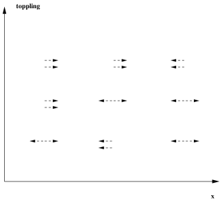
Figure 3: How the randomness maps to an interface noise field in the Manna model in 1d: each toppling implies one expected grain at a nn, but can give zero or two instead (contributing to $\delta n_{nn}^{in}$).

In the case of the Manna model, each nn-toppling contributes $1/d$ to $\bar{n}_{x}^{in}$ and thus $\nu=1/d$ while for the others the average flux is dependent on the average energy at the time of toppling,

$$\delta n_{x}^{in}=n_{x}^{in}-z_{av,c}\sum_{nn}H_{nn}.$$ (36)

Here $z_{av,c}$ is the above average energy in the Zhang and OFC models, contrary to the Manna model this is not known a priori. Another way to write the fluctuation term is $\delta n_{x}^{in}=\sum_{H_{nn}}\delta z_{H_{nn}}$, ie. the fluctuations consist of sum of the differences between the real amount of energy of the toppling neighbors and the expected average energy. This makes it evident that though the Zhang and OFC model will have the same columnar noise from the drive as the others, another component is born out of the the sandpile rules.

In the RD-model, the noise takes into account that since after a toppling a passive site can get activated only after a nn topples, and since the reactions make $n_{B}$ fluctuate while it is non-zero. Thus if and only if a site does not topple during a time step, it implies that there is an effective threshold so that $n_{B}-n_{c}<0$ or that $n_{B}=0$. These give rise to a $\tau$-distribution, that depends upon the total number of particles after the preceding toppling and the microscopic dynamical rules at a site. The immobile grains $n_{A}$ imply a “pinning force”, as a large $n_{A}$ for a constant $n_{tot}$ reduces the probability to topple.

The noise $\tau(x,H)$ is dependent on the choice of dynamics or the toppling order, and this becomes important if the model is not Abelian (the Zhang model) Keep in mind, that the mapping describes any particular sandpile with an interface, which follows exactly the same dynamics. For any change of dynamics this implies that the noise field has to change as well. The $f$ of the discrete interface equation reads thus

$$f=\nu\,\,\nabla^{2}H+F(x,t)-z_{c}(x,H)+\tau(x,H)$$ (37)

allowing for varying $z_{c}$ for the sake of generality, with $\nu=1/d$ for the Manna.

The other source of “SOC” noise arises since the implied step-function, $\theta(f)$, in Equation (8) forces the corresponding interface to move only forward, so that the velocity $v\equiv\Delta H/\Delta t$ is either 0 or 1 [58]. This can also considered as an origin of noise, a term $\sigma(x,H)$. An illustration is shown in Fig. 4. On the avalanche timescale $f<0$ at site $x$ and $f$ increases until at time $t-1$ one or more neighbors topple resulting in $f>0$. Then site $x$ topples at time $t$. Thus the sandpile rules result in an effective force $f^{\prime}\equiv 1$, acting on $H$ as $\Delta H/\Delta t=f^{\prime}\,\theta(f)\equiv f^{\prime}\theta(f^{\prime})$. The relation between $f$ and $f^{\prime}$, valid for as long as $H$ is constant, is

$$f^{\prime}(x,H)=f(x,H)+\sigma(x,H),\,\,\,\,\,\,\,\,\,\sigma(x,H)=1+z_{c}(x,H)-z(x,t^{*})$$ (38)

where $t^{*}$ is the time at which site $x$ topples. This means specifically that one can construct $\sigma(x,H)$ as a quenched random variable, at $t^{*}$, as if it were noise included in a QEW from the very start. It is computed from the difference between $f$ and $f^{\prime}$ when $x$ topples. $f^{\prime}$ and $f$ are time-dependent, they change as grains are moved, or the Laplacian changes. The equation $\Delta H/\Delta t=f^{\prime}\theta(f^{\prime})$ can finally be viewed as the discretization of the continuum equation $\partial H/\partial t=f^{\prime}$.

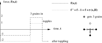
Figure 4: Rescaling of the force $f$ and an example of how the $\sigma$-noise ensues (three grains added simultaneously) due to “extra” grains present when the site topples.

4.3 Sandpiles at criticality

Such mappings result in the discretized interface equation

$$\frac{\partial H}{\partial t} = \left(\nu\nabla^{2}H+\eta(x,H)+F(x,t)+\sigma(x,H)\right)$$ (39)

$$~{}~{}~{}\times\theta\left(\nu\nabla^{2}H+\eta(x,H)+F(x,t)+\sigma(x,H)\right),$$

with the surface tension $\nu$ depending on the model, and with $\eta(x,H)=-z_{c}(x,H)+\tau(x,H)$. This is the central difference discretization of the LIM, and parallel dynamics are usually assumed. The physics of such an equations contains the Laplacian character of grain dynamics, which corresponds to the elasticity. topplings map exactly to an elastic force. The sandpile dynamics (a toppling) is translated into a force $\eta+F$, that manages to overcome a pinning force, so that the interface moves by one step. The rules of the individual sandpiles are embedded in the noise variables [$F$, $\eta(x,H)$] as do the details of the dynamics [$\sigma$]. The ensemble (SOC, FES or depinning etc.) is reflected in the boundary conditions, eg. $H=0$ at the boundaries. The character of the criticality is therefore determined by a combination of these two: noise, and ensemble.

The theoretical understanding of the relevance of the noise terms implies that pertubations of the type $\eta$ are relevant, and lead to the establishment of unversality classes that depend on the RG flow of the noise field upon rescaling. In particular, there is the LIM/QEW class. As discussed earlier the NDCF/Manna class defines another one, characterized by a different set of exponents. The upper critical dimension of the LIM is $d_{u}=4$ for all cases, however, because of the Laplacian in Eq. (39). Table 2 lists some recent numerical results of Chate and Kockelkoren [91]. The BTW model presents a different story, due to the fact that the continuum and discrete versions differ (as we discuss below in the context of the $\sigma$-term). Notice that its continuum version is directly solvable, and corresponds to the deterministic relaxation of an initial height profile in the absence of noise, of any type. This is since the height profile can be recast into a form that accounts for $F(x,0)$. For the OFC and Zhang models the situation is not so clear - they both present deterministic dynamics during the avalanches, ie. an absence of explicit noise terms of the type $z_{c}$, but $F(x,t)$ is still present.

While $\eta(x,H)$ term in the LIM case has an exact equivalence $z_{c}(x,H)=\eta(x,H)$, implying point disorder, the noise field for the NDCF class, including the Manna model has a noise field $\tau(x,H)$ which is point-like but correlated. This is since $\tau$ is conserved,

$$\sum_{x,H(x)}\tau(x,H)\equiv 0$$ (40)

in the case of a closed system (periodic boundary conditions, e.g. the fixed energy ensemble), and approximately for the SOC one. The average of $\tau$ is zero, $\langle\tau\rangle=0$. For the Manna model at any particular $x$ the increments of $\tau$ are random walk -like, since the neigboring sites’ topplings constitute a random point process. Define the noise two-point correlation function by

$$C(\Delta x,\Delta H)=\left<\tau(x+\Delta x,H+\delta H)\tau(x,H)\right>,$$ (41)

where an average is performed over the ’disorder’, or in the sandpile sense many toppling histories. The random walk-character of the $\tau$ means that

$$C(\Delta x,\Delta H)\sim f(\Delta x)(\Delta H)^{1/2}$$ (42)

since the increments are uncorrelated at a singel $x$, and $f$ denotes a correlator in the $x$-direction. This kind of noise correlations are similar to the ABBM-model of Barkhausen noise. The character of the $x$-part of the noise correlator for the Manna-model is more subtle (note that one might also study such a LIM, but with $\tau(x,H)$ changing after each toppling with uncorrelated increments). In the SOC ensemble the interface will be parabolic, in such a way that at a constant $H$ the various noise values $\tau(x,H)$ decorrelate so that one should perhaps measure the noise correlator along the interface. Since it is the sandpile dynamics that gives rise to $\tau$, its local value should be related in a non-trivial way to the local interface height. Even more simply, if a site gets by chance very few grains compared to the expectation, then it does not topple very much ($H<\bar{H}$) and $\tau(x,H)$ is negative. In the FES case $f$ can be defined and measured e.g. numerically in the standard fashion, but $C\sim f$ should decay quickly since neighbors have a weak influence on each others’ noise values $\tau$ (see Fig. 3). They correlate in the noise strength since the $H$-part of the correlator is dependent on the interface height. The case of the RD model is slightly more complicated, though the noise from the diffusive flux is the same as for the Manna, explaining qualitatively the existence of such a NDCF universality class. The off-critical behavior of such models couples directly the noise field, unlike in a LIM-automaton, and might have to do with the observation of slow relaxation in the Manna model [92].

Keep in mind that what matters in determining avalanche properties is the effective disorder that influences its spreading. In the models with $\tau$-noise this means that increments of $\tau$ stem from randomness in the rules (and the noise correlator $C$ above measures its feedback on the avalanche dynamics). For other models (BTW, Zhang, OFC without additional disorder) the avalanche dynamics does not experience any randomness “during” the avalanche, but are set by the initial properties of the system. Eg. though for Manna $\tau$ is conserved, in the case of the Zhang model (say) the average $\tau$ during an avalanche can be different from zero, though its ensemble average is zero. It is also possible to drive a SOC-interface with strong enough randomness so that the interface tension vanishes. In sandpile language this can be achieved by making e.g. the toppling thresholds increase (even without bounds). Then a natural possibility is a cross-over to directed percolation, precisely since the diffusive grain dynamics is changed, by the extra noise [93].

The fixed energy ensemble [13, 68] corresponds to ordinary depinning, ie. $H(x,t=0)=0$, $F(x,t)=F(x,0)$, and periodic BCs, with no dissipation. One needs to tune the control parameter $\Delta F=n_{tot}/L^{d}$, to obtain criticality, to $\Delta=0$. The usual “random preparation” of the grain configuration corresponds to a spatially dependent force profile $F(x,0)$, which might give rise to some memory effects, depending on its exact (columnar) form [94]. In the same vein, “microcanonical” simulations [95] one has dissipation operating on the slow time scale with exactly the same rate as $F(x,t)$. Thus microcanonical simulations correspond to fixed energy simulations with a specific initial configuration: after each avalanche, the time is reset to zero, the force is replaced with $F\to F+\nabla^{2}H$, and the forces at $x^{\prime}$ ($x^{\prime\prime}$) are increased (decreased) by one unit where $x^{\prime}$ and $x^{\prime\prime}$ are randomly chosen sites. Finally the interface is initialized, $H\equiv 0$. Recent simulations of the NDCF/Manna (or Conserved-Directed Percolation, C-DP) class in the depinning ensemble have revealed, that the scaling exponents are in $2d$ very close to LIM, while in $1d$ and $3d$ differences ensue [91, 96, 65]. In particular, there is the $\kappa$-exponent that relates the local and global roughness exponents ($\chi_{global}=2\kappa+\chi_{loc}$,, as a clear signal of anomalous scaling (and in $1d$ of superrough behvior) [91, 96]; the . The BTW model is in a different class as such, due to the extra symmetries, and as expected based on the presence of noise in the other models [97].

Table 2: Critical exponents of the C-DP/NDCF class in $1d$, $2d$, and $3d$. The corresponding values for DP and LIM are also given for reference. From [91].

$d$		$\delta$	$z$	$\beta$	$2\kappa$
	DP	0.1596	1.58	0.2765	0.84(1)
1	C-DP	0.140(5)	1.55(3)	0.29(2)	0.86(1)
	LIM	0.125(5)	1.43(1)	0.25(2)	0.35(1)
	DP	0.451	1.76	0.584	0.56(2)
2	C-DP	0.51(1)	1.55(3)	0.64(2)	0.50(2)
	LIM	0.50(1)	1.55(2)	0.63(2)	$0^{+}$
	DP	0.73	1.90	0.81	0.30(5)
3	C-DP	0.88(2)	1.73(5)	0.88(2)	$<0.2$
	LIM	0.77(2)	1.78(7)	0.85(2)	0

For open boundary sandpiles, the right interface boundary condition is $H=0$ which is to be imposed at “extra sites” ($x=0$, $x=L+1$ for a system of size $L$ in $1d$). In the SOC steady-state the Laplacian increases, because of the parabolic shape for the the toppling profile $H(x)$ (see also [98]; $\rho$ in the APT-picture naturally equals the same). This is compensated by the ever-increasing $\langle F(t)\rangle$, or the addition of grains by the SOC drive. Writing now $\langle F\rangle\equiv ft$, and $H\equiv H_{x}t$, one has the Poisson equation

$$\nu\nabla^{2}H_{x}=-f_{x}$$ (43)

with the constraint that $H=0,x\in\partial x$, and the source term $f_{x}=0,\partial x$ and $f_{x}=f$, elsewhere. This formulation of the ’history’ of topplings in a sandpile is just another way of looking at the lattice Green’s function for any sandpile, noticed by Dhar in the case of the BTW long ago [99].

Concerning the fluctuations, at the depinning critical point an interface has a diverging response. In the sandpile language the average avalanche size diverges with system size,

$$\left<s\right>\sim L^{2}$$ (44)

which follows also from the fact that each added grain will perform (an effective random walk) of the order of $L^{2}$ topplings before leaving the system, independent of dimension [13, 100]. In Eq. (43) the rate of divergence is reflected in $\nu$, in that it measures for each particular choice of rules how the above scaling can be interpreted as an equality, since the total number of topplings per grain added is dependent on $\nu$. The linear relation between $\nu$ and the interface velocity does in no way reflect the actual universality classes of the models. It just manifests the fact that the critical point of such models exhibits “anomalous diffusion”, as hinted by the LIM dynamical exponent $z\neq 2$. Hence in the interface representation such glassy response is easy to understand [101].

Recall that in the SOC steady-state the probability to have avalanches of lifetime $t$ may have the distribution $P(t)=t^{-\tau_{t}}f_{t}(t/L^{z}).$ $P(s)$ was mentioned in the Introduction, and $s\sim t^{D_{s}/z}$ and $z(\tau_{t}-1)=D_{s}(\tau_{s}-1)$. The linear size $\ell$ related to $s$ scales as $s\sim\ell^{D}$ and the (spatial) area as $\ell^{d}$ (for compact avalanches) with $\ell$ the linear dimension. Thus, $\tau=2-2/D$ and $\tau_{t}=1+(D-2)/z$. From the interface depinning picture we now obtain directly that the “volume” of an avalanche should scale as $d+\chi$, and that the average area scales as $\left<\ell^{d}\right>\sim L^{1/\nu}$. The former implies the important scaling relation

$$\tau_{s}=2-2/D=2-2/(d+\chi).$$ (45)

This holds if and only if simple self-affine geometry can be expected. The avalanche exponents of SOC models are notoriously hard to measure, making it for a long time apparent that e.g. the BTW and Manna models would be in $2d$ the same universality class, with $\tau_{s}\sim 1.27$ for instance [102, 103, 104]. In the light of connection to interface depinning and (Manna, only) to NDCF class this seems fortuitious at once. The constant-velocity ensemble is a “good” one for checking out Eq. (45), and indeed for the LIM class the expected avalanche scaling can be found [86]).

For the SOC case, recent simulations have unearthed two fundamental facts. First, the dissipating avalanches can have interesting properties of their own [105]. In the BTW model this is related to the fact that the avalanche stops at once when the boundary is met, while for the other models this holds as a strong trend [22]. More importantly, the existence of multifractal behavior has been demonstrated, also in the BTW, by Stella and coworkers [24]. This presumably follows from the strong symmetries present in it; one can also measure many interesting quantities in the “wave picture” [21, 106, 107]. of the BTW, which are naturally hard to relate to any scaling theory related to interfaces or absorbing states. In concrete terms, the multiscaling indicates that for e.g. the avalanche sizes various momenta exhibit different scaling exponents $\tau_{s,q}$, as a function of the pile size $L$, $\langle s^{q}\rangle\sim L^{\tau}_{s,q}$. For the Zhang model, Pastor-Satorras and Vespignani have used the same technique to point out the lack of any clear scaling whatsoever. This model can combined with randomness, in which case the scaling attained is that of the NDCF/Manna-class. Likewise it seems possible to pertub a SOC state continously (in terms of the effective scaling exponents) between the Manna and the Zhang model endpoints [108]. This seems to follow naturally in the light of change in the effective noise acting on the interface representing the sandpile. In the same vein, the existence of strong, Manna-type noise is a relevant perturbation and explains the cross-over to similar scaling exponents, if such randomness is added on the top of the other sandpile rules [109].

Recent work by Dickman has shown however that more fundamental surprises can be found in the NDCF avalanche properties [110]. Fig. (5) depicts the result of careful numerical simulations, demonstrating that one needs systematic logarithmic corrections to describe the $P(s)$-distribution [111]. That is,

$$P(s)=s^{-\tau_{s}}(\ln s)^{\gamma}f_{s}(s/s_{c}),$$ (46)

where $\tau=1.386$ $\gamma=0.683$, for the Manna model in $2d$ ($1d$ data did not show evidence of such corrections). $f^{*}$ (see the caption) fluctuates about a constant over the optimum fitting interval, while the effective $\tau$ varies strongly in the same. The figure also has a pure power-law fit, with the estimate $\tau_{s}=1.25$ [103]. The latter yields a strongly curved function $f^{*}(x)$, and shows that a power-law is not a good description.

Figure 5: Plot of $f^{*}=s^{\tau}P_{s}(s)/(\ln s)^{\gamma}$ versus $\ln s$ for the data shown in Fig. 1. Lower curve: best-fit for $3<\ln s<10$ using $\tau=1.385$ and $\gamma=0.672$; upper curve: pure power-law fit using $\tau=1.25$. From [111].

The next candidate, to establish the validity of Eq. (45), is then the LIM model. It also allows to use the geometry of the “pinning paths”, if the SOC and normal critical states are directly connected. In directed percolation depinning (DPD), the geometry of the random quenched landscape leads to a self-affine picture of the interface dynamics, described by the quenched KPZ equation [72, 10]. The interface motion takes place so that the interface invades the voids (constituting avalanches) of multiconnected network of pinning paths, and thus the sizes of the avalanches are related to the void sizes. This is given by (in the LIM case) the structure of an “elastic percolation problem” [112], so that the the RHS of the qEW is always negative semi-definite, $f\leq 0$. There are two fundamental issues: how the scaling of voids, the relation of size vs. area is described with an appropriate roughness exponent, $\chi_{loc}$, and what is the probability to produce an avalanche if the interface is unpinned at a particular spot ([113, 114, 115]). In analogy with DPD [113], it follows that

$$\tau_{s,dep}=1+(1/(1+\chi_{loc}))(1-1/\nu)$$ (47)

which using the global $\chi\sim 1.20\dots 1.25$, produces

$$\tau_{s,dep}\approx 1.08.$$ (48)

This is the same as the prediction of Eq. (45), showing that assuming strict self-affine avalanche scaling the SOC and depinning ensemble predictions for $\tau_{s}$ (and other such exponents) coincide.

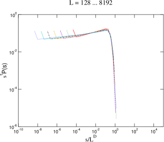
Figure 6: A data collapse using $\tau_{s}\sim 1.08$ and $D_{s}\sim 2.20$ for the LIM-SOC model (Leschhorn-type automaton, unpublished).

Figure 6 shows a representative scaling plot of SOC simulations of a $1d$ qEW/LIM, of the Leschhorn-type. System sizes upto $L=8192$ have been studied, with 2 $\times$ 10⁶ avalanches for the largest $L$. It is rather evident that the bulk part of the distribution does not collapse that well, for the largest system size the fitted effective $\tau$ is way off from the predicted 1.08 (1.024 for $L=8192$). An attempt to fit the exponents to an asymptotic value and a correction implies $\tau_{s,SOC}(\infty)\sim 1.115$, clearly off the expected value.

Thus, in analogy to the $2d$ Manna model, it seems that the ensemble here is of importance, or in the interface language the parabolic interface profile. It would be of interest to attempt such comparisons in higher dimensions, where one needs more exponents (or assumptions to describe the probability distributions since the avalanches have in addition to an area vs. volume relation also a perimeter length vs. area relation [116, 114]). One would expect in any case that $D_{s}\leq d+\chi$ for the cut-off dimension, since the SOC state can of course not be ’over-critical’.

Surprises in trying to match the translation-invariant non-equilibrium phase transition and the SOC one present the question whether the differences vanish asymptotically, so that the exponents of the statistically homogeneous ensemble are recovered? The other possibility is that the SOC ensemble is an independent one. Microscopically, this would result from a non-uniform density of grains (or average force acting on the interface). In $1d$, a site $x$ will get a larger grain flux from its neighbor on the bulk side and a smaller one from the boundary side - more trivially, there is a net flux of grains towards the boundaries.

This can be stated a bit less casually by considering the integral of the deviation from the force at depinning criticality, at $x$, $\Delta F(x)=F_{dep}-F(x)_{SOC}$, where $F_{dep}$ and $F(x)_{SOC}$ are averages at the critical points of the ensembles. This implies e.g. a finite-size correction to the normal critical point, $\int\Delta F(x)dx\equiv\delta F(L)$. $\delta F$ of course follows from the exact scaling function of $F(x)_{SOC}$. In analogy to normal depinning, this defines a correlation length exponent $\nu_{SOC}$ via $\delta F(L)\sim L^{1/\nu_{soc}}$. Usual critical exponents like $\nu$ are derived from the RG, assuming an ensemble with statistical translational invariance. In the SOC case this is lacking, and it is not immediately clear whether one can obtain the properties of the SOC state from e.g. boundary criticality [117]. In this respect the usual SOC models are more complicated than e.g. the boundary driven Oslo model.

Fig. 7 shows, in contrast, a counter-example, from the Oslo (ie. a boundary-driven LIM) model. Here the continuum equation (of course integrated numerically) obtained from a mapping of the sandpile to the LIM is compared to the usual automaton for the avalanche size. The result is that the exponents coincide, with each other and with the analogous prediction for boundary-driven avalanches, to Eq. (45) (that uses $\langle s\rangle\sim L$). This examplifies the fact that the SOC state can be understood, if translational invariance is present.

Figure 7: Data collapses for system sizes between $L=128$ and $L=512$, for the continous and discrete boundary-driven LIMs. The same value of $\tau_{s}=1.55$ suffices for both [88]

Finally, the properties of the SOC state are also visible in the effective noise terms of the interface (e.g. $\tau$). It is not to be expected a priori, that the noise correlator and strength are translation: consider the $\sigma$-noise, which reflects the tendency of the interface to move faster. This effect is the strongest in the center of a SOC model, while with periodic boundaries the strength of the noise is independent of $x$. The origin of $\sigma$ depends on the exact sandpile rules, in the Manna-model a site with $z_{x}=1$ can also get two grains from the same neighbor, making it overactive (note that one can thus simply combine $\sigma$ and $\tau$ to a single quenched noise term), while in the Zhang, OFC and BTW models the $\sigma$-field is set from the onset of an avalanche, including the toppling order chosen. The probability for $\sigma(x,H)\neq 0$ is related to the fluctuations in the density of active (and critical, $z_{x}=z_{c}$) sites and is thus not accessible by graph theoretical [106] or mean-field analysis [14] of non-active configurations. It is weaker in $d>2$ due to the ramified avalanche structure (and has no role with respect to the upper critical dimension). Its strength evidently changes off the critical point (since more of the neighbors are likely to be active at the same time).

Simulations of $\sigma$-fields in $2d$ reveal that the average noise strength depends on $L$, in terms of $P_{L}(\sigma<0)$, the probability to have a non-zero value at a site at a toppling, and $\left<\sigma(x)\right>$ is non-uniform in $x$. The asymptotic BTW values are $\left<P\right>\simeq 0.081$ for all and $\left<P\right>_{d}\simeq 0.121$ for dissipating avalanches. Thus the dissipating avalanches have typically stronger $\sigma$-noise. In the BTW model the noise field has exponentially decaying correlations for any fixed $x$, but with a decay length that is largest in the center of the pile, and increases in general with $L$. This and the existence of periodic oscillations in the correlations in the bulk underlines the missing translational invariance citedrossel,ktitarev,barrat. It is unclear how the correlations of $\sigma$ relate to the multiscaling in the model [24], but certainly they reflect also the columnar noise of the interface equation [118]. In contrast, for the Manna or LIM automata the correlations in $\sigma$ decay rapidly. Figure 8 depicts a data collapse of $P(\sigma(x,y)\neq 0)$ along the cut $y=L/2$, $1\leq x\leq L/2$, scaled with $P(x\simeq L/2)$, evalued for those topplings that are the last at the site during an avalanche. The probability increases at the boundaries with system size $L$. This shows that the lack of spatial translational invariance is a generic property of the SOC ensemble.

Figure 8: $P(\sigma(x)<0)$ vs. $x$ scaled with $P(x=L/2)$ for various $L$ in the BTW model ($L=32$ (circles), $64$ (triangles), $128$ (squares). Inset: for $L=64$ the same for BTW, Manna, ricepile (triangles, circles, crosses) [8].

4.4 Off-criticality in SOC or interface models

For interfaces the outcome of driving the system “too hard”, $F>F_{c}$ (or preparing a sandpile to be “overcritical”, with $n_{tot}$), is just a cross-over to, eventually, thermal noise on lengthscales $L\gg\xi$. There are some typical ways to push SOC models off the critical point. The first option is to add a loss mechanism, to the dynamics of grains, typically in the FES ensemble. The critical state is then reached only for carefully tuned bulk dissipation $\epsilon\sim L^{-2}$ (e.g. [14]). The interface equation develops - using the same projection trick as for the Manna etc. models - a linear confinement term

$$\frac{\partial H}{\partial t}\sim\nabla^{2}H+\eta(x,H)-\epsilon H(x)+F(x,t)$$ (49)

where $\epsilon>0$ measures the strength of the dissipation. The $-\epsilon H$ increases with a (small) probability only when a site topples and the fluctuations in the dissipation contribute to $\eta(x,H)$. For e.g. the BTW model this means a perturbation, which is irrelevant as long as the Larkin length associated with the cross-over from columnar behavior is larger than $L$, and thus the avalanche behavior is governed by the BTW dynamics. This is in fact the critical point of the constant velocity ensemble of depinning. For all such sandpile models one indication is however clear: for large avalanches the critical behavior is cut off by the linear term, and thus any value of $\epsilon$ is sufficient in the TD-limit to bring the system off the critical point (regardless of the ensemble) [119]. This is due to the avalanches becoming $d-1$-dimensional, or that any site topples at most once. This result is of relevance for the long-standing discussion about the existence of true criticality with dissipation in the OFC-class of models, but does not provide any hint about any remaining scaling for $\alpha<1/4$ [120].

The driven sandpiles with boundary dissipation have been also analyzed by various means. E.g. Kardar and Hwa attempted to describe the grain flux dynamics by a RG treatment, to understand the correlations in the ensuing steady-state (for instance by its power-spectrum) [19]. The interface picture implies a cross-over between quenched and thermal noise, which among others means that the interface velocity can be related to the fluctuations in the grain flux. Off the critical point the avalanches overlap, and the stoppage of activity becomes a rare event, like the interface velocity becoming zero when $F>F_{c}$ [121]. The expectation would be that one obtains $1/f$-noise in the dynamics [122, 123]. The correlations in the activity or interface velocity reflect the Laplacian nature of grain dynamics [98]. Figure 9 shows an example of the response functions of constantly driven BTW model, to an extra perturbation. It exhibits clearly the properties of a diffusive response to the extra drive field: the response function ($\int^{t=\infty}\delta Hdt$) decays exponentially with $r$, distance from the location where the perturbation was applied.

Figure 9: Time integrated response function $\bar{\chi}_{h\to 0,\epsilon}$ to a constant perturbation as a function of $r$, the strength of the perturbation. the linear lattice size is $L=200$. The lines are exponential fits. From ref. [98]

With the SOC criticality destroyed, the (random) drive and boundary dissipation still affect the fluctuations. Usual measurements [19, 98, 124]) concentrate on instantaneous quantities like the local force/grain density or activity/velocity. With a boundary condition $H=0$ imposed, a drive $\langle F(x,t)\rangle=ft$ with $f$ a fixed constant produces a constant average velocity which varies with $x$, $\langle v(x)\rangle\equiv\langle\partial_{t}H(x,t)\rangle$. The continuum equation version is

$$\frac{\partial H(x,t)}{\partial t}=\nu{\nabla}^{2}H(x,t)+ft+\delta f(x,t)+\eta(x,H(t)),$$ (50)

a depinning ensemble with a constant drive rate $f$. This is not equivalent exactly to the normal ensembles (constant force, or constant velocity [85]). The fluctuating part of $H$, $\delta H$, should reflect the fact that the noise $\eta(x,v(x)+\delta H)$ develops temporal correlations that depend explicitely on $x$. Translational invariance is thus absent also off the depinning critical point. Note that the boundary regions are closer to depinning, and $\lim_{x\rightarrow\,0,\,L}v(x)=0^{+}$, while $\langle v\rangle\propto f/L^{2}$. In the proximity of the SOC critical point one feature of Eq. (50) seems to adhere to normal depinning: the waiting times ($v(x)=0$) of the interface follow roughly a power-law distribution $P(t_{w})\sim t_{w}^{-1+\beta_{w}}$ [125], where $\beta_{w}$ is the roughening exponent of the FES/depinning problem, with no signs of logarithmic corrections [111] in the case of the Manna model [126].

The $\delta H$ for a $1d$ interface is an example of return-to-zero stochastic processes recently analyzed by Baldassari et al. [127]. Here it is complicated by the structure of $\eta(x,t)$. For the truly thermal EW equation, without noise correlations the average fluctuations form a parabola (in amplitude), which is easy to understand since the EW interface profile is a random walk with the given boundary conditions. Measurements of the amplitude $\langle\delta^{2}H\rangle_{x}$ as a function of $x$ for a $1d$ LIM SOC model, driven off the critical point, imply that the function changes from the EW form. Likewise, the two-point temporal correlation function of the interface has effective scaling behavior that combines the effect of “kicks” (drive by grains) and the relaxation of the interface, and also reflects at the boundaries the fluctuations in the grain flux, from the interior of the system. All such details are awaiting real analytical understanding. The fluctuation profiles in Fig. 10 show the same scaling behavior for all the system sizes as a function of $x$ for the $1d$ QEW: for $x$ small $\langle\delta^{2}H\rangle(x)\sim x^{1.8}$, instead of $\sim x^{1}$ as for a normal EW.

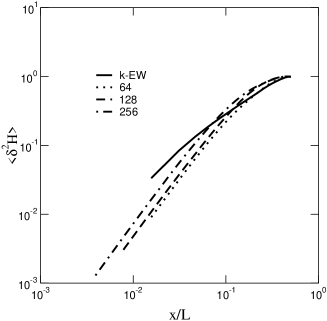
Figure 10: Amplitude of the interface fluctuations (normalized with $\delta H(x=L/2$) $\langle\delta^{2}H\rangle(x)$ in $1d$ for both the QEW and a thermal EW model with similar boundaries. The drive rate, for grains, $f=1/100$ for the former, for all the $L=64\dots 256$. [128]

5 SOC in the Kardar-Parisi-Zhang depinning

The second fundamental equation for depinning problems is the quenched Kardar-Parisi-Zhang one [129, 130],

$$\partial_{t}H({\bf x},t)=\nu\nabla^{2}H({\bf x},t)+\lambda(\nabla H({\bf x},t))^{2}+F+\eta(x,H(x,t)),$$ (51)

$\lambda$ measures the strength of the celebrated KPZ nonlinearity, proportional to the squared local interface slope [131]. The previous analysis of reaching a non-equilibrium critical steady-state can now be repeated in the presence of the $\lambda$-term, to study the difference between the QKPZ and the EW equations (a non-linear Langevin equation and a linear diffusion equation) [132]. The dynamics of the latter is insensitive to initial profiles (unless no other noise is present), while the QKPZ has a growth component $\partial_{t}H$ perpendicular to the interface slope, always non-zero.

The Eq. (51) suffers from the problem that it is notoriously hard to integrate numerically. Some discretizations exist, a reasonable example [133] is given by

$$f_{i}(t)=\nu\nabla^{2}H_{i}(t)+{\lambda\over 4}\left([H_{i}(t)-H_{i-1}(t)]^{2}+[H_{i+1}(t)-H_{i}(t)]^{2}\right)$$

$$+F(t)+\eta_{i,H_{i}}.$$ (52)

where $f_{i}(t)$ is again a local force. The QKPZ sandpile is such that a site gives $2\nu$ particles or units of energy to its neighbors once it topples, and the toppling criterion also compares the integrated activity at site $i$ to its neighbors. In the interface picture $H_{i}(t+1)=H_{i}(t)+\Theta(f_{i}(t))$. With this definition, $H(x,t)=\int^{t}\rho(x,\tau)d\tau$ maps the discrete QKPZ equation to the ’sandpile’ and vice versa. Now the simple dynamics $\partial_{t}H=\theta(f)$ and pinning boundary conditions $H=0$ at the boundaries imply a SOC ensemble, if $F(t)$ is ramped slowly as in usual sandpiles. Note that the exponents of the depinning transition depend on e.g. if $\lambda$ approaches zero with $\Delta F\equiv F-F_{c}\rightarrow 0$ (One can map a directed sandpile to the KPZ equation, without considering the history [134]).

The roughening, the development of average local slopes, depends on the sign of $\lambda$. If $F(t)>0$ the interface becomes unstable if $\lambda>0$. If $\lambda<0$ one can study a separation of time-scales: the system is driven so that $F(t)$ is increased after an avalanche has relaxed. Fig. 11 shows a series of snapshots from a simulation of the QKPZ equation with $\eta_{i,H_{i}}=\pm g$ with equal probability. This describes random toppling thresholds that change after each toppling in the sandpile language.

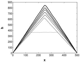
Figure 11: Typical interface configurations for a $1d$ QKPZ, with SOC drive and boundary conditions, for a system of 500 sites. The one with the flat top is an unstable one from the initial growth event before steady-state of the model, and the others are from every 20000th time step [132].

The shape of the interface is triangular in 1+1-D as expected with $\lambda<0$ (see also [135]). For a flat slope the surface tension is negligible, and a slope arises from the balance of the nonlinearity and the driving force, $\langle|\nabla h|\rangle=\sqrt{2\zeta t/\lambda}$. This is analogous to the development of the steady-state grain configuration in usual SOC. In the ensuing phase usual avalanche properties can be measured, eg. $\tau_{s}=2.5\pm 0.1$, implying that the average avalanche size is independent of $L$, contrary to usual sandpiles with anomalous diffusion, since $\tau_{s}>2$.

The avalanches are in addition time-translation invariant only on the average: the largest avalanches happen when the roughness of the interface is the largest. Local slopes, i. e. $|H_{i}-H_{i-1}|$ alternate between $n$ and $n+1$ where $n$ is a positive integer. In spite of such deterministic trends there is no characteristic avalanche size. Such dynamics (for the size, duration, and support) of avalanches eventually changes due to the development of a critical slope $m_{c}$. This is a signature of different effective dynamics of avalanches, above $m_{c}$, which one reaches in $L^{2}$ avalanches.

The combination of slow drive and boundary pinning eventually pick a symmetry for the average interface profile. Write the interface field on one of the sides of the triangle (1d) as $H(x,t)=m(t)x+\delta H(x,t)$. Inserting this into the QKPZ equation we obtain for $\delta H$

$${\partial\delta H({\mathbf{x}},t)\over\partial t}=\nu\nabla^{2}\delta H+{\lambda}m(t)\nabla\delta H+{\lambda\over 2}(\nabla\delta H)^{2}+\eta({\mathbf{x}},H),$$ (53)

subtracting the mean-field solution, valid for intermediate times $\delta t\ll t$. The effective interface equation has a linear term in $\nabla\delta H$, that will dominate over the KPZ-nonlinearity. This is a full analogy of depinning in the presence of anisotropic quenched noise [136], explaining the presence of this regime.

6 Conclusions and discussion

In this article we have outlined the connection of sandpile-like cellular automata, exhibiting “self-organized criticality”, to other non-equilibrium phase transitions. Such mappings allow to establish a number of facts about sandpiles, and leave a number of open questions.

The first observations concern the role of ensembles and rules. The mappings to interface depinning reveal, how SOC avalanche properties depend on the details of the SOC automaton. The connections to both absorbing state phase transitions and the depinning illuminate the role of history effects in sandpile dynamics. Below, a few evident conclusions are listed.

1. the noise in the LIM-representation settles the universality class, in the absence of strong additional symmetries (BTW model).

2. the upper critical dimension, in the presence of a surface tension, is four.

3. for non-SOC ensembles the critical exponent follow from the FES/depinning transition. In some cases these present an open problem, since the QEW with certain kinds of correlated noise is not well understood (in terms of $\chi$, $z$ etc.). This has not been resolved in the NDCF-picture either, due to the lack of analytical progress.

4. the derivation of the avalanche exponents for SOC sandpiles is an open problem. In some cases (Zhang, Manna/NDCF class) this can be directly traced to the fact that the noise of the interface equation becomes ${\bf x}$-dependent. Thus translational invariance is broken. The same holds for off-critical SOC sandpiles.

5. the off-critical models can still show criticality (eg. of the thermal EW-class)

6. temperature can be introduced easily [137], via the idea of adding “thermal noise” into the interface equation [138, 139], and interpreting it in the sandpile language.

7. the rule of conservation laws is highlighted (Laplacian operator, the FES class and its description via an activity picture).

8. the boundary conditions of the SOC ensemble may (QKPZ “sandpile”) lead to different dynamics, due to symmetry-breaking.

In summary, the existence of “SOC” is by such mappings revealed to be a result of combination of “non-linearity” (underlying ordinary non-equilibrium phase transition) together with a slow drive in an inhomogeneous system (net current of particles or energy). It is not an “attractive fixed point”, but arises from fine-tuning the drive rate so that avalanches separate.

One outcome is naturally the prospect of observing “true SOC” by preparing an experiment with boundary conditions that exactly correspond to what the theory would imply. Driven interfaces in random media (domain walls in random magnets, for instance) would seem to be an obvious candidate. Note that the predictions for open systems differ depending whether the system is exactly in the SOC state or not. Concerning theoretical aspects, the mapping of dynamics to a history description might be of advantage in other problems, like coupled map-lattices (for the contact process, e.g. a new exponent arises [140, 141]) and reaction-diffusion systems (eg. [142]).

For SOC-like cellular automata and their continuum descriptions one may list a number of open topics, including those related to the list above. Understanding the nature of the SOC ensemble; the origins of multiscaling therein; mapping depinning to absorbing state phase transitions [71] renormalization techniques for both depinning (in non-standard ensembles like the SOC, and with correlated noise) and the conserved field theory of NDCF models.

Other topics are the continuum descriptions of models with more complicated rules (curvature -dependent thresholds, like for sandpiles derived out of driven MHD equations [143], in both SOC and FES ensembles; the vortex flow model of Paczuski and Bassler that may be in the randomly boundary -driven columnar noise LIM-class [43], the non-local rules employed already by Kadanoff et al. [100] and so forth. In the interface context, the presence of long-range interactions substituting the Laplacian surface tension in Eq. (39) changes the scaling exponents [144]. For all such cellular automata one expects that they can be mapped to known continuum equations with quenched randomness, possibly with noise correlations. This also implies that e.g the predictability [145] of such SOC systems is very low and that the damage tolerance is high [146]. An analogy is provided by a percolation problem, in which one removes bonds around $p_{c}$ randomly till the spanning cluster is broken; then new ones are added again till a spanning cluster is re-formed. Clearly it is to first order difficult to “predict” whether the largest cluster is system-spanning or not and in fact the only information hidden in the behavior is the usual spanning probablity (vs. $p$).

Acknowledgments

I would like to acknowledge in particular Kent Lauritsen for collaborating on the connections between sandpiles and depinning, as well as all my other collaborators on such issues, including Miguel Muńoz, Romualdo Pastor-Satorras, Ron Dickman, Alessandro Vespignani, Amit Chattopadhyay, and Lasse Laurson. Stefano Zapperi is thanked for a pleasant stay in Rome, where this manuscript was being prepared, and the editors Elka and Rodolfo, for the possibility of contributing to the book. Also, Hugues Chaté is thanked for the data of Table 2. Financial support from SMC, La Sapienza, Rome, and the Center of Excellence program, Academy of Finland is also acknowledged.

References

- [1] P. Bak, C. Tang and K. Wiesenfeld, Phys. Rev. Lett. 59, 381 (1987); Phys. Rev. A38, 364 (1988); see also: P. Bak, How Nature Works (Copernicus, New York, 1996).
- [2] R. Dickman, M. A. Muñoz, A. Vespignani, and S. Zapperi, Braz. J. Phys. 30, 27 (2000); D. Dhar, Physica A 264, 1 (1999); H. J. Jensen, Self organized criticality, (Cambridge Univ. Press, Cambridge, 1998); R. Dickman, Physica A 306, 90 (2002).
- [3] J. Marro and R. Dickman, Nonequilibrium Phase Transitions in Lattice Models (Cambridge University Press, Cambridge, 1999).
- [4] O. Narayan and A. A. Middleton, Phys. Rev. B49, 244 (1994).
- [5] M. Paczuski and S. Boettcher, Phys. Rev. Lett. 77, 111 (1996).
- [6] M. Paczuski, S. Maslov, and P. Bak, Phys. Rev. E53, 414 (1996).
- [7] D. Cule and T. Hwa, Phys. Rev. B57, 8235 (1998).
- [8] M.J. Alava and K.B. Lauritsen, Europhys. Lett. 53, 563 (2001); see also cond-mat/9903349.
- [9] M. J. Alava, J. Phys. Cond. Mat. 14, 2353 (2002).
- [10] A. -L. Barabási and H. E. Stanley, Fractal Concepts in Surface Growth, (Cambridge University Press, Cambridge, 1995).
- [11] A. Diaz-Guilera, Phys. Rev. A45, 8551 (1992).
- [12] A. Díaz-Guilera, Europhys. Lett. 26, 177 (1994); L. Pietronero, A. Vespignani and S. Zapperi, Phys. Rev. Lett. 72, 1690 (1994); J. Hasty and K. Wiesenfeld, J. Stat. Phys. 86, 1179 (1997).
- [13] C. Tang and P. Bak, Phys. Rev. Lett. 60, 2347 (1988).
- [14] A. Vespignani and S. Zapperi, Phys. Rev. Lett. 78, 4793 (1997); Phys. Rev. E57, 6345 (1998).
- [15] S. S. Manna, J. Phys. A 24, L363 (1992); J. Stat. Phys. 59, 509 (1990).
- [16] Y. C. Zhang, Phys. Rev. Lett. 63, 470 (1989).
- [17] G. Grinstein, in Scale Invariance, Interfaces and Nonequilibrium Dynamics, NATO Advanced Study Institute, Series B: Physics, vol. 344, A. McKane et al., Eds. (Plenum, New York, 1995).
- [18] G. Grinstein, J. Appl. Phys. 69, 5441 (1991).
- [19] T. Hwa and M. Kardar, Phys. Rev. A45, 7002 (1992).
- [20] D. Sornette, A. Johansen, and I. Dornic, J. Phys. I (France) 5, 325 (1995).
- [21] D. Dhar, Physica A 263 (1999) 4 and references therein.
- [22] D.V. Ktitarev et al., Phys. Rev. E61, 81 (2000).
- [23] S.N. Majumdar and D. Dhar, Physica A 185, 129 (1992).
- [24] C. Tebaldi, M. DeMenech, and A. Stella, Phys. Rev. Lett. 83, 3952 (1999); M. de Menech, A.L. Stella, and C. Tebaldi, Phys. Rev. E58, R2677 (1998); M. De Menech, A. L. Stella, Phys. Rev. E62, R4528 (2000)
- [25] P. Bak and K. Sneppen, Phys. Rev. Lett. 71, 4083 (1993).
- [26] B. Drossel and F. Schwabl, Phys. Rev. Lett. 69, 1629 (1992).
- [27] S. Clar, B. Drossel and F. Schwabl, Phys. Rev. E50, 1009 (1994).
- [28] H. M. Jaeger, C. H.- Liu and S. R. Nagel, Phys. Rev. Lett. 62, 40 (1989).
- [29] H. M. Jaeger, S. R. Nagel and R. P. Behringer, Rev. Mod. Phys. 68, 1259 (1996).
- [30] V. Frette, K. Christensen, A.M. Malthe-Sørenssen, J. Feder, T. Jøssang and P.Meakin, Nature 397, 49 (1996).
- [31] C.M. Aegerter, M.S. Welling, and R.J. Wijngaarden, cond-mat/0305591.
- [32] H. Barkhausen, Z. Phys. 20, 401 (1919).
- [33] G. Bertotti, G. Durin, and A. Magni, J. Appl. Phys. 75, 5490 (1994).
- [34] G. Durin, G. Bertotti, and A. Magni, Fractals 3, 351 (1995).
- [35] D. Spasojević, S. Bukvić, S. Milosević, and H. E. Stanley, Phys. Rev. E54, 2531 (1996).
- [36] J. S. Urbach, R. C. Madison, and J. T. Markert, Phys. Rev. Lett. 75, 276 (1995).
- [37] S. Zapperi, P. Cizeau, G. Durin, and H. E. Stanley, Phys. Rev. B 58, 6353 (1998).
- [38] C. P. Bean, Rev. Mod. Phys. 36, 31 (1964).
- [39] C. Tang, Physica A 194, 315 (1993).
- [40] S. Field, J. Witt, F. Nori, and X. Ling, Phys. Rev. Lett. 74, 1206 (1995).
- [41] E. Altshuler et al. cond-mat/0208266
- [42] C.M. Aegerter, R. Günther, and R.J. Wijngaarden, cond-mat/0305592.
- [43] K. E. Bassler and M. Paczuski, Phys. Rev. Lett. 81, 3761 (1998); K. E. Bassler, M. Paczuski, and G.F. Reiter Phys. Rev. Lett. 83, 3956 (1999);
- [44] M. Nicodemi and H.J. Jensen, J. Phys. A 34, L11 (2001).
- [45] C. J. Olson, C. Reichhard and F. Nori, Phys. Rev. B56, 6175 (1997);
- [46] A. Garcimartín, A. Guarino, L. Bellon and S. Ciliberto, Phys. Rev. Lett. 79, 3202 (1997); A. Guarino, A. Garcimartín and S. Ciliberto, Eur. Phys. J. B 6, 13 (1998).
- [47] L.I. Salminen, A.I. Tolvanen, and M.J. Alava, Phys. Rev. Lett. 89, 185503 (2002).
- [48] A. Petri, G. Paparo, A. Vespignani, A. Alippi and M. Costantini, Phys. Rev. Lett. 73, 3423 (1994).
- [49] D. L. Turcotte, Rep. Prog. Phys. 62, 1377 (1999).
- [50] J. Weiss and. J.-R. Grasso, J. Phys. Chem. B 101, 6113 (1997).
- [51] J. Weiss and D. Marsan, Science 299 89 (2003).
- [52] P. Charbonneau et al., Solar Phys. 203, 321 (2001).
- [53] S. Chapman and N. Watkins, Space Sci. Rev. 95, 293 (2001).
- [54] G. Consolini and T.S Chang, Space Sci. Rev. 95, 309 (2001).
- [55] Physics of Plasmas 6, November issue (1999).
- [56] R.O. Dendy and P. Helander, Plasma Phys. Contr. Fusion, 39, 1947 (1997).
- [57] E.T. Lu and R.J. Hamilton, Astrophys. J. 380, L89 (1991); E.T. Lu, R.J. Hamilton, J.M. McTiernan, and K.R. Bromund, Astrophys. J. 412, 841 (1993).
- [58] H. Leschhorn, Physica A 195, 324 (1993).
- [59] O. Narayan and D. S. Fisher, Phys. Rev. B48, 7030 (1993).
- [60] T. Nattermann et al., J. Phys. (France) II 2, 1483 (1992); H. Leschhorn et al. Ann. Physik 7, 1 (1997).
- [61] H. Hinrichsen, Adv. Phys. 49, 1, (2000).
- [62] M. Rossi, R. Pastor-Satorras, and A. Vespignani, Phys. Rev. Lett. 85, 1803 (2000).
- [63] R. Pastor-Satorras, and A. Vespignani, Phys. Rev. E62, 5875 (2000).
- [64] M. A. Muñoz, R. Dickman, R. Pastor-Satorras, A. Vespignani, and S. Zapperi, Sandpiles and absorbing state phase transitions: recent results and open problems, in ”Modeling Complex Systems”, Ed. J. Marro and P. L. Garrido. AIP Conference Proceedings, vol. 574, 102 (2001).
- [65] S. Lübeck, Phys. Rev. E66 046114, (2002); S. Lübeck and A. Hucht, J. Phys. A 34, L577 (2001).
- [66] M. Doi, J. Phys. A 9, 1465 (1976); L. Peliti, J. Phys. I 46, 1469 (1985); B. P. Lee and J. L. Cardy J. Stat. Phys. 80, 971 (1995).
- [67] F. van Wijland, K. Oerding, and H. J. Hilhorst, Physica A 251, 179 (1998). See also R. Kree, B. Schaub, and B. Schmittmann, Phys. Rev. A 39, 2214 (1989).
- [68] R. Dickman, A. Vespignani, and S. Zapperi, Phys. Rev. E57, 5095 (1998); A. Vespignani et al., Phys. Rev. Lett. 81, 5676 (1999).
- [69] H. K. Janssen, Z. Phys. 42, 141 (1981); ibid. 58, 311 (1985); P. Grassberger, Z. Phys. B 47, 465 (1982); Cardy J.L., Sugar R.L. (1980), J. Phys. A 13, L423.
- [70] F. van Wijland, Phys. Rev. Lett. 89, 190602 (2002).
- [71] M. Alava and M.A. Muñoz, Phys. Rev. E65, 026145 (2002)
- [72] T. Halpin-Healy and Y.-C. Zhang, Phys. Rep. 254, 215 (1995).
- [73] P. Meakin, Fractals, scaling and growth far from equilibrium (Cambridge Univ. Press, Cambridge, 1998).
- [74] D. Sornette, Critical Phenomena in Natural Sciences (Springer, Berlin, 2000).
- [75] J. Krug, Phys. Rev. Lett. 72, 2907 (1994).
- [76] J. Asikainen, S. Majaniemi, M. Dube, and T. Ala-Nissila, Phys. Rev. E65, 052104 (2002).
- [77] S.J. Mitchell, cond-mat/0210239.
- [78] J.M. L\a’opez, M.A. Rodr\a’ıguez, and R. Cuerno, Phys. Rev.
- [79] J.M. López, Phys. Rev. Lett. 83, 4594 (1999).
- [80] H. Leschhorn and L.-H. Tang, Phys. Rev. Lett. 70, 2973 (1993).
- [81] H. Leschhorn and L.H. Tang, Phys. Rev. E49, 1238 (1994).
- [82] H. Leschhorn, Phys. Rev. E54, 1313 (1996).
- [83] P. Chauve, P. Le Doussal, and K. Wiese, Phys. Rev. Lett. 86, 1785 (2001); P. Le Doussal, K.J. Wiese, and P. Chauve, Phys. Rev. B66, 174201 (2002).
- [84] A. Rosso and W. Krauth, Phys. Rev. Lett. 87 (2001) 187002.
- [85] O. Narayan, Phys. Rev. E62, R7563 (2000).
- [86] See e.g. F. Lacombe, S. Zapperi and H. J. Herrmann, Phys. Rev. B63, 104104 (2001).
- [87] K. Christensen et al., Phys. Rev. Lett. 77, 107 (1996).
- [88] G. Pruessner, Phys. Rev. E67, 0303301 (2003).
- [89] Z. Olami et al., Phys. Rev. Lett. 68, 1244 (1992).
- [90] M. Marsili, J. Stat. Phys. 77, 733 (1994).
- [91] J. Kockelkoren and H. Chaté, cond-mat/0306039.
- [92] R. Dickman, Europhys. Lett. 61, 294 (2003).
- [93] P.K. Mohanty and D. Dhar, Phys. Rev. Lett. 89, 104303 (2002); A. Vazquez and O.Sotolongo-Costa, Phys. Rev. E61, 944 (2000); A. Vazquez and O.Sotolongo-Costa, J. Phys. A 32, 2633 (1999).
- [94] T.J. daSilva and J.G. Moreira, Phys. Rev. E56, 4880 (1997).
- [95] A. Chessa, E. Marinari, and A. Vespignani, Phys. Rev. Lett. 80, 4217 (1998).
- [96] A. Vespignani, R. Dickman, M. A. Muñoz, and S. Zapperi, Phys Rev. E62, 4564 (2000); R. Dickman et al. Phys. Rev. E64, 056104 (2001).
- [97] F. Bagnoli et al., cond-mat/0207674.
- [98] A. Barrat, A. Vespignani, and S. Zapperi, Phys. Rev. Lett. 83, 1962 (1999).
- [99] D. Dhar, Phys. Rev. Lett. 64, 1613 (1990).
- [100] L. P. Kadanoff et al., Phys. Rev. A39, 6524 (1989).
- [101] A. Montakhab and J.M. Carlson Phys. Rev. E58, 5608 (1998); J.M. Carlson et al., Phys. Rev. E48, 688 (1993).
- [102] A. Chessa et al., Phys. Rev. E59, R12 (1999).
- [103] O. Biham, E. Milshtein, and O. Malcai, Phys. Rev. E63, 061309 (2001).
- [104] A. Ben-Hur and O. Biham, Phys. Rev. E53, R1317 (1996).
- [105] B. Drossel, Phys. Rev. E61, R2168 (2000).
- [106] V.B. Priezzhev, E.V. Ivashkevich, and D.V. Ktitarev, Phys. Rev. Lett. 76, 2093 (1996); D.V. Ktitarev and V.B. Priezzhev, Phys. Rev. E58 2883 (1998).
- [107] M. Paczuski and S. Boettcher, Phys. Rev. E57, R3745 (1997).
- [108] S. Lübeck, Phys. Rev. E62, 6149 (2000).
- [109] R. Pastor-Satorras and A. Vespignani, Eur. Phys. J. B18, 197 (2001).
- [110] R. Pastor-Satorras and A. Vespignani, Eur. Phys. J. B19, 583 (2001).
- [111] R. Dickman and J. M. M. Campelo, cond-mat/0301054.
- [112] H. A. Makse et al., Europhys. Lett. 41, 251 (1998).
- [113] G. Huber, M.H. Jensen, and K. Sneppen, Phys. Rev. E52, R2133 (1995).
- [114] Z. Olami, I. Procaccia, and R. Zeitak, Phys. Rev. E52, 3042 (1995).
- [115] M. Jost, Phys. Rev. E57, 2634 (1998).
- [116] A.-L. Barabasi, G. Grinstein, and M. Muńoz, Phys. Rev. Lett. 76, 1481 (1996).
- [117] M. Howard, P. Frojdh, and K. Bækgaard Lauritsen, Phys. Rev. E61, 167 (2000).
- [118] G. Parisi and L. Pietronero, Europhys. Lett. 16, 321 (1991); Physica A 179, 16 (1991).
- [119] A. Vazquez, Phys. Rev. E62, 7797 (2000); T. Tsuchiya and M. Katori, Phys. Rev. E61, 1183 (2000).
- [120] G. Miller and C. J. Boulter, Phys. Rev. E67, 046114 (2003); B. Drossel, Phys. Rev. Lett. 89, 238701 (2002); M. de Sousa Vieira, Phys. Rev. E66, 051306 (2002); G. Miller and C. J. Boulter, Phys. Rev. E66, 016123 (2002); S. Lise and M. Paczuski, Phys. Rev. E66, 046111 (2001).
- [121] A. Corral and M. Paczuski, Phys. Rev. Lett. 83, 572 (1999).
- [122] P. de los Rios and Y.-C. Zhang, Phys. Rev. Lett. 82, 472 (1999).
- [123] J. Krug, Phys. Rev. A44, R801 (1991).
- [124] A. Giacometti and A. Diaz-Guilera, Phys. Rev. E58, 247 (1998); B. Kutnjak-Urbanc, S. Havlin, and H.E. Stanley, Phys. Rev. E54, 6109 (1996).
- [125] N.-N. Pang and N. Y. Liang Phys. Rev. E56, 1461 (1997).
- [126] L. Laurson and M.J. Alava, submitted for publication.
- [127] A. Baldassari, F. Colaiori, and C. Castellano, Phys. Rev. Lett. 90, 060601 (2003).
- [128] M.J. Alava and A. Kr. Chattopadhyay, submitted for publication.
- [129] L.-H- Tang and H. Leschhorn, Phys. Rev. A45, R8309 (1992); S. Buldyrev et al. Phys. Rev. A45, R8313 (1992); Z. Olami, I. Procaccia, and R. Zeitak, Phys. Rev. E49, 1232 (1994).
- [130] N. Neshkov, Phys. Rev. E61, 6023 (2002).
- [131] M. Kardar, G. Parisi, and Y.-C. Zhang, Phys. Rev. Lett. 56, 889 (1986).
- [132] G. J. Szabo, M. J. Alava, and J. Kertesz, Europhys. Lett. 57, 665 (2002).
- [133] T.J. Newman and A.J. Bray, J. Phys A 29, 7917 (1996).
- [134] C.C. Chen and M. den Nijs, Phys. Rev. E65, 031309 (2002).
- [135] F. de los Santos, M.M. Telo da Gama, and M.A. Muñoz, Europhys. Lett. 57, 803 (2002).
- [136] L.-H. Tang, M. Kardar, and D. Dhar, Phys. Rev. Lett. 74, 920 (1995).
- [137] G. Caldarelli, Physica A 252, 295 (1998).
- [138] P. Chauve, T. Giamarchi, and P. Le Doussal, Phys. Rev. B63, 6241 (20001).
- [139] L. Roters, S. Lübeck, and K.D. Usadel, Phys. Rev. E63, 026113 (2001); L. Roters et al., Phys. Rev. E60, 5202 (1999).
- [140] R. Dickman and M. A. Muñoz, Phys. Rev. E62, 7632 (2000).
- [141] A. P. F. Atman, R. Dickman, and J.G. Moreira, Phys. Rev. E67 016107, (2003); A. P. F. Atman, R. Dickman, and J.G. Moreira, Phys. Rev. E66 016113, (2002); A. P. F. Atman and J. G. Moreira, Eur. Phys. J. B 16 (2000) 501; J. A. deSales, M.L. Martins, and J.G. Moreira, Physica A 245, 461 (1997).
- [142] A. Carpio, L. L. Bonilla, A. Luzon, Phys. Rev. E65, 035207(R) (2002).
- [143] H.-L. Liu et al. Phys. Rev. E66, 056111 (2002).
- [144] A. Tanguy, M. Gounelle, and S. Roux, Phys. Rev. E58, 1577 (1999).
- [145] S. L. Pepke and J. M. Carlson Phys. Rev. E50, 236 (1994).
- [146] M. Stapleton, M. Dingler, and K. Christensen, cond-mat/0306647.