Dynamical correlations in multiorbital Hubbard models: Fluctuation-exchange approximations

Abstract

We study the two band degenerate Hubbard model using the Fluctuation Exchange approximation (FLEX) and compare the results with quantum Monte Carlo (QMC) calculations. Both the self-consistent and the non-self-consistent versions of the FLEX scheme are investigated. We find that, contrary to the one-band case, in the multiband case, good agreement with the quantum Monte Carlo results is obtained within the electron-electron $T$-matrix approximation using the full renormalization of the one-particle propagators. The crossover to strong coupling and the formation of satellites is more clearly visible in the non-self-consistent scheme. Finally we discuss the behavior of the FLEX for higher orbital degeneracy.

1 Introduction

Recent progress in the development and application of advanced experimental techniques made available a number of new materials and compounds with strongly correlated electrons that cannot be entirely described within the Density Functional Theory (DFT) [1, 2]. Some transition-metal alloys, cuprates, manganites, heavy-fermion Kondo and mixed-valence systems, as well as lanthanides and transuranium compounds behave in a way that can neither be explained nor understood within first-principles computational schemes based on local approximations of the correlation-exchange potential in the DFT. It is necessary to take explicitly into account dynamical fluctuations to describe these materials. It can be done at best and in a manageable way within the Dynamical Mean Field Theory (DMFT) [3]. The DMFT captures most of the relevant local quantum dynamical effects of electron correlations. Recent progress in the development of various impurity solvers for the DMFT has opened a way for combining advanced many-body techniques with ab initio methods to build realistic computational schemes for materials with strongly correlated electrons.

The standard way of combining ab initio calculations with the DMFT is via multiorbital Hubbard models. The input parameters for multiorbital Hubbard models to be solved within the DMFT are determined from ab initio calculations, for example using the linearized muffin-tin orbital (LMTO) method [4]. No universal scheme to solve the DMFT equations exactly does exist. Hence, one has to resort to approximate impurity solvers to reach quantitative results from the DMFT. We distinguish essentially two types of DMFT solvers: numerical schemes and analytical methods based on many-body perturbation theory. The former schemes aim at numerically exact quantitative solutions while the latter at analytically controllable schemes. Although analytic methods are not quantitatively as accurate as the numerical solutions, they have an appealing feature in that they offer an analytically controllable approach with a direct access to spectral functions on the real frequency axis. Analytic approaches are needed in most situations to complement the numerical solutions so that we can assess the peak structure of spectral functions when performing analytic continuation of numerical results from the imaginary axis of Matsubara frequencies. To gain confidence in approaches based on many-body perturbation theory we should test them in simpler situations and compare their results with available more precise numerical simulations.

In the context of the one-band model, extensive comparisons between perturbative approaches such as the the Iterated Perturbation Theory (IPT) and the QMC method have been carried out (see, for example, Refs. [5, 3]). It appeared that the non-self-consistent IPT is a rather accurate approximation. Analytic extension of the IPT and second-order perturbation theory via multiple two-particle scatterings, the FLEX, has already been applied to iron and nickel in self-consistent and non-self-consistent forms.[6, 7] However, a critical discussion of accuracy of this method in multi-band situation and comparison with e.g. QMC have not yet been carried out. It is the aim of this paper to fill this void, and compare diagrammatic schemes with dynamical fluctuations based on two-particle scatterings with finite-temperature quantum Monte Carlo solution of the DMFT. To this end we use a multiorbital Hubbard model with a simplified kinetic energy so that we can focus our attention on the fundamental features of the transition between weak and strong electron couplings in multiorbital Hubbard models.

A typical form of the Hamiltonian used in dynamical extensions of DFT schemes is

$$H^{\rm Hubb} = \sum_{{\bf R}\lambda,{\bf R^{\prime}}\lambda^{\prime}}t_{{\bf R}\lambda,{\bf R^{\prime}}\lambda^{\prime}}\,a^{+}_{{\bf R}\lambda}\,a_{{\bf R^{\prime}}\lambda^{\prime}}$$

$$+ \sum_{{\bf R},\lambda,\lambda^{\prime}\lambda^{\prime\prime}\lambda^{\prime\prime\prime}}\langle{\bf R}\lambda,{\bf R}\lambda^{\prime}|V|{\bf R}\lambda^{\prime\prime}{\bf R}\lambda^{\prime\prime\prime}\rangle\,a^{+}_{{\bf R}\lambda}a^{+}_{{\bf R}\lambda^{\prime}}a_{{\bf R}\lambda^{\prime\prime\prime}}a_{{\bf R}\lambda^{\prime\prime}},$$

where $\mathbf{R}$ are lattice site coordinates and $\lambda=(l\sigma)$ are spin-orbital indices. The hopping term $t_{{\bf R}\lambda,{\bf R^{\prime}}\lambda^{\prime}}$ is determined from ab initio electronic structure calculations and will be replaced in this comparison study with a model dispersion relation diagonal in the spin-orbital indices. The electron interaction is usually considered only between the $d$-electrons, since the effect of the lower orbitals is assumed to be described quite well within the standard DFT. We assume that the local interaction consists only of direct and exchange terms. We approximate the interaction operator with two parameters only: the Hubbard $U$ and the exchange constant $J$. In homogeneous cases (without disorder) we can neglect the lattice coordinate and represent the interaction only with a quadruple of spin-orbital indices

$$\langle i\sigma j\sigma^{\prime}|V|k\sigma l\sigma^{\prime}\rangle\,\approx\delta_{ik}\delta_{jl}(1-\delta_{ij}\delta_{\sigma\sigma^{\prime}})\,U+\delta_{il}\delta_{jk}(1-\delta_{ij})\delta_{\sigma\sigma^{\prime}}\,J\,.$$ (2)

This representation can easily be further simplified to a standard matrix in the spin-orbital indices

$$v_{\lambda\lambda^{\prime}}=(1-\delta_{\lambda\lambda^{\prime}})(U-J\delta_{\sigma\sigma^{\prime}})\ .$$ (3)

We use this representation of the electron interaction in our many-body treatment of the multiorbital Hubbard model.

2 Methods

2.1 Many-body dynamical fluctuations

The effects of the electron interaction on one-particle states are described by the self-energy $\Sigma_{\lambda}$. Dynamical fluctuations are contained in the two-particle vertex function $\Gamma_{\lambda\lambda^{\prime}}$. We denote four-momenta $k=(\mathbf{k},i\omega_{n})$ and $q=(\mathbf{q},i\nu_{m})$, and use the Schwinger-Dyson equation to relate the two-particle vertex with the one-particle self-energy. With representation (3) for the electron interaction we can write

$$\Sigma_{\lambda}(k) = \sum_{\lambda^{\prime}}\frac{1}{\beta N}\sum_{k^{\prime}}v_{\lambda\lambda^{\prime}}G_{\lambda^{\prime}}(k^{\prime})\times$$

$$\left[1-\frac{1}{\beta N}\sum_{q}G_{\lambda}(k-q)G_{\lambda^{\prime}}(k^{\prime}-q)\Gamma_{\lambda\lambda^{\prime}}(k-q;q,k^{\prime}-k)\right]\ .$$

The first term on the r.h.s. of Eq. (2.1) is the static Hartree term expressing the self-energy in terms of densities. This term in realistic calculations is normally part of the static local density approximation fixing the static particle densities. We hence suppress the Hartree term and use only the vertex contribution to the self-energy as a generator of dynamical fluctuations missing in the DFT.

The simplest approximation on the vertex function $\Gamma_{\lambda\lambda^{\prime}}$ is the bare interaction $v_{\lambda\lambda^{\prime}}$. Such an approximation corresponds to second-order perturbation theory (SOPT). The vertex is momentum independent. Even in more advanced approximations we will not use the full momentum dependence of the vertex function. In our treatment we resort only to multiple scatterings of two quasiparticles (FLEX) [8]. In this situation the two-particle vertex depends on only a single bosonic four-momentum $q$. This dependence enters the vertex function via a two-particle bubble. When we deal with multiple electron-hole scatterings the bubble is

$$\Phi_{\lambda\lambda^{\prime}}(q)=\frac{1}{\beta N}\sum_{k}G_{\lambda}(k)G_{\lambda^{\prime}}(k+q)\ .$$ (5)

The self-energy due to dynamical electron-hole (multiple) scatterings can then be represented as

$$\Sigma^{eh}_{\lambda}(k)=\sum_{\lambda^{\prime}}\frac{1}{\beta N}\sum_{q}v_{\lambda\lambda^{\prime}}G_{\lambda^{\prime}}(k+q)\Phi_{\lambda\lambda^{\prime}}(q)\Gamma^{eh}_{\lambda\lambda^{\prime}}(q)\ .$$ (6)

In second-order perturbation theory $\Gamma^{eh}_{\lambda\lambda^{\prime}}=v_{\lambda\lambda^{\prime}}$. When we sum ladder electron-hole diagrams we obtain for the vertex function the following representation

$$\Gamma^{eh}_{\lambda\lambda^{\prime}}(q)=\frac{v_{\lambda\lambda^{\prime}}}{1+v_{\lambda\lambda^{\prime}}\Phi_{\lambda\lambda^{\prime}}(q)}\ .$$ (7)

To visualize the above equations we show corresponding diagrams for the vertex $\Gamma^{eh}$ of the particle–particle type shown in the top row of Fig. 1 and the corresponding contribution to the self-energy is shown in the bottom row of Fig. 1. Note that a small square in all diagrams (Fig. 1 – 3) represents the antisymmetrized pair interaction (cf. Ref. [9]).

Figure 1: Particle–hole (top row) vertex $\Gamma^{eh}$ which appears in the FLEX approximation. Definition of the FLEX self–energy constructed with the help of the particle–hole vertex (bottom row).

Analogously we can construct an approximation with multiple electron-electron scatterings where the self-energy can be represented as

$$\Sigma^{ee}_{\lambda}(k)=\sum_{\lambda^{\prime}}\frac{1}{\beta N}\sum_{q}v_{\lambda\lambda^{\prime}}G_{\lambda^{\prime}}(q-k)\Psi_{\lambda\lambda^{\prime}}(q)\Gamma^{ee}_{\lambda\lambda^{\prime}}(q)\ .$$ (8)

Here we have to use a particle-particle bubble

$$\Psi_{\lambda\lambda^{\prime}}(q)=\frac{1}{\beta N}\sum_{k}G_{\lambda}(k)G_{\lambda^{\prime}}(q-k)\ .$$ (9)

The two-particle vertex $\Gamma^{ee}_{\lambda\lambda^{\prime}}$ has the same solution as the electron-hole scattering function, Eq. (7), where only we replace the bubble $\Phi$ with $\Psi$. Corresponding set of diagrams for the vertex $\Gamma^{ee}$ and the self-energy is presented in Fig. 2.

Figure 2: Particle–particle (top row) vertex $\Gamma^{ee}$ which appears in the FLEX approximation. Definition of the FLEX self–energy constructed with the help of the particle–particle vertex (bottom row).

The third channel of two-particle scatterings is the interaction channel where the electron interaction is screened by electron-hole polarization bubbles. The dynamical self-energy due to this renormalization is then represented as

$$\Sigma^{v}_{\lambda}(k)=\sum_{\lambda^{\prime}}\frac{1}{\beta N}\sum_{q}v_{\lambda\lambda^{\prime}}G_{\lambda^{\prime}}(k+q)\Phi_{\lambda\lambda^{\prime}}(q)\Gamma^{v}_{\lambda\lambda^{\prime}}(q),$$ (10)

with

$$\Gamma^{v}_{\lambda\lambda^{\prime}}(q)=v_{\lambda\lambda^{\prime}}-\sum_{\lambda^{\prime\prime}}v_{\lambda\lambda^{\prime\prime}}\Phi_{\lambda^{\prime\prime}\lambda^{\prime\prime}}(q)\Gamma^{v}_{\lambda^{\prime\prime}\lambda^{\prime}}(q)\ .$$ (11)

Corresponding diagrams are presented in Fig. 3.

Figure 3: Particle–hole vertex $\Gamma^{v}$ corresponding to the third scattering channel is given in top row. Definition of the corresponding self–energy is presented in the bottom row.

We can treat each channel independently or add all three channels to assess the effect of dynamical fluctuations on the electron self-energy. In the latter case, however, we have to subtract twice the contribution from second order, since it is identical in all three channels.

The idea of the DMFT is to neglect the momentum dependence of the one-electron propagators in the contributions to the self-energy. We hence use only the local parts of the one-electron propagators, i. e., $G_{\lambda}(\mathbf{k},i\omega_{n})\to N^{-1}\sum_{\mathbf{k}}G_{\lambda}(\mathbf{k},i\omega_{n})=G_{\lambda}(i\omega_{n})$. Then, all the above formulas hold with the replacements $k\to i\omega_{n}$, $q\to i\nu_{m}$ for fermionic and bosonic momenta, respectively.

The advantage of analytic approaches with multiple two-particle scatterings is the knowledge of the explicit analytic structure of the self-energy. Hence all the above results can be explicitly analytically continued to real frequencies using a straightforward procedure. We explicitly mention only the result for the two-particle electron-hole bubble

$$\Phi_{\lambda\lambda^{\prime}}(z)=-\int_{-\infty}^{\infty}\frac{d\omega}{\pi}f(\omega-\mu)\left[G_{\lambda^{\prime}}(\omega+z){\rm Im}G_{\lambda}(\omega_{+})+G_{\lambda}(\omega-z){\rm Im}G_{\lambda^{\prime}}(\omega_{+})\right]\ .$$ (12)

Up to now we have used the fully renormalized one-electron propagators in the perturbation theory as demanded by conservation laws. However, when we are interested in the one-electron properties of the system, we can relax the demands of thermodynamic consistence and replace the fully renormalized propagator with a partially renormalized one

$$G^{-1}(z)\longrightarrow\mathcal{G}_{0}^{-1}(z)=G^{-1}(z)+\Sigma(z)+\tilde{\mu},$$ (13)

where in the expression for $G_{0}$ we used an additional shift of the impurity level to satisfy Luttinger’s theorem following Ref. [10]. This propagator goes over into the bare propagator in the atomic limit and does not contain long energy tails due to frequency convolutions in the definition of the self-energy.

This partially non-self-consistent scheme resembles IPT. Hence a better description of the transition from weak to strong coupling regimes at the one-particle level, including the metal-insulator transition (MIT), is expected from the IPT than from the conserving scheme with fully renormalized propagators, where the metal-insulator transition at half filling is known to be missing.

2.2 The quantum Monte Carlo

Among many methods used to solve the impurity problem we choose the quantum Monte Carlo method [11] to benchmark FLEX as a potential candidate for impurity solver. There are well known advantages and disadvantages of the QMC method and our choice is spurred by the fact that despite being slower than other methods, the QMC is well controlled, numerically exact method. As an input the QMC procedure gets Weiss function ${\cal G}_{0}(\tau)$ and as an output it produces Green’s function $G(\tau)$. We remind the reader major steps taken in the QMC procedure. Usually one starts with an impurity effective action $S$:

$$S_{\rm eff}=-\int^{\beta}_{0}d\tau d\tau^{\prime}\sum_{\alpha}c^{+}_{\alpha}(\tau){{\cal G}_{0}}_{\alpha}^{-1}(\tau,\tau^{\prime})c_{\alpha}(\tau^{\prime})+\frac{1}{2}\,\int^{\beta}_{0}d\tau\,\sum_{\alpha,\alpha^{\prime}}U_{\alpha\alpha^{\prime}}n_{\alpha}(\tau)n_{\alpha^{\prime}}(\tau),$$ (14)

where $\{c,\ c^{+}\}$ are fermionic annihilation and creation operators of the lattice problem, $\alpha=\{m,\sigma\}$.

The first what we should do with the action (14) is to discretize it in imaginary time with time step $\Delta\tau$ so that $\beta=L\Delta\tau$, and $L$ is the number of time intervals:

$$S_{\rm eff}\rightarrow\sum_{\alpha,\tau\tau^{\prime}}c_{\alpha}^{+}(\tau){{\cal G}_{0}}_{\alpha}^{-1}(\tau,\tau^{\prime})c_{\alpha}(\tau^{\prime})+\frac{1}{2}\sum_{\alpha,\alpha^{\prime}}U_{\alpha\alpha^{\prime}}n_{\alpha}(\tau)n_{\alpha^{\prime}}(\tau).$$ (15)

The next step is to get rid of the interaction term $U$ by substituting it by summation over Ising-like auxiliary fields. The decoupling procedure is called the Hubbard-Stratonovich transformation [12, 13]:

$$\exp\{-\Delta\tau\{U_{\alpha\alpha^{\prime}}n_{\alpha}n_{\alpha^{\prime}}-\frac{1}{2}(n_{\alpha}+n_{\alpha^{\prime}})\}\}=\frac{1}{2}\sum\limits_{S_{\alpha\alpha^{\prime}}=\pm 1}{}\exp\{\lambda_{\alpha\alpha^{\prime}}S_{\alpha\alpha^{\prime}}(n_{\alpha}-n_{\alpha^{\prime}})\},$$ (16)

where $\cosh\lambda_{\alpha\alpha^{\prime}}=\exp(\frac{{\Delta\tau U_{\alpha\alpha^{\prime}}}}{2})$ and $S_{\alpha\alpha^{\prime}}(\tau_{l})$ are auxiliary Ising fields at each time slice.

In the one-band Anderson impurity model we have only one auxiliary Ising field $S(\tau_{l})=\pm 1$ at each time slice, whereas in the multiorbital case number of auxiliary fields is equal to the number of $\alpha,\alpha^{\prime}$ pairs. Applying the Hubbard-Stratonovich transformation at each time slice we bring the action to a quadratic form with the partition function:

$$Z={\rm Tr}_{\{S_{\alpha\alpha^{\prime}}(\tau)\}}\prod_{\alpha}\det G^{-1}_{\alpha,\{S_{\alpha\alpha^{\prime}}(\tau)\}}\;,$$ (17)

where the Green function in terms of auxiliary fields $G^{-1}_{\alpha}$ reads

$$G^{-1}_{\alpha,\{S_{\alpha\alpha^{\prime}}\}}(\tau,\tau^{\prime})={{\cal G}_{0}}^{-1}_{\alpha}(\tau,\tau^{\prime})e^{V}-(e^{V}-1)\delta_{\tau,\tau^{\prime}},$$ (18)

with the interaction matrix

$$V_{\tau}^{\alpha}=\sum\limits_{\alpha^{\prime}(\neq\alpha)}\lambda_{\alpha\alpha^{\prime}}{S_{\alpha\alpha^{\prime}}(}\tau)\sigma_{\alpha\alpha^{\prime}},$$ (19)

where
$\sigma_{\alpha\alpha^{\prime}}=+1$ for $\alpha<\alpha^{\prime}$
$\sigma_{\alpha\alpha^{\prime}}=-1$ for $\alpha>\alpha^{\prime}$.

Once the quadratic form is obtained one can apply Wick’s theorem at each time slice and perform the Gaussian integration in Grassmann variables to get the full interacting Green function:

$$\!\!\!\!\!\!\!\!G_{\alpha}(\tau,\tau^{\prime})={\frac{{1}}{{Z}}}\,{\rm Tr}_{\{S_{\alpha\alpha^{\prime}}\}}G_{\alpha,\{S_{\alpha\alpha^{\prime}}\}}(\tau,\tau^{\prime})\prod_{\alpha^{\prime}}\det G^{-1}_{\alpha^{\prime},\{S_{\alpha\alpha^{\prime}}\}}.$$

To evaluate summation in Eq. (2.2) one uses Monte Carlo stochastic sampling. The product of determinants is interpreted as the stochastic weight and auxiliary spin configurations are generated by a Markov process with probability proportional to their statistical weight. More rigorous derivation can be find elsewhere  [3], [13].

Since the QMC method produces results in imaginary time axis ($G(\tau_{m})$ with $\tau_{m}=m\Delta\tau$, $m=1...L$) and the DMFT self-consistency equations make use of the frequency dependent Green’s functions and self-energies we must have an accurate method to compute Fourier transforms from the time to the frequency domain. This is done by representing the functions in the time domain by a cubic splined functions which should go through original points with condition of continuous second derivatives imposed. Once we know cubic spline coefficients we can compute the Fourier transformation of the splined functions analytically.

3 Results and Discussion

To compare analytic solutions with numerical ones we employed a simple model with two degenerate bands, i.e., four spin-orbitals per site and assumed a semi-elliptic density of states (DOS), $\rho_{0}(E)=\frac{2}{\pi}\sqrt{1-E^{2}}$. For simplicity we resorted to the case $J=0$ and non-magnetic solutions. We tested second-order perturbation theory together with multiple scatterings from the electron-hole and electron-electron interaction channels. Both types of self-consistency were considered, i. e., the full conserving and the partial one with the bath function $\mathcal{G}_{0}$, defined in the IPT Eq. (13). All approximations were analytically continued to real frequencies before being evaluated numerically. Maximum entropy method was used for analytical continuation to real axis. We tested maximum entropy method against other high-frequency more reliable methods like non-crossing approximation and one-crossing approximation and found satisfactory agreement understandable within limitations of all used methods. A simple iteration procedure with a suitably chosen mixing of the old and new self-energy led to well converged results for moderate values of the pair interaction $U$. The details of the numerical implementation of multiorbital FLEX-type approximations were described elsewhere [6, 7, 14, 15, 16].

First, we compared the analytical approximations among themselves for an intermediate value of the interaction strength, $U=2$. All energies are given in units of the half-bandwidth of the non-interacting DOS, $D=1$. We also wrote two different FLEX programs on real and imaginary axes and used 9000 and 4096 points on corresponding frequency domain with large enough frequency cut-off ($10D$) for temperature $T=1/16~{}D$. Using the conserving full self-consistence we found that results of SOPT and the electron-electron $T$-matrix approximation TMA are quite close to each other. The addition of the electron-hole TMA channel changes the result significantly. The quasiparticle width gets substantially reduced as shown in figure 4. This strong band narrowing is unphysical. We did not include the third channel, screening by the electron-hole polarization bubbles, explicitly to this figure, since it contributes quantitatively and qualitatively similarly to the electron-hole ladder. The reason why the electron-hole scatterings do not improve upon second order is quite clear. At the mean-field level an instability towards the local moment state with non-zero $\langle n_{\uparrow}\rangle-\langle n_{\downarrow}\rangle$ appears at some critical interaction. This instability is totally artificial because the conduction electrons screen the local moment (Kondo effect). In the non-self-consistent FLEX approach including both electron-electron and electron-hole TMA, this instability also occurs when the denominator in the above equation contains a pole at zero frequency, for example for two-band Hubbard model with half bandwidth equal to one the instability happens at $U=0.7$, for temperature $T=1/16$. So the presence of this artificial instability will push the results obtained by non-self-consistent FLEX approach including electron-hole TMA away from the right answer. For the self-consistent FLEX approach including electron-hole TMA, the instability happens for $U$ slightly larger than two for the same model, indicating tendency to a phase transition from the paramagnetic to a ferromagnetic solution in the lattice case what is unphysical for the impurity problem. Thus, this unphysical divergence overestimates the contribution of the electron-hole scatterings and the result worsens with increasing the interaction strength. To improve this one can use Kanamori’s  [17] observation that the particle-hole bubbles should interact not with the bare interaction but with an effective one screened by the particle-particle ladder i.e. replace $U$ by $U_{eff}$ equal to electron-electron $T$-matrix taken at zero frequency.

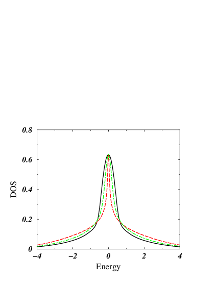
Figure 4: Densities of states for $U=2$, $n=2$ (half-filled case) calculated within the second-order perturbation theory (dot-dashed line), electron-electron TMA (solid line), and electron-hole TMA (dashed line). The one-particle propagators are fully renormalized in the self-consistent calculations ($\Sigma=\Sigma[G]$).

As it is known from the single-band situation, neither of the FLEX-type approximations is able to trace the emergence of satellite Hubbard bands and the metal-insulator transition. The high-energy spectrum is shapeless and broadened due to energy convolutions. This situation changes dramatically if we keep only the topological self-consistence of the one-particle propagators obtained from the IPT, see figure 5. We can see that second order and the electron-electron TMA produces the Hubbard satellite bands in their correct positions. The SOPT scatterings add an additional internal structure to the satellite bands. While the satellite bands gain more weight than they actually have at this interaction strength, the central quasiparticle peak weight is strongly reduced in non-self-consistent or partly self-consistent approximations. Too much quasiparticle weight is transferred to the Hubbard bands.

In the electron-hole scattering channel we get slight changes in the positions of the Hubbard bands, and slight decrease of the quasiparticle width. Even for rather weak interactions $U<1$ one observes nearly total disappearance of the quasiparticle peak when including the electron-hole scattering channel. Due to this unphysical behavior at moderate electron coupling and the instability towards the local state formation we leave the electron-hole scattering channel out from further considerations. There is no way at the FLEX level to improve upon the results from the electron-electron scattering channel. The best we could do is to add contributions from all three distinct channels. But we had to subtract second order contribution to the self-energy which dominates at moderate and intermediate couplings so that we obtain negative density of states at the Fermi energy. The only real improvements can be reached by a new self-consistent coupling of the electron-electron and electron-hole channels of the parquet type. Since we are not yet able to implement parquet-type self-consistence in multiorbital models and have to stay within FLEX, we compare only results of analytical approximations based on second order perturbation theory and electron-electron $T$-matrix against QMC data.

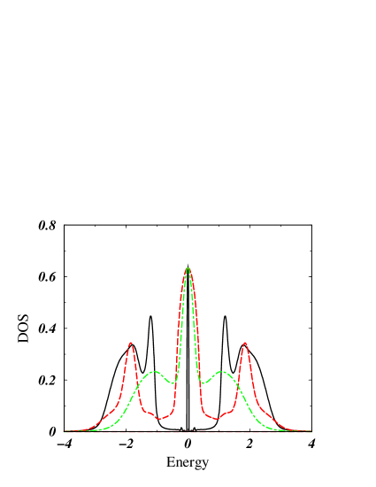
Figure 5: Densities of states for $U=2$, $n=2$ (half-filled case) calculated within the second-order perturbation theory (solid line), electron-electron TMA (dashed line), and electron-hole TMA (dot-dashed line). The one-particle propagators are partially renormalized by using the iterated perturbation method ($\Sigma=\Sigma[\mathcal{G}_{0}]$).

To compare the analytic FLEX results with quantum Monte Carlo simulations, we use both versions of the self-consistency. In figure 6 the density of states at $U=1$ calculated within the electron-electron $T$-matrix approximation is shown along with the one deduced from the QMC. As one can see from the plot, the conserving TMA fits better the quasiparticle peak than the TMA with the IPT bath Green function $\mathcal{G}_{0}$. In addition, the IPT TMA seems to overemphasize the role of the satellite peaks at weak coupling as there are no satellites in the QMC solution for this coupling strength. If we increase the interaction to $U=2$ (see figure 7) and compare the same curves as in the previous plot, we notice that the conserving TMA still very well reproduces the quasiparticle peak, whereas the IPT TMA keeps the tendency to reducing the central peak in favor of the satellites. At this coupling the satellites are formed also in the QMC solution but not as strongly as the IPT TMA predicts. Notice that positions of the satellites reproduced by the IPT solution are rather close to the ones coming from QMC.

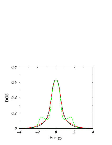
Figure 6: Densities of states for $U=1.0$, $n=2$ (half-filled case) calculated within the electron-electron TMA using the full renormalization of the one-particle propagators (dashed line) and partial renormalization using the IPT (dot-dashed line) compared with the result of quantum Monte Carlo method (solid line).

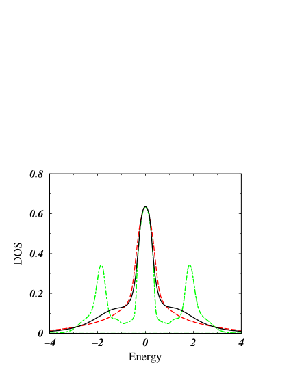
Figure 7: Densities of states for $U=2.0$, $n=2$ (half-filled case) calculated within the electron-electron TMA using the full renormalization of the one-particle propagators (dashed line) and partial renormalization using the IPT (dot-dashed line) compared with the result of quantum Monte Carlo method (solid line).

As a summary of the FLEX for the symmetric case of the multiband Hubbard model we present dependence of the quasiparticle residue, $Z$, on the interaction strength, $U$. It is clear that the closer $Z(U)$ curve for a particular approximation to the QMC data the better the approximation works in reproducing the quasiparticle properties of the system, including the central peak weight and width. In figure 8 we presented the following curves: QMC data are plotted by solid curve with open circle symbols, results of the second order perturbation theory in the cases of fully renormalized one-particle propagators in the self-consistent calculations ($\Sigma=\Sigma[G]$) and partially renormalized by using the iterated perturbation method ($\Sigma=\Sigma[\mathcal{G}_{0}]$) are given by dashed and dot-dashed lines correspondingly. Concentrating on small and intermediate values of interaction, we can see that in the first case of the full renormalization of the propagators the situation is significantly better as the dashed curve goes much closer to the QMC one than the dot-dashed curve. The electron-electron TMA gives even better results than those obtained from SOPT. Both the electron-electron TMA curves, for the case of the full self-consistency ($\Sigma=\Sigma[G]$) plotted by solid line and the partial one ($\Sigma=\Sigma[\mathcal{G}_{0}]$), plotted by dotted line, lay much closer to the QMC data than the SOPT curves (for interactions smaller or equal to $U=2$). From the two electron-electron TMA curves we make a decision in favor of the one obtained using the fully renormalized one-particle propagators in the self-consistency procedure. This result differs from the findings in the case of the one-band Hubbard model, where partially renormalized propagators gave better agreement with Monte Carlo results. Note that the FLEX-type approximations follow the Monte Carlo quasiparticle weight only for weak and moderate interaction strengths, $U\leq 2$. All approximations except for IPT go wrong near and beyond the expected metal-insulator transition.

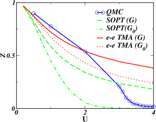
Figure 8: Dependence of the quasiparticle residue $Z$ on Coulomb repulsion $U$ calculated within the electron-electron TMA (solid and dotted with crosses lines) and the second-order perturbation theory (dashed and dot-dashed lines) using the full renormalization of the one-particle propagators and partial renormalization using the IPT correspondingly. QMC results are plotted by solid line with circle symbols.

In figure 9 we study dependence of DOS, calculated by different methods, on orbital degeneracy. We calculated DOS within two- and three-band Hubbard models in the half-filled case using QMC as the tester against two best FLEX approximations which we found, namely, electron-electron TMA with the full self-consistency ($\Sigma=\Sigma[G]$) and the partial one ($\Sigma=\Sigma[\mathcal{G}_{0}]$). One can almost immediately notice the main difference between the QMC and FLEX results. The width of quasiparticle (QP) peak in QMC calculation is slightly increased with the degeneracy. This is expectable as while the degeneracy grows the critical $U$ also increases what brings the curve $Z$ versus $U$ dependence (see figure 8) to go higher for the larger degeneracy at any particular repulsion. As an example the quasiparticle residue against repulsion at $U=2$ for degeneracy $N=6$ will be above the curve in figure  8 corresponding to degeneracy $N=4$. FLEX results show opposite dependence: the QP width decreases with increasing degeneracy. We should also notice that this wrong tendency is stronger for the partial (IPT) self-consistency. The reason for such kind of behavior can lay in a limited set of diagrams treated in FLEX resulting in unsufficient screening for higher degeneracy.

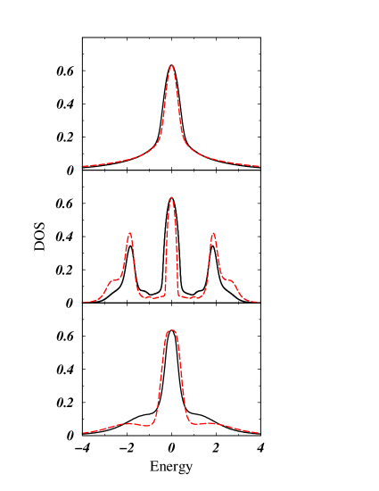
Figure 9: Densities of states for $U=2.0$, $n=2$ in the two-band model (solid lines) and $n=3$ in the three-band model (dashed lines) (both cases correspond to half-filled case) calculated within the electron-electron TMA using the full renormalization of the one-particle propagators (upper panel) and partial renormalization using the IPT (middle panel) compared with the result of quantum Monte Carlo method (lower panel).

The self-consistent FLEX scheme was found to reproduce quite well the central quasiparticle peak for two and three bands at weak and medium interaction strength. It is, however, important to stress that this cannot persist to very large degeneracy. It has been shown [18] that in the exact solution of the DMFT equations for large $N$ the critical $U$ where the Mott transition takes place at zero temperature, scales linearly with $N$. This implies that for fixed $U$ the quasiparticle residue, which has an approximate expression, $Z=1-U/U_{c2}$ increases and eventually approaches unity with increasing orbital degeneracy. This remarkable screening effect in the multiorbital degenerate Hubbard model is not captured by the FLEX approach which displays the opposite trend, as can be seen in figure 10.

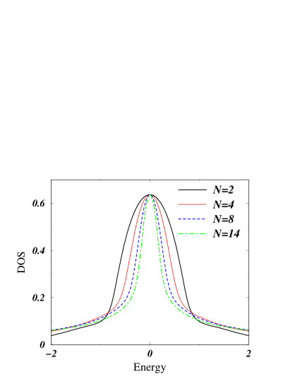
Figure 10: Densities of states for $U=2.0$ ($n$ is kept at the half-filling) calculated within the electron-electron TMA using the full renormalization of the one-particle propagators for different degeneracy (see the legend).

When we move off the electron-hole symmetric case, the situation changes. The quasiparticle peak is no longer so strongly suppressed in the electron-hole scattering channels. Moreover, the conserving TMA starts to develop a satellite peak. Figure 11 demonstrates this trend for $n=0.8$. We perceive almost no difference in the form of the central peak in the two different self-consistent versions of the multiple electron-electron scatterings. The IPT version retains its tendency to overemphasize the width of the satellite peaks and produces an incorrect position of the upper Hubbard band. The conserving TMA shows a shoulder behavior where the QMC displays the hole satellite. The less pronounced electron peak cannot be traced neither in the IPT TMA nor in the conserving TMA.

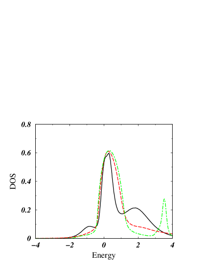
Figure 11: Densities of states for $U=2.0$, $n=0.8$ (partially filled band) calculated within the electron-electron TMA using the full renormalization of the one-particle propagators (dashed line) and partial renormalization using the IPT (dot-dashed line) compared with the result of quantum Monte Carlo method (solid line).

To explore a wider range of parameters away from half-filling we plot the quasiparticle residue dependence on filling in figure 12. With the increment of filling $n$, the scattering rate is increased as number of particles which can scatter a particular electron in the system grows. Therefore it is natural to expect the reduction of quasiparticle residue as the function of $n$ at least for filling $n<1$. As one can see from the plot, the relative positions of the curves are not changed in comparison with figure 8 as well as the conclusion that the electron-electron TMA fits best the QMC data. In addition, one can conclude that for densities $n<1$ both methods (the self-consistent and the non-self-consistent electron-electron TMA work very well describing QMC data, while for $n>1$ we observe a deviation of FLEX from QMC data indicating necessity to take into account other scattering channels. The minima in $Z(n)$ at $n=1$ and $2$ observed in QMC data get even more pronounced with increasing $U$ and indicate the trace of the metal-insulator transition which appears for the two-band Hubbard model at $U\approx 3.5$ as one can see from figure 8. As we mentioned above, the FLEX fails to reproduce the MIT which is also reflected in an almost monotonic decrease of the quasiparticle weight for all densities including interval between $n=1$ and $n=2$.

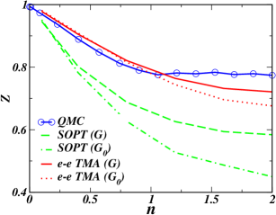
Figure 12: Dependence of the quasiparticle residue $Z$ on filling $n$ for $U=1$ calculated within the electron-electron TMA (solid and dotted with crosses lines) and the second-order perturbation theory (dashed and dot-dashed lines) using the full renormalization of the one-particle propagators and partial renormalization using the IPT correspondingly. QMC results are plotted by solid line with circle symbols.

We mention in passing that the one-band situation is exceptional because the exact evaluation of the one-particle Greens function shows that interaction is not efficiently screened. Therefore, the non-self-consistent version of SOPT theory works well. Furthermore, in the one-band case, the SOPT form combined with the DMFT self-consistency condition produces the correct atomic limit [3], this is not the case in the degenerate situation. In the multiorbital case, the effective interaction is more screened with increasing degeneracy. The self-consistent version of FLEX, attempts to capture this effect, and in fact it does it slightly better than the self-consistent SOPT. The non-self-consistent version of SOPT is worse because it does not screen the interaction at all.

4 Conclusion

In summary, we compared multiband implementation of the FLEX procedure within the framework of the two-band model with semi-elliptic non-interacting DOS against the quantum Monte Carlo method. Obtained results indicate the best agreement with the QMC data is reached for the electron-electron TMA and with fully renormalized one-particle propagators, $\Sigma=\Sigma[G]$. This conclusion is restricted to small energies within the quasiparticle peak and to the region of moderate Coulomb interaction, ($U\leq 2)$. Our finding is somewhat different from that for the one-band Hubbard model, where the best match for the same interaction strengths was found for the one-particle propagators partially renormalized by using the iterated perturbation method ($\Sigma=\Sigma[\mathcal{G}_{0}]$). In the multiband situation for not high band degeneracy and small to intermediate $U$ the self-consistent version describes the quasiparticle features in good agreement with QMC. On the other hand, there is no hint in the self-consistent calculation of an incipient Mott transition, as in the one-band case [19], while the non-self-consistent scheme clearly gives a hint that a Mott transition will take place, albeit at a very small unphysical value of $U$, due to an improper screening of this interaction.

Unsufficient screening due to a limited set of diagrams treated in FLEX results in a quasiparticle weight underestimation with increasing degeneracy in the system. For non-symmetric case, FLEX has tendency to overestimate the QP width and underestimate the Hubbard bands weight given their correct position in the case of conserving TMA. Our results, found for an impurity solver used within the DMFT, have wider range of validity as they are naturally applied to the multiorbital Anderson model as well.

References

- [1] Hohenberg P and Kohn W 1964 Phys. Rev. 136 B864
- [2] Kohn W Rev. Mod. Phys. 1999 71 1253
- [3] Georges A, Kotliar G, Krauth W and Rozenberg M Rev. Mod. Phys. 1996 68 13
- [4] Turek I, Drchal V, Kudrnovský J, Šob M and Weinberger P 1997 Electronic Structure of Disordered Alloys, Surfaces and Interfaces (Boston-London-Dordrecht: Kluwer Academic/Plenum Publishers)
- [5] Kajueter H and Kotliar G 1996 Phys. Rev. Lett. 77 131-134
- [6] Drchal V, Janiš V and Kudrnovský J 1999 in Electron Correlations and Materials Properties edited by A. Gonis et al. (New York: Kluwer Academic/Plenum Publishers) p. 273
- [7] Drchal V, Janiš V and Kudrnovský J 1999 Phys. Rev. B 60 15664
- [8] Bickers N E and Scalapino D J 1989 Ann. Phys. (N.Y.) 193 206
- [9] Abrikosov A A, Gorkov L P and Dzyaloshinski I E 1975 Methods of Quantum Field Theory in Statistical Physics (New York: Dover)
- [10] Kajueter H 1996 Ph.D. thesis (New Brunswick New Jersey: Rutgers University Graduate School)
- [11] Hirsch J E and Fye R M 1986 Phys. Rev. Lett. 56 2521
- [12] Hirsch J E 1983 Phys. Rev. B 28 4059
- [13] Takegahara K 1992 J. Phys. Soc. Jpn. 62 1736
- [14] Drchal V, Janiš V and Kudrnovský J 2003 in Electron Correlations and Materials Properties 2 edited by A. Gonis et al. (New York: Kluwer Academic/Plenum Publishers) p. 341.
- [15] Katsnelson M I and Lichtenstein A I 1999 J. Phys.: Cond. Matt. 11 1037
- [16] Katsnelson M I and Lichtenstein A I 2000 Phys. Rev. B 61 8906
- [17] Kanamori J 1963 Prog. Theo. Phys. 30 275
- [18] Florens S, Georges A, Kotliar G and Parcollet O 2002 Phys. Rev. B 66 205102
- [19] Menge B and Müller-Hartmann E 1991 Z. Phys. B 82 237