Information Super-Diffusion on Structured Networks

Abstract

We study diffusion of information packets on several classes of structured networks. Packets diffuse from a randomly chosen node to a specified destination in the network. As local transport rules we consider random diffusion and an improved local search method. Numerical simulations are performed in the regime of stationary workloads away from the jamming transition. We find that graph topology determines the properties of diffusion in a universal way, which is reflected by power-laws in the transit-time and velocity distributions of packets. With the use of multifractal scaling analysis and arguments of non-extensive statistics we find that these power-laws are compatible with super-diffusive traffic for random diffusion and for improved local search. We are able to quantify the role of network topology on overall transport efficiency. Further, we demonstrate the implications of improved transport rules and discuss the importance of matching (global) topology with (local) transport rules for the optimal function of networks. The presented model should be applicable to a wide range of phenomena ranging from Internet traffic to protein transport along the cytoskeleton in biological cells.

PACS: 89.75.Fb, 89.20.Hh, 05.65.+b, 87.23.Ge

I Introduction

Properties of different types of networks have begun to attract the interest of statistical physicists. The spectrum of network related problems include, among many others, ordinary traffic in a city cartraffic , distribution of nutrients in the vascular system west , distribution of goods and wealth in economies, queuing problems on information networks traffic ; queuing , biochemical- and gene expression pathways genetic_nets . It has been recognized that most natural and man-made networks evolve in time and that their structure emerged as result of microscopic evolution rules SD . In many networks a scale-free linking structure was found SD ; AB which emerges from complex processes of self-organization with specific constraints. Maybe the most prominent example of such a scale-free network is the world-wide Web Web ; BT and the Internet Internet_structure . Transport processes on networks, such as traffic of information packets on the Internet or diffusion of signaling molecules in a biological cell, are physical processes which are closely related to the network geometry. It is likely that biological networks have been optimized in structure by selections in evolution. The vast research on information traffic on technological networks is motivated to optimize network structure for practical reasons such as, e.g., optimum connection strategies and information flow at minimal costs and risk. Technological networks like the Internet or the world-wide Web are relatively easily accessible for empirical research in contrast to e.g. biological networks such as metabolic pathways. A further important motivation for studying networks is to gain theoretical insight in the role of an underlying geometry on the function of a network.

Recent empirical studies on Internet traffic suggest a complex interplay of queuing behavior queuing , temporal correlation in packet streams erramilli ; t1 , and broad distributions of travel times of packets t1 . Moreover, evidence is gathered that both traffic parameters (traffic intensity, buffer sizes, link capacities) and network connectivity play a role in the overall network’s performance. Often two general regimes of traffic are recognized in networks: free flow and jammed traffic. A jamming transition is expected when traffic density exceeds a critical value.

In numerical work recently a model of packet transport was introduced TR which studies simultaneous random walks to specified destinations on scale-free networks. The results suggest that fat-tailed transit-time distributions and temporal correlations may occur for a wide range of values of packet densities as a consequence of network structure TR . Other theoretical models were able to capture essential properties of the jamming transition on simple network geometries, like hierarchical trees Albert_ht and square lattice models Albert_sq ; Sole1 ; Sole2 .

In this work we implement a general numerical model to study packet traffic on several classes of networks with diverse structural characteristics. These include a highly organized cyclic scale-free graph and two types of tree-like graphs. By working in a stationary traffic regime below the jamming transition, our aim is to relate a given network topology to characteristic diffusion parameters such as probability distributions of travel times and packet velocities. Further we want to quantitatively characterize the diffusion on given network topologies within a general framework of non-linear diffusion phenomena.

Quite generally, transport on networks can be seen as a diffusion on a geometry which is not plane- or space filling. Diffusion on such topologies has been a matter of interest over the past decades. Many problems like the diffusion of water particles in a sponge, or crude oil in porous media are phenomenologically well described by the anomalous diffusion equation. Anomalous diffusion is naturally linked to power laws in the corresponding spatio-temporal probability distributions. It has been shown that the probability density which maximizes entropy of a version of a non-extensive entropy definition tsallis88 is an exact solution of the anomalous diffusion equation tsallis96 . It is part of this work to notice the connections between transport on networks and anomalous diffusion and to use the latter to quantify topology-dependence of network performance.

Queuing processes on networks are currently subject of intensive study. Mathematically, being composed of many random processes, network queues are a natural laboratory to study limit stochastic processes. The existence of stable laws in these processes is expected book_spl . However, the connection between the character of the limit process and network structure remains an open theoretical problem. Having numerically determined large series of transit-times of packets we also attempt to recognize their convergence to a stable law and explore the consequences of it on specific network topologies.

In Section II we specify the model of network diffusion and describe details of network structures and the implementation of diffusion rules. We determine conditions of the stationary (un-jammed) regime for all network topologies. In Section III the results for transit-times distributions are presented in the stationary regime. We show results for the limit of infinitely low packet density on networks and discuss the statistical regularity of transit-timeseries. Section IV motivates the use of anomalous diffusion methods in network transport and contains the results of the velocity distributions on different networks. In Section V we study temporal correlations of workload timeseries and in Section VI we summarize and discuss the results.

II Model of Non-linear Diffusion on Networks

A fundamental problem in non-linear diffusion is to understand how the topological structure or the sparseness of space affects the dynamics that it supports. Transport on a complex network with local navigation rules is a prototype for diffusion on a sparse structure. Further reasons for non-linear terms in diffusion equations can be related to the diffusion process itself, i.e., to the specific way of local navigation between individual nodes and queuing properties. In this work we introduce a numerical model in which we can control both, graph topology and microscopic diffusion details (transport rules). We consider graphs with link structure that emerges from controlled microscopic linking rules, from which the graphs are grown. We grow three different types of networks (described in detail below) consisting of an equal number of nodes ($N=1000$) and links ($E=1000$) but having different linking patterns. After specifying the diffusion rules we monitor the simultaneous transport of packets on these graphs, and analyze local and statistical properties of the resulting traffic. A packet (particle) carries information from the node where it is created to an in-advance specified node (address) on the network. These can be, for instance, a piece of information transported on the Internet or a protein in a biological cell.

II.1 Types of networks

To determine how the structure of links in the network influences diffusion, we study three topologies with emergent link structures. Their main structural characteristics are the following: (i) Scale-free directed graph with closed cycles (cyclic Web graph, WG); (ii) Scale-free graph with no closed cycles (scale-free tree, SF); and (iii) Absence of a scale-free structure and absence of closed cycles (randomly grown tree, RG).

For all cases we stop growth of the graph when $N=E=1000$ nodes and links have been added. All the graphs that we consider have the same number of nodes and links, they differ in the adjacency matrix. After growing the network, the corresponding adjacency matrix is not changed during the diffusion processes.

II.1.1 The Web graph (WG) as a scale-free cyclic graph

We first consider the scale-free cyclic graph (WG) shown in Fig. 1a. Such a graph is grown by adjusting a single free parameter governing microscopic linking rules proposed in BT . These rules have been suggested as an evolution model of the world-wide Web. The minimal set of rules consists of: growth by adding of a new node at each time step and attachment (with probability $\tilde{\alpha}$) of the new node to a pre-existing node, or rewiring (with probability $1-\tilde{\alpha}$) of a pre-existing node. Each link is oriented originating from a node, $n$, as an out-going link, and pointing to another node, $k$, where it is seen as in-coming link. In the model BT ; BT_ccp02 both the target node $k$ and and the origin $n$ of a link are selected by shifted preferential probabilities given by

$$p_{in}=(M\alpha+q_{in}(k,t))/(1+\alpha)Mt\ ;\ p_{out}=(M\alpha+q_{out}(n,t))/(1+\alpha)Mt\ ,$$ (1)

which depend on the number of respective in-coming links $q_{in}(k,t)$, and out-going links $q_{out}(n,t)$ at current time $t$. The shift parameter $\alpha$ is the initial probability, where $q_{in}(k,0)=q_{out}(n,0)=0$. $M$ is the average number of links added per time step. As shown in BT ; BT_ccp02 the biased attachment and rewiring in the growth rules lead to a scale-free organization of both in- and in out-links with the local connectivity at node $s$ at time $t$ building up in time with a power-law

$$q_{in}(s,t)=A_{1}\left[\left(t/s\right)^{\gamma_{in}}-B_{1}\right]\ ;q_{out}(s,t)=A_{2}\left[\left(t/s\right)^{\gamma_{out}}-B_{2}\right]$$ (2)

where the scaling exponents are $\gamma_{in}=1/(1+\alpha)$, and $\gamma_{out}=(1-{\tilde{\alpha}})/(1+\alpha)$. The power-law growth of the local connectivity in Eq. (2) ensures an emergent scale-free structure of the graph after long evolution time. The global graph structure at $t\to\infty$ is thus characterized by the power-law distributions of links BT ; BT_ccp02 ; SD , $P(q_{in})\sim q_{in}^{-\tau_{in}}$ and $P(q_{out})\sim q_{out}^{-\tau_{out}}$ with $\tau_{in}=1+\gamma_{in}^{-1}$ and $\tau_{out}=1+\gamma_{out}^{-1}$. Here we use the original one-parameter model BT with $\alpha=\tilde{\alpha}=1/4$ and $M=1$. Apart from the scale-free organization of in- and out-links, the emergent graph structure is characterized by the occurrence of closed cycles of directed links and a single giant connected component. Two types of hubs (nodes with a large in-link and nodes with a large out-link connectivity) appear together with a substantial degree of correlations between local in- and out-connectivity BT_ccp03 . Recent analysis of empirical data on the structure of the Internet Internet_structure reveal similar topological properties on the level of routers. This type of graph topology has also importance in biological scale-free networks (metabolic networks) cell ; metabolic_nets , where the presence of closed cycles enables feedback regulation. As a further example we mention gene co-regulation networks genetic_nets . After a gene is expressed its product molecules (mRNA or proteins) are in part addressed to specific genes in the network where they bind and regulate the expression of the other genes. Another biological network which shares some characteristics of the WG is the cell crawling network, where cells move along dynamic paths traced by previous cells mombach ; Stefan .

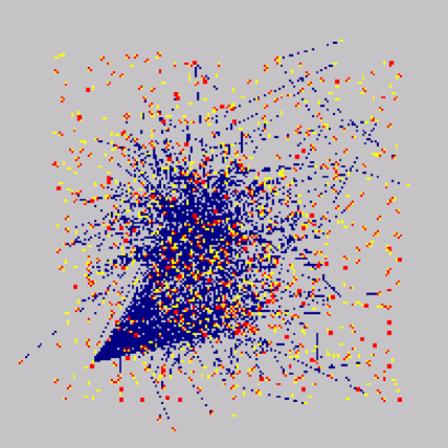
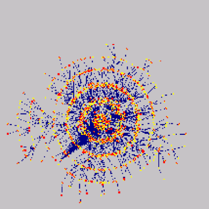
$(a)$	$(b)$

Figure 1: (a) Web graph (WG) and (b) scale-free tree graph (SF) composed of the same number of nodes and links, $N=E=1000$. The graphs are grown from the microscopic rules described in the text and in Ref. BT . The first hub node is pulled towards the lower left corner for better vision. In the WG an additional hub is visible in the central part of the figure. Typical layers of nodes linked to preceding layers are seen as circular arrangements in the SF, which are absent in the WG. Disconnected nodes occurring in the WG have a finite probability to increase both in- and out-link connectivity if the graph continues to grow, while in the SF the out-link connectivity of the nodes remains fixed.

II.1.2 The scale-free tree graph (SF)

To grow the scale-free tree graph (SF) we use the shifted preference rule with $p_{in}$ given in Eq. (1), but we suppress rewiring of links by fixing the parameter $\tilde{\alpha}=1$, and set the parameter $M=1$. Therefore each added node connects immediately to a pre-existing one, which is selected with a probability $p_{in}$ in Eq. (1), and the link remains fixed in the subsequent evolution of the graph. For a characteristic look of such a graph, see Fig. 1b. For better comparison, for the SF graph we chose the shift parameter $\alpha=1/4$, so that the in-link connectivity is described by the same power $\gamma_{in}$ as the WG in Eq. (2). However, the out-links remain evenly distributed, i.e., one link per node, hence making the overall graph structure less organized compared to the WG. In particular, only a hub with large in-link connectivity can occur. When the number of links added per step $M$ exceeds one the tree structure is lost and the graph can have multiple paths from one node to another. These may be considered as cycles if the directedness of the links is disregarded, in contrast to the WG where closed cycles along strictly directed links occur even for $M=1$. Another structural difference of the SF and the WG is the absence of correlations between local in- and out-connectivities in the SF. The SF (with general $M$) is most often called scale-free network in the literature AB ; SD ; TR .

II.1.3 The randomly grown tree graph (RG)

The randomly grown tree graph is grown in the same way as the SF tree except that the target node for each link is selected randomly among all the pre-existing nodes. At time $t$ the probability to link to a selected node is $p_{in}(t)=t^{-1}$. This linking rule leads to a local connectivity increase which is logarithmic in time rather than a scale-free law. The out-link connectivity remains fixed with one link per node. In the present context the RG is the least organized or structured graph.

II.2 Diffusion rules on the network

Given the graph structure in form of the adjacency matrix, diffusion of packets is defined by specifying the following steps (see also TR ; BT_ccp03 ):

• Creation and assignment: A packet is created with rate $R$ (posting rate) at a randomly selected node and it is assigned a destination address on the graph.

• Diffusion rules: Before reaching its destination a packet passes from a node to one of its neighbors, being directed by local search algorithms (diffusion rules). For the selection of a neighbor we implement two algorithms:

  (1) Random diffusion (RD): The packet is passed from a given node to one of its neighbors with equal probability;

  (2) Cyclic Search (CS): The node performs a next-to-nearest-neighbor (nnn) search in its neighborhood, looking if the destination address of the packet is within nnn distance. If it gets a signal that the address was found within a nnn surrounding, the node passes the packet to that neighbor. If the address is not within nnn it uses the random diffusion rule (1).

• Queuing strategy: When more than one packet is sitting on a node a queue is formed and a queuing discipline needs to be specified. Here we mainly focus on the first-in-first-out (FIFO) queue, but also study the last-in-first-out (LIFO) strategy. A packet can only be processed if the current queue size at a selected neighbor node is bellow some maximal allowed buffer size $H$, otherwise it waits for the next occasion to be processed. For simplicity, we treat diffusion along out-links and against in-links with equal probability. The model allows for various other possibilities.

• Removal: When a packet reaches its destination it will be removed from the network.

To implement these steps one first defines a time step by one parallel update of the entire network. At each time step we create packets with rate $R$ and assign them their destination addresses. In order to avoid sending packets to a disconnected part of the graph we specify the list of nodes belonging to the giant component of the WG. The pairs of nodes (origin and destination) is selected randomly from that list. The same list is used for all three graph types. At each time step we also keep track of the packets’ current positions, and their positions within a queue at given node. For temporal traffic statistics we label a certain number of packets so that we monitor their creation time, the time that a packet spent at a current node, and the total elapsed time before being delivered to its destination. In our setup we label 2000 packets. The length of a particular simulation for a given network and search algorithm depends on the posting rate $R$. We keep updating the system until the pre-fixed number of labeled packets have been created and arrived at their destinations. Results are averaged over many network realizations. We typically use 100 sample networks for each simulation. Details of the numerical implementation of the code can be found in Ref. BT_ccp03 .

II.3 Stationary Flow and Slow Driving

To be able to entirely focus on the network structure and not to be troubled with queuing effects at individual nodes, we assume a large buffer $H=1000$ at each node and apply a posting rate $R$ such that the number of packets present in the system fluctuates around a finite value considerably below the maximal queue size $H$. An example of stationary flow is shown in lower two panels in Fig. 2.

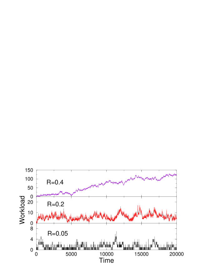
Figure 2: Number of packets in the WG network as a function of time (workload) for the advanced search algorithm (CS) and different posting rates $R=0.05$, $R=R^{\star}=0.2$, and $R=0.4$.

Stationarity is established by the balance of the network’s input rate $R$ and its output rate $\rho$, i.e., the number of delivered packets per time step. The output rate $\rho$ is a parameter which depends on the network topology and the diffusion rules. The number $n(t)$ of packets in the system at current time $t$ and is called workload. When the posting rate exceeds a certain limit, the workload $n(t)$ shows a persistent increase, which is related to the occurrence of jamming (full buffers) in the network. In fact for several networks there exists a phase transition from a free-flow phase to a jammed phase Sole1 . Here we do not discuss the onset of jamming, our aim is to study properties of traffic on different networks in stationary flow below the jamming transition. Values of the posting rate $R$ for which a stationary flow is sustainable appear to be crucially dependent both on network topology and search algorithms. To be able to compare the efficiency of a given network, we select to work with a posting rate $R^{\star}$, for which the workload fluctuates within same limits when different search algorithms are used. As a rule, when the rate is increased above $R^{\star}$, jamming will first occur in the case of less efficient search. The values for $R^{\star}$ for two search algorithms in the three types of graphs are summarized in Table 1.

	$R^{\star}$ (CS)	$R^{\star}$ (RD)	Ratio CS:RD
WG	$2\times 10^{-1}$	$5\times 10^{-3}$	$40$
SF	$5\times 10^{-3}$	$1\times 10^{-3}$	$5$
RG	$1\times 10^{-2}$	$5\times 10^{-3}$	$2$

Table 1: Values of posting rates $R^{\star}$ for the search algorithms CS and RD and different graphs. The ratio CS:RD shows the efficiency increase of the CS relative to RD for given graph topology.

The improvement of efficiency of the advanced local nnn-search relative to random diffusion is shown for the different topologies in the column ”Ratio CS:RD”. In the stationary regime within a given time interval the cyclic WG manages to process 40 times more packets by using CS than when using RD. The same search algorithm is doing five times better on the SF tree, and only a factor two on the RG.

As a limiting case where queuing is completely absent we define the zero posting rate limit, $R\to 0$, where a new packet is created only after the previous one is delivered at its destination. This means that there is only one packet in the system at any time. Although this limit is not accessible in real network traffic, it is mathematically interesting because the absence of queuing allows to single out topology effects on non-linear diffusion.

III Transit times on different graph topologies

Transit time $T$ is the time a packet spends on the network from posting until arrival at its destination. It is primarily related to the number of jumps the packet performs on the graph which is crucially dependent on the topology and the search algorithm. For a finite posting rate $R>0$ the effects of queuing also contribute to the transit-time. For a given packet the transit-time is determined as

$$T_{k}=\sum_{i=1}^{k}t_{w}(i)\quad,$$ (3)

where index $i$ denotes nodes along the actual path of the packet, and $t_{w}(i)$ is the packet’s waiting-time at node $i$ along the path. $k$ is the total length of the path taken by the packet. We determine the probability distribution of transit-times, $P(T)$, in the stationary flow regime. $P(T)$ incorporates two effects which are crucial for the diffusion on networks: the graph topology and waiting-times.

III.1 The $R\to 0$ limit

Consider the $R\to 0$ limit, where queuing is absent, rendering all waiting-times $t_{w}(i)=1$. Hence the transit-time of a packet is given by the number of jumps before reaching its destination. In this limit transit-time probes network topology and efficiency of the applied search on that topology. In Fig. 3 (left column) we show the transit-time distribution for the three network topologies WG, SF, and RG, and for the two search algorithms RD and CS. The results suggest that topology strongly matters when the advanced local search CS is applied, resulting in drastically shorter transit-times, especially for the WG graph. Differences are also seen between the SF and RG tree graphs. For RD differences between the three network topologies become less pronounced.

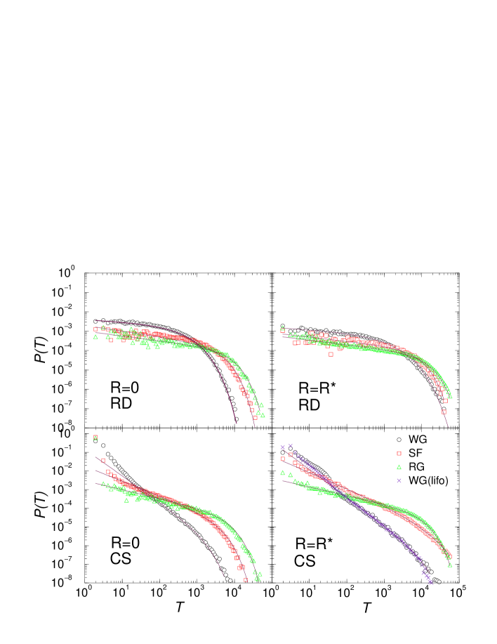
Figure 3: Transit times distribution $P(T)$ for no queuing $R\to 0$ (left column), and stationary flow at respective rate $R=R^{\star}$ (right column) for the three graph topologies. Lower panels show results for the CS algorithm, upper panels for the random diffusion (RD). The distributions are normalized by the total number of arrived marked packets ($2\times 10^{5}$ packets) and are log binned. Solid lines are fits to Eq. (4). Corresponding parameters are given in Table 2.

A prominent feature of the transit-time distribution is the power-law behavior before a cut-off. This is most apparent for CS. The distributions are fitted to the following expression

$$P(T)=A\,T^{-\tau_{T}}\exp{\left[-\left(\frac{T}{T_{0}}\right)^{\sigma}\right]}\quad,$$ (4)

to account for the power-law and for finite size cut-offs. Results are gathered in Table 2. For CS the scaling exponents $\tau_{T}$ vary considerably with network topology from $\tau_{T}\approx 1.5$ for the WG, to $\tau_{T}\approx 0.5$ for the RG. For RD the cut-off time $T_{0}$ increases, in agreement with lower transport efficiency. A small slope $\tau_{T}$ close to $0.25$ was found for both tree networks and almost no power law in the WG. The stretching in the exponential cut-offs is absent in most of the fits, however, for CS on the WG fits improve with a $\sigma=0.6-0.7$.

	random diffusion (RD)						advanced nnn-search (CS)
	$R=0$			$R=R^{*}$			$R=0$			$R=R^{*}$
Measure	RG	SF	WG	RG	SF	WG	RG	SF	WG	RG	SF	WG
$A$	0.001	0.002	0.004	0.0006	0.008	0.003	0.003	0.018	0.12	0.004	0.06	0.38
$\tau_{T}$	0.25	0.30	0.12	0.24	0.22	0.12	0.48	0.80	1.42	0.46	0.86	1.5
$T_{0}$	7000	3900	360	12000	7000	1000	6000	3600	1500	10000	10000	10000
$\sigma$	1	1	0.7	1	1	0.6	1	1	1	1	0.6	1
$q$	1.49	1.38	1.51	1.53	1.46	1.49	1.42	1.81	-	1.64	1.87	-
$\beta$	-	-	-	1.99	2.00	1.98	-	-	-	1.99	1.85	1.35
$\alpha$	-	-	-	0.49	0.49	0.45	-	-	-	0.47	0.39	0.21

Table 2: Fit parameters for the fit of transit-time distributions $P(T)$, as defined in Eq. (4). Also shown are the values for non-extensivity parameter $q$ defined in Eq. (10) and the scaling exponents for the power-spectrum $\beta$ and the profile fluctuations $\alpha$, of workload timeseries on different graphs.

III.2 The $R=R^{\star}$ case

Measurable effects of queuing are expected in the stationary flow at $R=R^{\star}$ on different networks. We monitor waiting-times of labeled packets in detail. On a given graph the statistics of waiting-times is sensitive both to the posting rate $R$ and the search algorithm. In stationary flow long queues are strongly suppressed and waiting-times are generally short in the FIFO queuing. The distribution of waiting-times decays rapidly with $t_{w}$. (The study of long queues at large posting rates $R>R^{\star}$ is left out of this paper.) As a consequence of waiting-times $t_{w}(i)>1$ in Eq. (3) in stationary flow we find that the cut-offs in the distribution of transit-times increase, suggesting a delay in transport. However, the slopes of the transit-time distributions remain roughly the same as in the $R\to 0$ limit. Results are shown in Fig. 3 (right column), both for CS and RD. Fit parameters to Eq. (4) are collected in Table 2 and suggest a persistence of power-laws. It is found that for the WG with CS the queuing discipline only affects the transit-time distribution at short times, whereas the asymptotic power-law behavior persists with a unique exponent. We include the result for the LIFO queuing discipline on the WG for comparison, shown on lower right panel in Fig. 3. As before, the differences between the graph topologies narrow up in the case of random diffusion (see upper right panel in Fig. 3).

The deviation from the power-law at low transit-times for CS on the WG and the SF graphs (see Fig. 3) is a direct consequence of the presence of hub nodes in these graphs. When both the origin and destination node of a packet are in the vicinity of a hub, e.g., up to a three-step separation, a direct path between them is immediately found by CS. The frequency of such an event is directly proportional to the number of hubs in the graph and to the number of nodes linked to these hubs. The excess of the fast transport is reduced at finite posting rate because of queuing at the hub nodes.

III.3 Statistical regularity and graph structure

As seen in Fig. 3 for CS transit-time distributions differ markedly on graphs with different structure. This means that CS makes use of the underlying graph topology to accelerate transport, which leads to the power-law dependences with strictly larger scaling exponents. The power-law behavior of the distributions (apart from a cut-off) ensures that if a stable limit stochastic process exists, it can be related to the graph structure. Here we attempt to characterize the statistical regularity of such a process on the WG.

The transit-time $T_{k}$ for each packet is a partial sum given in Eq. (3). The set of all transit-times $\{T_{k}\}$ is a set of stochastic variables both because of the randomness of path length $k$ (related to topology and search algorithm) and because of the random increments (queuing times) along that path. They both depend on the simulation time, i.e., when and where a packet has been sent, and on the posting rate. We now consider the limit $R\to 0$ (no queuing), where stochasticity arises from topology and search only. Since the distribution of transit-times is a power-law, in theory Prohorov_book ; book_spl all transit-times from the set $\{T_{k}\}$ can be driven from the same probability function (stable law) $G(X)$ by rescaling the argument, i.e., $P(T_{k}<X)=G(c_{k}X-a_{k})$. Here $c_{k}$ is a space-scaling factor, $a_{k}$ the average value and $G(X)$ is the class of stationary distributions. Then the distribution function of the rescaled partial sum converges to the same stable law $G(X)$, i.e.,

$$G\left(k^{-1/\mu}T_{k}-a_{k}\right)\Longrightarrow G(X)\quad.$$ (5)

When $c_{k}=k^{-1/\mu}$ and $0<\mu\leq 2$ it is known that the cumulative probability density function (pdf) which describes the stable law is given by $P(X>T)\sim T^{-\mu}$ book_spl . In the special case for $\mu=1/2$ the stable law is described by Lévy pdf, (see Prohorov_book ; book_spl for details).

The observed scaling exponent $\tau_{T}$ close to 3/2 for the $P(T)$ at large transit-times in the WG with CS, suggests a stable law with $\mu\equiv\tau_{T}-1\approx 1/2$. One may speculate about the kind of limit process which is at the origin of the observed statistical regularity. A Lévy pdf could be certainly understood when associated with a random walk in which long jumps are allowed, or in terms of the relation of the time of the $n$th return of a centered random walk to the origin Prohorov_book , which could be naturally related to cycles in a graph.

As an immediate consequence of the self-similarity expressed in Eq. (5) one could expect the transit-time distribution to scale with path length $k$. To study this we vary the size of graph $N$. As stated in Section II, the pairs of nodes that we consider belong to the giant component of the graph. Since the giant component in the WG scales linearly with the graph size $N$, we expect that the longest path (and thus the transit-time) will scale with $N$. Simulations using different network sizes $N$ show that this is in fact the case as shown in Fig. 4.

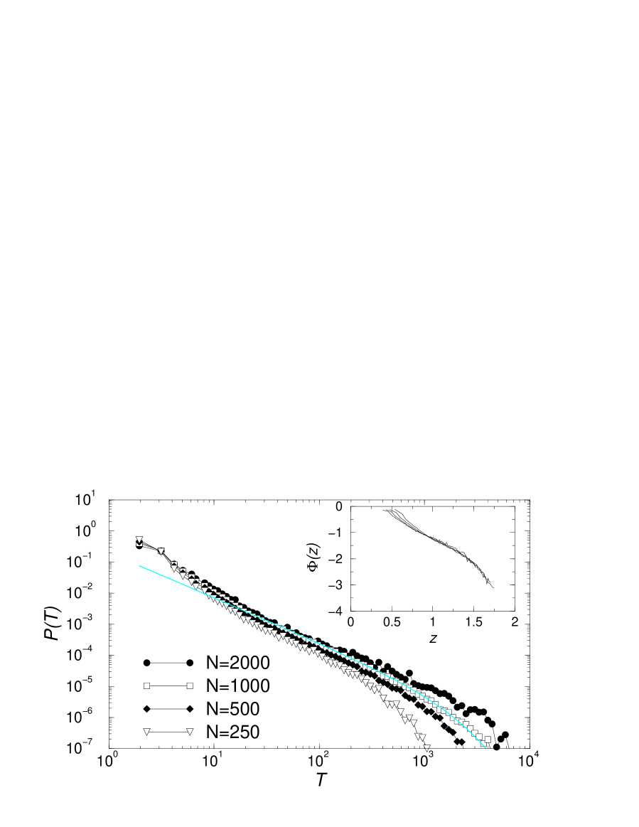
Figure 4: Transit time distribution $P(T,N)$ vs. $T$ for CS on the WG in the $R\to 0$ limit for different network sizes $N$. Inset: Spectrum of dynamic exponents $\Phi(z)$ defined in Eq. (6) with $T_{0}=0.1$ and $N_{0}=1$.

An attempted scaling fit with a unique fractal dimension (dynamic exponent) $z$ according to $P(T,N)=N^{-\tau_{t}z}{\cal{R}}(T/N^{z})$ does not lead to a satisfactory scaling collapse and the scaling function ${\cal{R}}(T/N^{z})$ can not be determined. We try a multifractal scaling fit instead:

$$P(T,N)=\left(\frac{N}{N_{0}}\right)^{\Phi(z)}\quad;\quad z=\frac{\log(T/T_{0})}{\log(N/N_{0})}\quad.$$ (6)

The collapse is found when the scaling parameters $T_{0}$ and $N_{0}$ are suitably selected. The resulting spectral function $\Phi(z)$ (spectrum of dynamic exponents) is shown in the inset to Fig. 4. The range of the spectrum, $0.5\leq z\leq 1.75$, implies that the associated processes on the WG are super-diffusive ($z<2$) with parts of the spectrum in the ballistic region ($z\leq 1$). This can be understood as follows: As the number of nodes in the graph increases the hub nodes become richer in terms of connectivity. Therefore, the probability of a three-link separation between selected pairs of nodes around the hub increases. Transport between such nodes is direct and not diffusive anymore. This fast transport dominates the lower part of the spectrum $\Phi(z)$ in large graphs.

In the tree networks with CS and in all three graphs with RD the scaling exponents (Fig. 3) are found in the range $\tau_{T}\lesssim 1$. These exponents would lead to values $\mu\lesssim 0$, which can not be related to true self-similar limit process implied by Eq. (5). However, the tree network transit-time distributions (Fig. 3) also imply statistical regularity with non-Gaussian pdf. The super-diffusive nature of traffic in these cases can be discussed more conveniently by considering the velocity distributions associated with transit-times on these graphs.

IV Velocity distributions and $q$-statistics

We start with a short summary of the concept of non-extensive entropy, which offers an analytical way to solve a certain class of non-linear diffusion equations. In general, modeling non-linear anomalous diffusion processes involves non-linearities in the associated Fokker-Planck like equations

$$\frac{\partial}{\partial t}p({x},t)=-\frac{\partial}{\partial x}\left(F\left[p\right(x,t)]p(x,t)\right)+\frac{1}{2}\frac{\partial^{2}}{\partial x^{2}}\left(D\left[p\right(x,t)]p(x,t)\right)\quad.$$ (7)

In the following we neglect the flow-term for simplicity $F[p]=0$. To incorporate the idea of anomalous diffusion, the functional dependence of the diffusion parameter in the form $D[p]p=p^{\nu}$ is considered. With this choice Eq. (7) can be solved using the non-extensive entropy approach tsallis88 ; tsallis98 , where classical entropy definition $S=-\int p(u)\ln p(u)du$ is modified to

$$S_{q}=\frac{1-\int p(u)^{q}du}{q-1}\quad.$$ (8)

By maximizing $S_{q}$ while keeping energy fixed it can be shown that the resulting $p(u)$, i.e.

$$p_{q}(x,t)=\frac{\left[1-\beta(t)(1-q)[x-\langle x\rangle(t)]^{2}\right]^{\frac{1}{1-q}}}{Z_{q}(t)}$$ (9)

also solves Eq. (7) without the flow-term tsallis96 ; bologna00 . Here $Z_{q}(t)$ is the generalized $q$-partition function. The relation of the Tsallis entropy factor $q$, and $\nu$ in Eq. (7) is given by $q=2-\nu$ tsallis96 . Note, that this distribution is a power law, and only in the limit $q\longrightarrow 1$ the classical Gaussian $p_{1}(x,t)=\frac{\exp^{-\beta(t)\left[x-\langle x\rangle(t)\right]^{2}}}{Z_{1}(t)}$ is recovered. It can be shown that the corresponding velocity distribution of the associated particles is given by silva98 ,

$$p(v)=B_{q}\left[1-(1-q)\frac{v^{2}}{v_{0}^{2}}\right]^{\frac{1}{1-q}}\ ,$$ (10)

which reduces to the usual Maxwell-Boltzmann result $p(v)=\left(\frac{m}{2\pi kT}\right)^{\frac{3}{2}}\exp^{-\frac{\beta mv^{2}}{2}}$ again in the limit $q\longrightarrow 1$. Here $v_{0}^{-2}\equiv\frac{\beta m}{2}$ can be seen as an inverse mobility factor, meaning that large values of $\frac{\beta m}{2}$ are associated with small average particle velocities. If diffusion on networks is in fact describable as anomalous diffusion governed by a Fokker-Planck equation like Eq. (7) with the special choice of $D\left[p\right]$, the velocity distribution function should follow the general form given in Eq. (10).

IV.1 Defining velocity on networks

On the networks discussed in this paper we have not selected a particular length scale. Moreover, the packets/particles which are sent along the links of the network do not have a particular velocity. In case a packet is not trapped at a node it moves at a rate of one link per one time step. As discussed above, a sensible measure which captures the performance of a network with given topology and search algorithm is the transit-time $T$. Finite transit-times are governed by two effects: (1) The minimum distance of a given pair in terms of the number of links between them, and the deviation of the actual path from the minimum separation; (2) the waiting-times $t_{w}(i)$ at node $i$ along the path taken by the packet.

We consider the minimum distance $d$ between pairs of nodes picked at random on a given graph, which serves as a “linear” scale of a graph. The velocity of a packet transported between a given pair can be defined as the ratio $v=d/T$. The distribution of distance over random pairs carries information about graph topology.

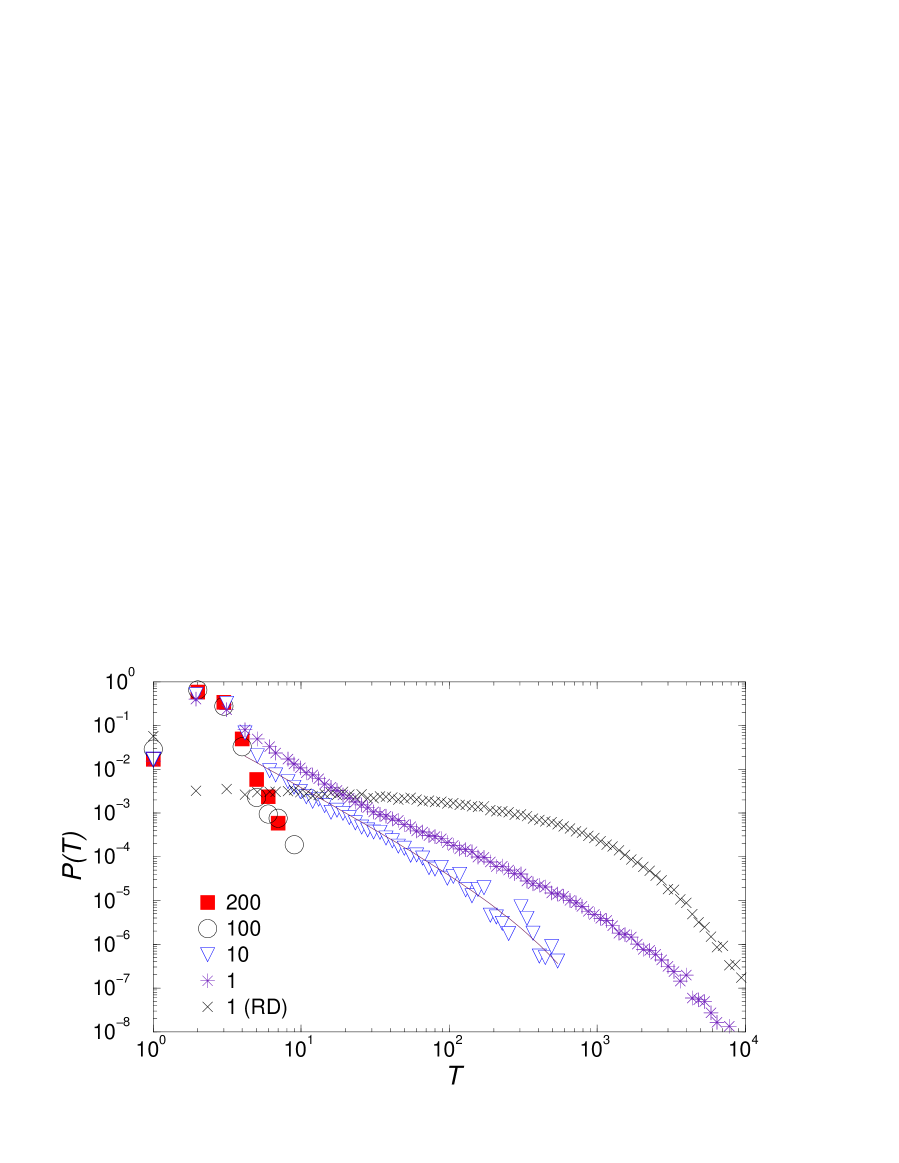
Figure 5: Probability distribution of transit-times $T$ corresponding to shortest separation of pairs in the WG (full squares). Different curves are for the shortest transit-times of 200 (squares), 100 (circles), 10 (triangles) and 1 (*) identically sent packets between the same pair of nodes in the $R\to 0$ limit for CS rule. The case for a single copy sent with RD search is also shown as (X).

Note, that in the $R\to 0$ limit the distribution of minimum path lengths corresponds one-to-one to transit-times of packets if a global optimal navigation is applied. Here we determine the distribution of shortest separations statistically, i.e., as the stable statistics with a large number of trials. For the WG this is a narrow distribution sharply peaked at an average distance $\bar{d}\geq 1$ (Fig. 5). The minimum path is limited by the diameter $\bar{D}$ of the graph $d\leq\bar{D}\propto\log(N)$, which is very small in the structured graphs. Therefore, as a good measure of velocity of packets on the graph we may take $v\sim 1/T$, where $T$ is the actual transit-time of a packet.

The probability distribution of the velocity of traffic at each graph can be either computed directly in the simulations or derived from the transit-time distributions. The situation in both approaches is qualitatively the same. We get somewhat smoother curves for the derived distributions. By noting $p(v)dv=P(T)dT$ we straight forwardly transform

$$p(v)=P(T)\left|\frac{dv}{dT}\right|^{-1}=P(1/v)v^{-2}\quad.$$ (11)

Since the velocity on a graph is by our definition a ratio of stochastic variables, one could expect the probability density function of the form (apart from the finite size cut-offs)

$$p(v)=\frac{\sigma}{\pi(\sigma^{2}+v^{2})^{y}}\quad$$ (12)

where $y\neq 1$ measures deviation from the standard Cauchy pdf. The case $y=1$ corresponds to the pdf of the ratio of two IID variables. In Fig. 6 we show the velocity distributions obtained from the transit-times of Fig. 3 for different graph types. For RD the slope of the velocity distributions on all three graph structures is $\tau_{v}\lesssim-2$. The deviations from $y=1$ are clearly linked to the network topology when CS is used. We suggest to use these deviations as a measure of correlation for a given search algorithm with topology.

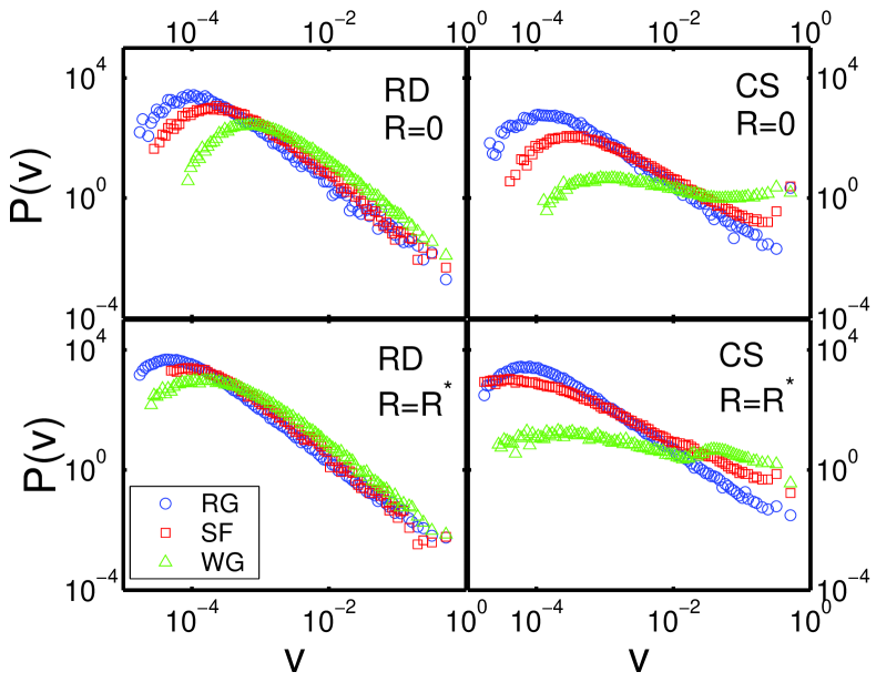
Figure 6: Velocity distributions $p(v)$ for the three networks, for $R\to 0$ (top row), and $R=R^{*}$ (bottom). RD is shown in the left column, CS in the right.

As a generic feature, $p(v)$ has power law tails which extend over several decades. For RD these tails extend to the very end for all networks, while for CS the WG shows a peculiar behavior: For high velocities the probability density moves up again. This is in agreement with increased probability of fast transport in the close vicinity of the hubs, as discussed in Section III.

The distribution $p(v)$ in Eq. (11) for various networks for different posting rates and search algorithms can be compared to the form of Eq. (10). From fits to this curve the value of $q$ can be estimated. Technically, this was done by linear fits to the so-called $q$-logarithm, $q\_\log p(v)=\left[1-p(v)^{1-q}\right]/(q-1)$. For the appropriate value of $q$ this expression becomes a linear function of $v$. $q$ was obtained by finding the minimum of the least square errors of linear fits to $q\_\log p(v)$ as a function of $q$. Results are gathered in Table 2.

Values of $q>1$ are characteristic for the super-diffusive nature of the transport on these graphs tsallis96 . The velocity distribution in the WG in combination with CS has a much lower power exponent which would imply un-physically large $q\gg 2$. This is in agreement with the multifractality of transit-times on the WG, discussed in the previous section. A single value of $q$ probably can not properly describe the character of the process which has the spectrum of the dynamic exponents $\Phi(z)$ shown in Fig. 4.

Note, that the velocity pdf in Eq. (12) is equivalent to the general form in Eq. (10), when parameters are identified as $y\equiv 1/(q-1)$, $\beta m/2\equiv 1/\sigma^{2}(q-1)$, and $B_{q}\equiv\sigma^{(q-3)/(q-1)}/\pi.$ The non-extensivity parameter $q$ in the anomalous diffusion on networks can be directly related to the network structure and correlation between search and topology, indicated by $y\neq 1$.

V Workload timeseries

Another source of information is the workload timeseries $n(t)$ where we look for non-trivial correlations (Fig. 2). Self-similarity of the process and related persistence in a timeseries $X_{t}$ can be characterized by the temporal correlation function of its increment process $I_{t}=X_{t+1}-X_{t}$,

$$C(\tau)=\langle I_{t}I_{t+\tau}\rangle=\frac{1}{N-\tau}\sum_{t=1}^{N-\tau}I_{t}I_{t+\tau}\quad.$$ (13)

For no persistence, i.e., a temporally uncorrelated $I_{t}$ process, $C(\tau)=0$ for $\tau\leq 0$. For persistence up to $\tau_{\rm pers}$ timesteps $C(\tau)$ is positive below $\tau_{\rm pers}$, and vanishes above. Reliable direct computation of $C(\tau)$ is known to be problematic, due to noise, possible non-stationarities or trends and the finiteness of the timeseries thurner97 . We therefore adopt a standard way of proceeding bunde98 , and start from the original timeseries $X_{t}$, interpreting it as the position of a random walker. $X_{t}$ is sometimes called a profile. It is known that for a power-law decay in the correlator

$$C(\tau)\sim\tau^{-\gamma},\quad 0<\gamma<1\quad,$$ (14)

the statistics (standard deviations) of the profile-fluctuations, defined by

$$F(\tau)=\langle(X_{t+\tau}-X_{t})^{2}\rangle_{t}^{\frac{1}{2}}\quad,$$ (15)

also scale according to

$$F(\tau)\sim\tau^{\alpha},\quad\alpha=1-\gamma/2\quad.$$ (16)

There are several possibilities to define $F(\tau)$, which lead to the same (or one-to-one related) scaling behavior. This can be used to eliminate the influence of linear trends in the data. Frequently used definitions are ”detrended” fluctuation analysis, or statistics based on wavelet analysis arneodo95 ; thurner98 . These methods are superior to the direct analysis of the power-spectra since non-stationarities in the data are known to influence the quality of scaling exponents. However, the power-spectrum density, where squared Fourier transforms $S(f)$ of the data are considered, has the advantage of a straight forward interpretation: It directly gives the energy distribution of the different frequencies present in the system. For this reason we include the power-spectral density in this analysis. Starting from the workload profile $X_{t}$, one can expect for scaling processes

$$S(f)=\left|\sum_{n=0}^{N-1}X_{t}\,\,e^{i\frac{2\pi t(f-1)}{N}}\right|^{2}\propto f^{-\beta}\quad.$$ (17)

For existing power-law decays in the correlations $C(\tau)$, the relation $\beta=3-\gamma=2\alpha+1$ holds. This relation is often only poorly recovered in realistic data, due to artifacts originating from noise, trends and finite data size. The scaling $\alpha$ and $\beta$ serve to characterize the process in terms of temporal correlations: While for classical Brownian motion ($\alpha=0.5$, $\beta=2$) there are no correlations, for $\alpha>0.5$ or $\beta>2$ the process is called persistent, i.e., if the process was moving upward (downward) at time $t$ it will tend to continue to move upward (downward) at future times $t^{\prime}>t$ as well. This means that increasing (decreasing) trends in the past imply – on average – increasing (decreasing) trends in the future. If $\alpha<0.5$ the corresponding process is called anti-correlated or anti-persistent, meaning that increasing (decreasing) trends in the past imply – on average – decreasing (increasing) trends.

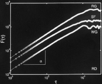
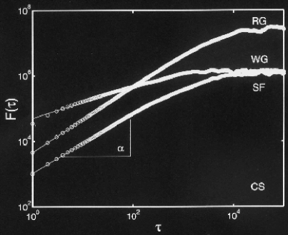
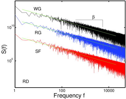
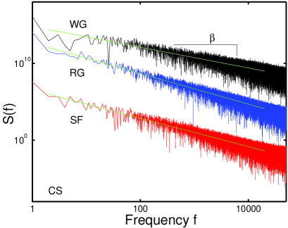
Figure 7: Correlation functions $F(\tau)$ defined in Eq. (16), and power-spectra of the $1/f^{\beta}$ type from Eq. (17), in stationary flow at $R=R^{\star}$ for different network topologies and diffusion rules: random diffusion (RD) and nnn-search (CS). Corresponding exponents are gathered in Table 2. Power spectra have been shifted horizontally for different graphs.

In Fig. 7 correlators $F(\tau)$ and power-spectra $S(f)$ are shown for stationary flow at $R=R^{\star}$ for the three graph topologies and diffusion rules. The corresponding scaling exponents have been obtained by least square fits to the data. Results are found in Table 2. For RD both $\alpha$ and $\beta$ suggest practically uncorrelated workload processes, regardless of the network type. The situation changes for CS where signs for anti-persistence are found in the SF ($\alpha=0.40$, $\beta=1.85$) and especially in the WG ($\alpha=0.21$, $\beta=1.35$).

Observed anti-persistence ($\alpha<1/2$ ) may be related to some kind of regulatory effects due to powerful hubs in the structured networks. As discussed above, the advanced search often directs packets via hub nodes, and even for low global workload, there can emerge long queues at large hub nodes. While waiting in a queue, packets increase the network’s workload, but they do not contribute to randomness of the process. Moreover, when a waiting packet is on turn to be processed, it gets quickly to the target (which is often found in the neighborhood of that hub) and disappears from the traffic; In other words, the system corrects itself by quickly decreasing the workload. Connected with this scenario is the fact that networks with more powerful hubs, such as the WG, are more efficient than networks with only one hub (e.g. SF) or no hubs at all (e.g. RG).

VI Discussion

In this work by use of large-scale numerical simulations and theoretical concepts we demonstrated how packet transport between nodes on different structured networks can be quantified as an anomalous diffusion process. In our model we control both graph topology and microscopic diffusion rules. Our main aim was to explore how topology of graphs affects properties of the diffusion process. For this purpose we ensured a stationary un-jammed flow on each graph topology by an externally fixed posting rate $R$.

We based our work primarily on the analysis of transit-times of packets. We find power-laws in the transit-time distributions which imply non-negligible probabilities for very long delays. We find a marked difference in power-law exponents depending on graph topology and search algorithm. These power-laws are rather independent of the posting rate, suggesting a statistical regularity of the diffusion process that can be related to graph topology when below the jamming transition. For the range of posting rates studied, we find that the particular queuing discipline is of minor importance. The type of queuing is known to play a more important role for larger posting rates where waiting-times of packets increase when approaching the jamming transition. Our main conclusions which characterize the diffusion process on structured networks can be summarized in the following points:

VI.1 Stationarity

We have demonstrated that the traffic of packets on structured networks can be made stationary without imposing any global constraint. We find the stationary jammed flow for a range of values for the posting rate which balances the output rate (number of packets delivered per time step). The output rate strictly depends on the network’s topology and the search algorithm to navigate packets. Generally, for local search algorithms more structured networks, e.g., networks with more powerful hubs and closed cycles have larger output rates. Theoretically, the stationarity of the traffic guarantees that we are dealing with self-similar stochastic processes, which have major advantages for theoretical analysis (scaling).

VI.2 Super-Diffusivity

We found that the traffic of information packets is super-diffusive on any non-trivial graph topology (emergent topologies in evolving networks). In formal terms, this means that distances between nodes in a large graph can be traversed in times that scale sub-quadratically with the graph size (the dynamic exponent $T\sim N^{z}$ is $z<2$). This conclusion remains true even if packets are left to diffuse randomly. This is in marked contrast to random diffusion on space-filling structures, where random diffusion is represented by Brownian motion. Another finding is that in the free-flow regime, differences between graph topologies are marginal when packets diffuse randomly. This underlines the necessity for improving and adapting local diffusion rules in order to optimally use the topology of an underlying graph. To this end we studied transport with the improved local search algorithm which looks for the destination node in next-near-neighbor surrounding of the node.

VI.3 Efficiency

When using the improved local search, transport remains super-diffusive but marked quantitative differences due to graph topologies emerge. The improved local search in combination with some network topologies performs strikingly more efficient than for others. This is especially true for highly structured networks. The efficiency of the network with improved local search is directly related to regulatory effects played by large hub nodes, in particular by the number of hubs and the number of closed cycles. Although the distributions of transit-times of packets in all structured networks are markedly different (generally shorter times in highly structured networks), they still exhibit power-tails.

The optimum strategy for diffusion on a network would be the knowledge of the shortest paths between the initial point and its destination. This knowledge would however require costly global navigation, which is often not available in real networks. Traffic along geodesics may also be inconvenient in the case of queuing, given that in the scale-free graphs a majority of shortest paths pass through hub nodes, while other nodes carry much less traffic. To understand this better we mention that the probability distribution of the number of paths through a node is a fast decaying function $P(u)\sim u^{-2.0}$ in SF and $P(u)\sim u^{-2.27}$ in WG BT_Granada . An advanced local search such as CS is certainly better in this respect, since it disperses the activity over more nodes in the network. This is achieved through the random part of the search, i.e., when the destination node appears not to be in the locally searched nnn area. This feature of the local search implies, however, that some packets may get stuck in remote areas of the network, leading to the long tail in the transit-time distribution.

To improve search algorithms on structured graphs without extending their local character one can think of a statistical improvement which might be realized in many natural systems. To this end one sends multiple copies of the same packet to the same destination. Since all packets move independently and randomly there would be differences between path lengths selected by the different copies. We monitor the shortest transit-time and ignore later arrivals. The first-arrival statistics of multiple copies of the packet is summarized in Fig. 5. It shows that a reasonable improvement is achieved already by sending ten copies of the packet. Statistically, the fastest arriving packets use the minimum path up to four-link separation and longest transit-times are reduced by an order of magnitude compared to the one-copy case. The asymptotic tail has the slope close to 1.9. Similar effects – reduced transit-times by first arrivals – are found in the other two graph topologies, with the slope of the curve practically unchanged, compared to the one-packet distribution. The efficiency of information transport on biological networks – e.g., signaling molecules sent by a node to a particular destination where they can bind chemically – probably utilizes the above statistical methods for improvement. Many identical molecules are being sent from an area of production (e.g. the nucleus) to a target position via a network (cytosceleton).The first arriving molecule binds and chemically acts on the target node. In technological networks the statistical improvement method may be used in low density traffic. For instance, in the stationary flow regime on the Web graph with CS at rate $R\leq 0.04$ one can copy each packet by a factor of ten without yet causing jamming on the network. Other topologies are more sensitive to jamming and the number of copies needs to be adjusted to the basic driving rate $R$.

Maybe our most interesting result is that in several measures (transit-times, $q$ and correlation exponents) we found that neither graph topology nor the search algorithm alone are sufficient to explain for a drastic increase of efficiency of network traffic. We rather find that the combination of both – in form of a good matching – are the source of this improvement. It is most intriguing that for ordinary diffusion very little dependence of network structure was found, meaning for a unguided diffusion no advantage from more structure in a network is gained. In other words either the structure of the network should be adjusted to the processes that the network supports, or the network has to be formed to use these processes most effectively. With this finding it becomes possible to speculate that evolution has adopted certain network structures in nature to cheap and robust search mechanisms, and/or has adapted search strategies to existing networks.

References

- (1) H.K. Lee, H.-W. Lee, D. Kim, Phys. Rev. E 64, 056126 (2001)
- (2) G.B. West, J.H. Brown, B.J Enquist, Science 276, 122-126 (1997).
- (3) K. B. Chong and Y. Choo, physics/0206012.
- (4) J. Abate and W. Whitt, Opns. Res. Lett. 20, 199 (1997).
- (5) Computational Modeling of Genetic and Biochemical Networks, Edited by J.M. Bower and H. Bolouri, MIT Press (cambridge), 2001.
- (6) S. N. Dorogovtsev and J.F.F. Mendes, Evolution of networks, Adv. Phys. 51, 1079 (2002).
- (7) R. Albert and A.-L. Barabási, Rev. Mod. Phys. 74, 47 (2002).
- (8) A. Broder et al., Comput. Networks 33, 309 (2000).
- (9) B. Tadić, Physica A 293, 273 (2001).
- (10) A. Vazquez, R. Pastor-Satorras and A. Vespignani, cond-mat/0112400.
- (11) A. Erramilli, O. Narayan and W. Willinger, IEEE/ACM Trans. Networking 4 209 (1996).
- (12) M. Takayasu, H. Takayasu and T. Sato, Physica A 233 824 (1996).
- (13) B. Tadić and G.J. Rodgers, Adv. Complex Systems, 5, 445 (2002).
- (14) A. Arenas, A. Díaz-Guilera, and R. Guimera, Phys. Rev. Lett. 86, 3196 (2001).
- (15) R. Guimera, A. Díaz-Guilera, F. Vega-Redondo and A. Carbales, cond-mat/0206410.
- (16) R. V. Solé and S. Valverde, Physica A 289, 595 (2001).
- (17) S. Valverde and R. V. Solé, Physica A 312, 636 (2002).
- (18) C. Tsallis, J. Stat. Phys. 52, 479 (1988).
- (19) C. Tsallis and D.J. Bukman, Phys. Rev. E 54, 219 (1996).
- (20) W. Whitt, Stochastic-Process Limits, Springer (NY) 2001.
- (21) B. Tadić, Computer Physics Communications, 147, 586 (2002).
- (22) B. Tadić, Modeling Traffic of Information Packets on Graphs with Complex Topology, to appear in Proceedings of the International Conference of Computational Science, St. Petersburg (2003).
- (23) P.M. Gleiss, P.F. Stadler, A. Wagner, and D.A. Fell, e-print cond-mat/0009124.
- (24) H. Jeong et al., Nature 407, 651 (2000).
- (25) J.C.M. Mombach and J.A. Glazier, Phys. Rev. Lett. 76 (1996) 3032.
- (26) S. Thurner, N. Wick, R. Hanel, R. Sedivy, and L. Huber, Physica A 320C, 475-484 (2003).
- (27) Yu.V. Prohorov and Yu.A. Rozanov, Teoriya Veroyatnostey, Nauka (Moscow) 1973.
- (28) C. Tsallis, R.S. Mendes and R. Plastino, Physica A 261, 534 (1998).
- (29) M. Bologna, C. Tsallis and P. Grigolini, Phys. Rev. E 62 (2000) 2213.
- (30) R. Silva, A.R. Plastino and J.A.S. Lima, Phys. Lett. A 249 (1998) 401.
- (31) A.R. Plastino and A. Plastino, Phys. Lett. A 174 (1993) 384.
- (32) S. Thurner, S.B. Lowen, M.C. Feurstein, C. Heneghan, H.G. Feichtinger, M.C. Teich, Fractals 5, 565-595 (1997).
- (33) E. Koscielny-Bunde, A. Bunde, S. Havlin, H.E. Roman, Y. Goldreich, H.-J. Schellnhuber, Phys. Rev. Lett. 81 729-732 (1998).
- (34) A. Arneodo, E. Bacry, P.V. Graves, J.F. Muzy, Phys.Rev. Lett. 74, 3293-3296 (1995).
- (35) S. Thurner, M.C. Feurstein, M.C. Teich, Phys. Rev. Lett. 81 5688-5691 (1998).
- (36) B. Tadić, Exploring complex graphs by random walks in “Modeling Complex Systems”, P.L. Garrido and J. Marro (Eds.), AIP Conference Proceedings (in press).