Optical Detection of Single-Electron Spin Decoherence in a Quantum Dot

Abstract

We propose a method based on optically detected magnetic resonance (ODMR) to measure the decoherence time $T_{2}$ of a single electron spin in a semiconductor quantum dot. The electron spin resonance (ESR) of a single excess electron on a quantum dot is probed by circularly polarized laser excitation. Due to Pauli blocking, optical excitation is only possible for one of the electron-spin states. The photoluminescence is modulated due to the ESR which enables the measurement of electron-spin decoherence. We study different possible schemes for such an ODMR setup.

I Introduction

Quantum information can be encoded in states of an electron spin $1/2$ in a semiconductor quantum dot.spintronics However, information processing is intrinsically limited by the spin lifetime. For single spins, one distinguishes between two characteristic decay times $T_{1}$ and $T_{2}$. The relaxation of an excited spin state in a magnetic field into the thermal equilibrium is associated with the spin relaxation time $T_{1}$, whereas the spin decoherence time $T_{2}$ is related to the loss of phase coherence of a single spin that is prepared in a superposition of its eigenstates. Experimental $T_{2}$ measurements of single spins in quantum dots are highly desirable because $T_{2}$ is the limiting time scale for coherent spin manipulation.

Recent optical experiments have demonstrated the coherent control and the detection of excitonic states of single quantum dots.gammon1 Nevertheless, the measurement of the $T_{2}$ time of a single electron spin in a quantum dot using optical methods has turned out to be an intricate problem. This is mainly due to the interaction of the electron and the hole inside an exciton.current The electron and hole spin are decoupled only if the hole spin couples (via spin-orbit interaction) stronger to the environment than to the electron spin. Recent experiments, measuring Faraday rotation, have suggested that this is not the case for excitons in quantum dots.guptaT2 Alternatively, if electron-hole pairs are excited inside the barrier material of a quantum dot heterostructure, the carriers diffuse after their creation to the dots and are captured inside them within typically tens of picoseconds.ohnesorge ; raymond By that time, electron and hole spins have decoupled. In such an experiment, the Hanle effect would allow the measurement of electron-spin decoherence. However, this approachepstein has not yet given conclusive results for $T_{2}$.

What is a promising approach to measure the electron-spin decoherence time $T_{2}$ by optical methods? For this, initially some coherence of the electron spin must be produced, preferably in the absence of holes. This can be done using electron spin resonance (ESR). The coherence decays and, after some time, the remaining coherence is measured optically. This implies using optically detected magnetic resonance (ODMR). ODMR schemes have, e.g., been applied to measure the spin coherence of single nitrogen-vacancy centers in diamond.gruber For quantum dots, ODMR has recently been applied to electrons and holes in CdSe dotsLifshitz and to excitons in InAs/GaAs dots.zurauskiene While these two experiments have not considered single spin coherence, the feasibility of the combination of ESR and optical methods in quantum dot experiments has been demonstrated.

In this work, we make use of Pauli blocking of exciton creationpauliblocking in an ODMR setup. We show that the linewidth of the photoluminescence as a function of the ESR field frequency provides a lower bound on $T_{2}$. Further, if pulsed laser and cw ESR excitation are applied, electron spin Rabi oscillations can be detected via the photoluminescence.

We consider quantum dots which confine electrons as well as holes (type I dots). We assume a ground state where the dot is charged with one single electron. This can be achieved, e.g., by $n$ dopingcortez or by electrical injection.abstreiter2 Such a single-electron state can be optically excited, which leads to the formation of a negatively charged exciton, consisting of two electrons and one hole. Recent experiments on InAs dotstrion1 ; trion2 and GaAs dotstrion3 have shown that in the charged exciton ground state, the two electrons form a spin singlet in the lowest (conduction-band) electron level and the hole occupies the lowest (valence-band) hole level. Note that single-electron level spacings can be relatively large, e.g., on the order of 50 meV for InAs dots.fricke Typically, the level spacing of confined hole states is smaller than the one of electrons.schmidt We assume that the lowest heavy hole (hh) (with total angular momentum projection $J_{z}\!=\!\pm 3/2$) and light hole (lh) ($J_{z}\!=\!\pm 1/2$) dot levels are split by an energy $\delta_{hh-lh}$. Additionally, mixing of hh and lh states should be negligible.mixing These conditions are satisfied for several types of quantum dots.trion1 ; trion2 ; trion3 ; efrosCdSe ; efros2 Then, circularly polarized optical excitation that is restricted to either hh or lh states excites spin-polarized electrons. In this work, we first assume a hh ground state for holes. We discuss then different hole configurations.

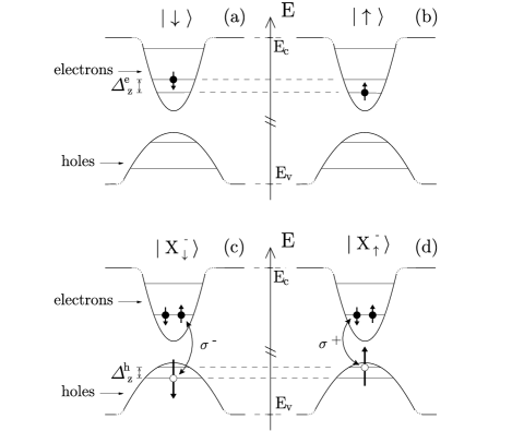
Figure 1: The states of a single quantum dot in a static magnetic field, (a) $|\!\downarrow\rangle$, (b) $|\!\uparrow\rangle$, (c) $|X_{\downarrow}^{-}\rangle$, and (d) $|X_{\uparrow}^{-}\rangle$. The Zeeman splittings are $\Delta_{z}^{e}=g_{e}^{z}{\mu_{\mathrm{B}}}B_{z}$ for the electron and $\Delta_{z}^{h}=g_{hh}^{z}{\mu_{\mathrm{B}}}B_{z}$ for the hole. Coherent transitions occur between (a) and (b) due to the ESR field and between (a) and (c) due to the $\sigma^{-}$-polarized laser field. The arrows in (c) and (d) indicate which electron-hole pair couples with the photon field of polarization $\sigma^{\pm}$.

The states of a quantum dot can be taken as follows; see also Fig. 1. A single electron in the lowest orbital state is either in the spin ground state $|\!\uparrow\rangle$ or in the excited spin state $|\!\downarrow\rangle$. Adding an electron-hole pair, the negatively charged exciton (in the orbital ground state) is either in the excited spin state $|X_{\downarrow}^{-}\rangle$ or in the spin ground state $|X_{\uparrow}^{-}\rangle$. For these excitonic states, the subscripts $\downarrow,\uparrow$ refer to the hh spin and we apply the usual time-inverted notation for hole spins. For simplicity, we assume $\mathrm{sign}(g_{e}^{z})=\mathrm{sign}\left(g_{hh}^{z}\right)$ for the electron and the hh $g$ factors in $z$ direction. Note that the very same scheme can also be applied if the sign of $g_{hh}^{z}$ is reversed. Then, one would use a $\sigma^{+}$ laser field and all results apply after interchanging $|X_{\downarrow}^{-}\rangle$ and $|X_{\uparrow}^{-}\rangle$.

II Hamiltonian

We describe the coherent dynamics of a quantum dot, charged with a single excess electron, in this ODMR setup with the Hamiltonian

$$H=H_{\mathrm{dot}}+H_{\mathrm{ESR}}+H_{\mathrm{L}}+H_{\mathrm{d-L}},$$ (1)

coupling the three states $|\!\uparrow\rangle$, $|\!\downarrow\rangle$, and $|X_{\downarrow}^{-}\rangle$. Here, $H_{\mathrm{dot}}$ comprises the quantum dot potential, the Zeeman energies due to a constant magnetic field in $z$ direction, and the Coulomb interaction of electrons and holes. It defines the dot energy $E_{n}$ by $H_{\mathrm{dot}}|n\rangle=E_{n}|n\rangle$. Here, the electron Zeeman splitting is $g_{e}^{z}{\mu_{\mathrm{B}}}B_{z}=E_{\downarrow}-E_{\uparrow}$, where ${\mu_{\mathrm{B}}}$ is the Bohr magneton.overhauser The ESR term $H_{\mathrm{ESR}}(t)$ couples $|\!\uparrow\rangle$ and $|\!\downarrow\rangle$ via $\mathbf{B}_{\perp}(t)$, which rotates with frequency $\omega_{\mathrm{ESR}}$ in the $xy$ plane.linESR ; engel The ESR Rabi frequency is $\Omega_{\mathrm{ESR}}=g_{e}^{\perp}{\mu_{\mathrm{B}}}B_{\perp}$, with $g$ factor $g_{e}^{\perp}$. Even if the ESR field is also resonant with the hole Zeeman splitting, it has a negligible effect on the charged exciton states since they recombine quickly. An oscillating field ${\mu_{\mathrm{B}}}\tensor{\mathbf{g}}\mathbf{B}$ can also be produced with voltage-controlled modulation of the electron $g$ tensor $\tensor{\mathbf{g}}$.kato A $\sigma^{-}$-polarized laser beam is applied in $z$ direction (typically parallel to $[001]$), with free laser field Hamiltonian $H_{\mathrm{L}}=\omega_{\mathrm{L}}a_{\mathrm{L}}^{\dagger}a_{\mathrm{L}}$, where the laser frequency is $\omega_{\mathrm{L}}$, $a_{\mathrm{L}}^{(\dagger)}$are photon operators, and we set $\hbar=1$. The coupling of $|\!\downarrow\rangle$ and $|X_{\downarrow}^{-}\rangle$ to the laser field is described by $H_{\mathrm{d}-\mathrm{L}}$ which introduces the complex optical Rabi frequency $\Omega_{\mathrm{L}}$.optRabi Since the dot is only coupled to a single circularly polarized laser mode via $H_{\mathrm{d-L}}$, the terms that violate energy conservation vanish due to selection rules. If the laser bandwidth is smaller than $\delta_{hh-lh}$, the absorption of a $\sigma^{-}$ photon in the spin ground state $|\!\uparrow\rangle$ is excluded due to Pauli blocking.trionexc We neglect all multi-photon processes via other levels since they are only relevant to high-intensity laser fields. For this configuration, the $\sigma^{-}$ photon absorption is switched “on” and “off” by the ESR-induced electron-spin flips. Here, the laser bandwidth and the temperature can safely exceed the electron Zeeman splitting. We transform $H$ into the rotating frame with respect to $\omega_{\mathrm{ESR}}$ and $\omega_{\mathrm{L}}$. The laser detuning is $\delta_{\mathrm{L}}=(E_{X\downarrow}-E_{\downarrow})-\omega_{\mathrm{L}}$ and the ESR detuning $\delta_{\mathrm{ESR}}=g_{e}^{z}{\mu_{\mathrm{B}}}B_{z}-\omega_{\mathrm{ESR}}$.

III Generalized Master Equation

We next consider the reduced density matrix for the dot, $\rho={{\mathrm{Tr}}_{\mathrm{R}}\,}\rho_{\mathrm{F}}$, where $\rho_{\mathrm{F}}$ is the full density matrix and ${{\mathrm{Tr}}_{\mathrm{R}}\,}$ is the trace taken over the environment (or reservoir). In the von Neumann equation $\dot{\rho}_{\mathrm{F}}=-i\left[H,\,\rho_{\mathrm{F}}\right]$, we treat the interaction with the ESR and laser fields exactly with the Hamiltonian in the rotating frame. We describe the coupling with the environment (radiation field, nuclear spins, phonons, spin-orbit interaction, etc.) with phenomenological rates. We write $W_{nm}\equiv W_{n\leftarrow m}$ for (incoherent) transitions from state $|m\rangle$ to $|n\rangle$ and $V_{nm}$ for the decay of off-diagonal elements of $\rho$. Note that usually $V_{nm}\geq\frac{1}{2}\sum_{k}\left(W_{kn}+W_{km}\right)$. The electron-spin relaxation timekimble is $T_{1}=\left(W_{{\uparrow\downarrow}}+W_{{\downarrow\uparrow}}\right)^{-1}$, with spin-flip rates $W_{{\uparrow\downarrow}}$ and $W_{{\downarrow\uparrow}}$. In the absence of the ESR and laser excitations, the off-diagonal matrix elements of the electron spin decay with the (intrinsic) single-spin decoherence rate $V_{{\downarrow\uparrow}}=1/T_{2}$. The linewidth of the optical $\sigma^{-}$ transition is denoted by $V_{\mathrm{X}}=V_{X\downarrow,\downarrow}$. We use the notation $\rho_{n}=\langle n|\rho|n\rangle$ and $\rho_{nm}=\langle n|\rho|m\rangle$. The master equation is given in the rotated basis $|\!\uparrow\rangle$, $|\!\downarrow\rangle$, $|X_{\uparrow}^{-}\rangle$, $|X_{\downarrow}^{-}\rangle$ as $\dot{\rho}=\mathcal{M}\rho$, where $\mathcal{M}$ is a superoperator. Explicitly,

$${{\dot{\rho}_{\uparrow}}} = \Omega_{\mathrm{ESR}}{\textrm{Im}}\rho_{{\downarrow\uparrow}}\!+\!W_{\mathrm{em}}\rho_{X\uparrow}\!+\!W_{{\uparrow\downarrow}}{\rho_{\downarrow}}\!-\!W_{{\downarrow\uparrow}}{\rho_{\uparrow}},$$ (2)

$${{\dot{\rho}_{\downarrow}}} = -\Omega_{\mathrm{ESR}}{\textrm{Im}}\rho_{{\downarrow\uparrow}}+{\textrm{Im}}(\Omega_{\mathrm{L}}^{*}\rho_{X\downarrow,\downarrow})+W_{\mathrm{em}}\,\rho_{X\downarrow}$$ (3)

$$+W_{{\downarrow\uparrow}}\,{\rho_{\uparrow}}-W_{{\uparrow\downarrow}}\,{\rho_{\downarrow}},$$

$$\dot{\rho}_{X\downarrow} = -{\textrm{Im}}(\Omega_{\mathrm{L}}^{*}\rho_{X\downarrow,\downarrow})+W_{X\downarrow,X\uparrow}\,\rho_{X\uparrow}$$ (4)

$$-\left(W_{\mathrm{em}}+W_{X\uparrow,X\downarrow}\right)\rho_{X\downarrow},$$

$$\dot{\rho}_{X\uparrow} = W_{X\uparrow,X\downarrow}\,\rho_{X\downarrow}-\left(W_{\mathrm{em}}+W_{X\downarrow,X\uparrow}\right)\rho_{X\uparrow},$$ (5)

$${{\dot{\rho}_{{\downarrow\uparrow}}}} = \frac{i}{2}\Omega_{\mathrm{ESR}}\left({\rho_{\downarrow}}-{\rho_{\uparrow}}\right)-\frac{i}{2}\Omega_{\mathrm{L}}^{*}\rho_{X\downarrow,\uparrow}$$ (6)

$$-\left(i\delta_{\mathrm{ESR}}+T_{2}^{-1}\right)\,\rho_{{\downarrow\uparrow}},$$

$$\dot{\rho}_{X\downarrow,\uparrow} = \frac{i}{2}\Omega_{\mathrm{ESR}}\,\rho_{X\downarrow,\downarrow}-\frac{i}{2}\Omega_{\mathrm{L}}\rho_{{\downarrow\uparrow}}$$ (7)

$$-[i(\delta_{\mathrm{ESR}}+\delta_{\mathrm{L}})+V_{X\downarrow,\uparrow}]\,\rho_{X\downarrow,\uparrow},$$

$$\dot{\rho}_{X\downarrow,\downarrow} = \frac{i}{2}\Omega_{\mathrm{ESR}}\rho_{X\downarrow,\uparrow}-\frac{i}{2}\Omega_{\mathrm{L}}({\rho_{\downarrow}}-\rho_{X\downarrow})$$ (8)

$$-(i\delta_{\mathrm{L}}+V_{\mathrm{X}})\rho_{X\downarrow,\downarrow}.$$

The remaining matrix elements of $\rho$ are decoupled and are not important here.

Figure 2: Scheme of the transitions between $|\!\uparrow\rangle$, $|\!\downarrow\rangle$, $|X_{\uparrow}^{-}\rangle$, and $|X_{\downarrow}^{-}\rangle$. Wavy arrows describe the transitions driven by the ESR field and the laser field with frequencies $\omega_{\mathrm{ESR}}$ and $\omega_{\mathrm{L}}$, respectively. The corresponding Rabi frequencies are $\Omega_{\mathrm{ESR}}$ and $|\Omega_{\mathrm{L}}|$. A detuning $\delta_{\mathrm{ESR}}=\Delta_{z}^{e}-\omega_{\mathrm{ESR}}$ is shown for the ESR field, with Zeeman splitting $\Delta_{z}^{e}$. Incoherent transitions are depicted with arrows and occur at rates $W_{nm}$. We consider $W_{\downarrow,X\downarrow}=W_{\uparrow,X\uparrow}=:W_{\mathrm{em}}$.

IV ESR Linewidth in Photoluminescence

We first consider the photoluminescence for a cw ESR and laser field. For this, we calculate the stationary density matrix $\bar{\rho}$ with $\dot{\bar{\rho}}=0$. We introduce the rate

$$W_{\mathrm{L}}=\frac{|\Omega_{\mathrm{L}}|^{2}}{2}\>\frac{V_{\mathrm{X}}}{V_{\mathrm{X}}^{2}+\delta_{\mathrm{L}}^{2}}$$ (9)

for the optical excitation, with maximum value $W_{\mathrm{L}}^{\mathrm{max}}$ at $\delta_{\mathrm{L}}=0$. We first solve $\dot{\bar{\rho}}_{X\downarrow,\uparrow}=0$ and find that the coupling to the laser field produces an additional decoherence channel to the electron spin. We obtain the renormalized spin decoherence rate $V_{\mathrm{ESR}}$ which satisfies

$$V_{\mathrm{ESR}}\leq\frac{1}{T_{2}}+\frac{|\Omega_{\mathrm{L}}|^{2}}{4V_{X\downarrow,\uparrow}}\approx\frac{1}{T_{2}}+\frac{1}{2}W_{\mathrm{L}}^{\mathrm{max}}.$$ (10)

Further, the ESR detuning is also renormalized,

$$\tilde{\delta}_{\mathrm{ESR}}\geq\delta_{\mathrm{ESR}}\left[1-\frac{|\Omega_{\mathrm{L}}|^{2}}{\left(W_{\mathrm{em}}+W_{X\uparrow,X\downarrow}\right)^{2}}\right].$$ (11)

We assume that these renormalizations and $\delta_{\mathrm{L}}$ are small compared to the linewidth of the optical transition, i.e., $W_{\mathrm{L}}^{\mathrm{max}},\,|\tilde{\delta}_{\mathrm{ESR}}-\delta_{\mathrm{ESR}}|<V_{\mathrm{X}}$. Then, if both transitions are near resonance, $\delta_{\mathrm{L}}\lesssim V_{\mathrm{X}}$ and $|\tilde{\delta}_{\mathrm{ESR}}|\lesssim V_{\mathrm{ESR}}$, no additional terms appear in the renormalized master equation. We solve $\dot{\bar{\rho}}_{X\downarrow,\downarrow}=0$ and $\dot{\bar{\rho}}_{{\uparrow\downarrow}}=0$ and introduce the rate

$$W_{\mathrm{ESR}}=\frac{\Omega_{\mathrm{ESR}}^{2}}{2}\>\frac{V_{\mathrm{ESR}}}{{V_{\mathrm{ESR}}}^{2}+{\tilde{\delta}_{\mathrm{ESR}}}^{2}},$$ (12)

which together with $W_{\mathrm{L}}$ eliminates $\Omega_{\mathrm{L}}$, $V_{\mathrm{X}}$, $\delta_{\mathrm{L}}$, $\Omega_{\mathrm{ESR}}$, $V_{\mathrm{ESR}}$, and $\tilde{\delta}_{\mathrm{ESR}}$ from the remaining equations for the diagonal elements of $\rho$. These now contain the effective spin-flip rates $\tilde{W}_{{\uparrow\downarrow}}=W_{{\uparrow\downarrow}}+W_{\mathrm{ESR}}$ and $\tilde{W}_{{\downarrow\uparrow}}=W_{{\downarrow\uparrow}}+W_{\mathrm{ESR}}$.

Figure 3: The total photoluminescence rate $\Gamma$ is a Lorentzian as a function of the ESR detuning $\tilde{\delta}_{\mathrm{ESR}}$. Its linewidth $w$ gives an upper bound for $2/T_{2}$. Here, we use $g_{e}=0.5$, $B_{\perp}=1\>\mathrm{G}$, $T_{2}=100\>\mathrm{ns}$, $W_{{\uparrow\downarrow}}=W_{{\downarrow\uparrow}}=(20\>\mathrm{\mu s})^{-1}$, $W_{\mathrm{em}}=10^{9}\>\mathrm{s^{-1}}$, $W_{X\uparrow,X\downarrow}=W_{X\downarrow,X\uparrow}=W_{\mathrm{em}}/2$, $\delta_{\mathrm{L}}=0$, $V_{X\downarrow,\uparrow}=V_{\mathrm{X}}=(W_{\mathrm{em}}+W_{X\uparrow,X\downarrow})/2$, and $\Omega_{\mathrm{L}}=2\Omega_{\mathrm{ESR}}\sqrt{T_{2}V_{\mathrm{X}}}$. With these parameters, the requirement $W_{\mathrm{L}}\lesssim T_{2}^{-1}\lesssim V_{\mathrm{ESR}}$ is satisfied.

We find the stationary solution

$$\bar{\rho}_{\uparrow} = \eta\,W_{\mathrm{L}}\,W_{\mathrm{em}}\,W_{X\uparrow,X\downarrow}+\eta\,\tilde{W}_{{\uparrow\downarrow}}\,W_{\mathrm{em}}\,W_{X\uparrow,X\downarrow}$$ (13)

$$\;+\eta\,\tilde{W}_{{\uparrow\downarrow}}\left(W_{\mathrm{L}}+W_{\mathrm{em}}\right)\,\left(W_{\mathrm{em}}+W_{X\downarrow,X\uparrow}\right),\qquad$$

$$\bar{\rho}_{\downarrow} = \eta\,\tilde{W}_{{\downarrow\uparrow}}\,\left(W_{\mathrm{L}}+W_{\mathrm{em}}\right)\left(W_{\mathrm{em}}+W_{X\downarrow,X\uparrow}\right)$$ (14)

$$\;+\eta\,\tilde{W}_{{\downarrow\uparrow}}\,W_{\mathrm{em}}\,W_{X\uparrow,X\downarrow},$$

$$\bar{\rho}_{X\downarrow} = \eta\,W_{\mathrm{L}}\,\tilde{W}_{{\downarrow\uparrow}}\,\left(W_{\mathrm{em}}+W_{X\downarrow,X\uparrow}\right),$$ (15)

$$\bar{\rho}_{X\uparrow} = \eta\,W_{\mathrm{L}}\,\tilde{W}_{{\downarrow\uparrow}}\,W_{X\uparrow,X\downarrow},$$ (16)

where the normalization factor $\eta$ is such that $\sum_{n}\rho_{n}=1$. Note that $\bar{\rho}_{\uparrow}\geq\bar{\rho}_{\downarrow}$ is satisfied for $W_{{\uparrow\downarrow}}\geq W_{{\downarrow\uparrow}}$. Thus, electron-spin polarization is achieved due to the hole-spin relaxation channel, analogous to an optical pumping scheme. Now, photons with $\sigma^{-}$ ($\sigma^{+}$) polarization are emitted from the dot at the rate $\Gamma^{-}=W_{\mathrm{em}}\bar{\rho}_{X\downarrow}$ ($\Gamma^{+}=W_{\mathrm{em}}\bar{\rho}_{X\uparrow}$). These rates are proportional to $W_{\mathrm{ESR}}/(\gamma+W_{\mathrm{ESR}})$ for a given $\gamma$, up to a constant background which is negligible for $W_{{\downarrow\uparrow}}<W_{\mathrm{ESR}}$. In particular, the total rate $\Gamma=\Gamma^{-}+\Gamma^{+}$ as a function of $\tilde{\delta}_{\mathrm{ESR}}$ is a Lorentzian with linewidth

$$w=2\,V_{\mathrm{ESR}}\sqrt{1+\frac{W_{\mathrm{ESR}}^{\mathrm{max}}}{\gamma}};$$ (17)

see Fig. 3. Analyzing the expression for $\gamma$, we find the relevant parameter regime with the inequality

$$w \leq 2\,V_{\mathrm{ESR}}\,\Bigg{[}1+\frac{2\,W_{\mathrm{ESR}}^{\mathrm{max}}}{W_{\mathrm{L}}}\,\left(1+\frac{W_{\mathrm{em}}}{W_{\mathrm{r}}}+\frac{W_{X\downarrow,X\uparrow}}{W_{\mathrm{r}}}\right)$$ (18)

$$\quad+\frac{3\,W_{\mathrm{ESR}}^{\mathrm{max}}}{W_{\mathrm{r}}}+\frac{W_{\mathrm{ESR}}^{\mathrm{max}}}{W_{\mathrm{em}}}\,\left(1+\frac{3\,W_{X\downarrow,X\uparrow}}{W_{\mathrm{r}}}\right)\Bigg{]}^{1/2}\!\!\!\!\!\!\!,$$

which saturates for vanishing $W_{{\downarrow\uparrow}}$ and $W_{{\uparrow\downarrow}}$. Here, the rate $W_{\mathrm{r}}=W_{X\uparrow,X\downarrow}+W_{{\uparrow\downarrow}}\left(1+W_{\mathrm{em}}/W_{\mathrm{L}}\right)$ describes different relaxation channels, all leading to the ground state $|\!\uparrow\rangle$, and thus corresponds to “switching off” the laser excitations. If $W_{\mathrm{r}}$ is large, e.g., due to efficient hole-spin relaxation,Flissikowski $w\approx 2\,V_{\mathrm{ESR}}$. From the linewidth $w$ one can extract a lower bound for $T_{2}$: $T_{2}\geq 1/V_{\mathrm{ESR}}\geq 2/w$. Further, this lower bound saturates when the expression in brackets in Eq. (18) becomes close to 1 and $T_{2}^{-1}\approx V_{\mathrm{ESR}}$ [see Eq. (10)], i.e., the $T_{2}$ time is given by the linewidth. Comparing with the exact solution, we find that our analytical approximation gives the value of $\Gamma$ within $0.2\%$ for the parameters of Fig.  3. Due to possible imperfections in this ODMR scheme, e.g., mixing of hh and lh states or a small contribution of the $\sigma^{+}$ polarization in the laser light, also the state $|\!\uparrow\rangle$ can be optically excited. We describe this with the effective rate $W_{\mathrm{L},\uparrow}$ which leads to an additional linewidth broadening [similar to Eq. (18)]. This effect is small for $W_{\mathrm{L},\uparrow}<W_{\mathrm{ESR}}$. Detection of the laser stray light can be avoided by only measuring $\Gamma^{+}$. Otherwise, the laser could be distinguished from $\Gamma^{-}$ by using two-photon absorption. As an alternative, the optical excitation could be tuned to an excited hole state (hh or lh), possibly with a reversal of laser polarization. A pulsed laser, finally, would enable the distinction between luminescence and laser light by time gated detection.

Figure 4: Average number $N$ of photons emitted per period $\tau_{\mathrm{rep}}$ as function of the laser pulse repetition time for (a) $\pi$ pulses with $\Delta t=5\,\mathrm{ps}$ and $\Omega_{\mathrm{L}}=\pi/\Delta t$, and (b) pulses with $\Delta t=20\,\mathrm{ns}$ and $\Omega_{\mathrm{L}}=\pi/(500\,\mathrm{ps})$. We have set $\delta_{\mathrm{ESR}}=0$. The other parameters are the same as in Fig. 3. The decay of the oscillation is given by $V_{\mathrm{ESR}}$ and therefore depends on $T_{2}$.

V Spin Rabi Oscillations via Photoluminescence

For a pulsed $\sigma^{-}$ laser, one can also measure $\Gamma$ as a function of the pulse repetition time $\tau_{\mathrm{rep}}$ instead of $\tilde{\delta}_{\mathrm{ESR}}$. We still use cw ESR (or, alternatively, a static transverse magnetic field, i.e., in the Voigt geometry). We stress that the same restrictions on the laser bandwidth as in the cw case apply. Due to hole spin flips, followed by emission of a photon, the dot is preferably in the state $|\!\uparrow\rangle$ rather than $|\!\downarrow\rangle$ at the end of a laser pulse. The magnetic field then acts on the electron spin until the next laser pulse arrives. Finally, the spin state $|\!\downarrow\rangle$ is read out optically and, therefore, the Rabi oscillations (or spin precessions) can be observed in the photoluminescence as function of $\tau_{\mathrm{rep}}$; see Fig. 4. For simplicity, we consider square pulses of length $\Delta t$. We write in the master equation $\mathcal{M}(t)=\mathcal{M}_{\mathrm{L}}$ during a laser pulse and otherwise $\mathcal{M}(t)=\mathcal{M}_{0}$, setting $\Omega_{\mathrm{L}}=0$. We find the steady-state density matrix $\rho_{\infty}$ of the dot just after the pulse with $U_{p}\rho_{\infty}=\rho_{\infty}$, where $U_{p}=\exp(\mathcal{M}_{\mathrm{L}}\Delta t)\exp[\mathcal{M}_{0}(\tau_{\mathrm{rep}}-\Delta t)]$ describes the time evolution during $\tau_{\mathrm{rep}}$.

The photoluminescence rate is now evaluated by $\Gamma=W_{\mathrm{em}}\overline{(\rho_{X\downarrow}+\rho_{X\uparrow})}$, where the bar designates time averaging over many periods $\tau_{\mathrm{rep}}$. For $\Delta t\geq\pi/\Omega_{\mathrm{L}},\,W_{\mathrm{em}}^{-1}$, the spin oscillations become more pronounced; see Fig. 4 (b). This results from an enhanced relaxation to the state $|\!\uparrow\rangle$ during each pulse and thus from a much larger $\rho_{\uparrow}$ than $\rho_{\downarrow}$ just after the pulse.

VI Conclusions

We have proposed an ODMR setup with ESR and polarized optical excitation. We have shown that this setup allows the optical measurement of the single-electron spin decoherence time $T_{2}$ in semiconductor quantum dots. The discussed cw and pulsed optical detection schemes can also be combined with pulsed instead of cw ESR, allowing spin echo and similar standard techniques. Such pulses can, e.g., be produced via the ac Stark effect.ACstark Further, as an alternative to photoluminescence detection, photocurrent can be used to read out the charged exciton,abstreiter2 and the same ODMR scheme can be applied.

References

• (1) Semiconductor Spintronics and Quantum Computation, edited by D.D. Awschalom, D. Loss, and N. Samarth, Series on Nanoscience and Technology, Vol.Β XVI (Springer, New York, 2002).
• (2) N.H. Bonadeo, J. Erland, D. Gammon, , D. Park, D.S. Katzer and D.G. Steel, Science 282, 1473 (1998).
• (3) Alternatively, one can measure $T_{2}$ via currents through quantum dots in an ESR field (Refs.Β 24 and 31). However, using an optical detection scheme there is no need for contacting dots with current leads (thus reducing decoherence) and one can benefit from the high sensitivity of photodetectors.
• (4) J.A. Gupta, D.D. Awschalom, X. Peng, and A.P. Alivisatos, Phys.Β Rev.Β B 59, R10 421 (1999).
• (5) B. Ohnesorge, M. Albrecht, J. Oshinowo, A. Forchel, and Y. Arakawa, Phys.Β Rev.Β B 54, 11 532 (1996).
• (6) S. Raymond, S. Fafard, P.J. Poole, A. Wojs, P. Hawrylak, S. Charbonneau, D. Leonard, R. Leon, P.M. Petroff, and J.L. Merz, Phys.Β Rev.Β B 54, 11 548 (1996).
• (7) R.J. Epstein, D.T. Fuchs, W.V. Schoenfeld, P.M. Petroff, and D.D. Awschalom, Appl.Β Phys.Β Lett.Β 78, 733 (2001).
• (8) A. Gruber, A. DrΓ€benstedt, C. Tietz, L. Fleury, J. Wrachtrup, and C. von Borczyskowski, Science 276, 2012 (1997); F. Jelezko, T. Gaebel, I. Popa, A. Gruber, and J. Wrachtrup, Phys.Β  Rev.Β  Lett.Β  92, 076401 (2004); for a recent work on ensembles, see F.T. Charnock and T.A. Kennedy, Phys.Β Rev.Β B 64, 041201 (2001).
• (9) E. Lifshitz, I. Dag, I.D. Litvitn, and G. Hodes, J.Β Phys.Β Chem.Β B 102, 9245 (1998).
• (10) N. Zurauskiene, G. Janssen, E. Goovaerts, A. Bouwen, D. Shoemaker, P.M. Koenraad, and J.H. Wolter, Phys.Β  status solidi B 224, 551 (2001).
• (11) For a recent discussion, see, e.g., T. Calarco, A. Datta, P. Fedichev, E. Pazy, and P. Zoller, Phys.Β Rev.Β A 68, 012310 (2003).
• (12) S. Cortez, O. Krebs, S. Laurent, M. Senes, X. Marie, P. Voisin, R. Ferreira, G. Bastard, J.M. GΓ©rard, and T. Amand, Phys.Β  Rev.Β  Lett.Β  89, 207401 (2002).
• (13) M. Baier, F. Findeis, A. Zrenner, M. Bichler, and G. Abstreiter, Phys.Β Rev.Β B 64, 195326 (2001).
• (14) M. Bayer, G. Ortner, O. Stern, A. Kuther, A.A. Gorbunov, A. Forchel, P. Hawrylak, S. Fafard, K. Hinzer, T.L. Reinecke, S.N. Walck, J.P. Reithmaier, F. Klopf, and F. SchΓ€fer, Phys.Β Rev.Β B 65, 195315 (2002).
• (15) J.J. Finley, D.J. Mowbray, M.S. Skolnick, A.D. Ashmore, C. Baker, A.F.G. Monte, and M. Hopkinson, Phys.Β Rev.Β B 66, 153316 (2002).
• (16) J.G. Tischler, A.S. Bracker, D. Gammon, and D. Park, Phys.Β Rev.Β B 66, 081310 (2002).
• (17) M. Fricke, A. Lorke, J.P. Kotthaus, G. Medeiros-Ribeiro, and P.M. Petroff, Europhys.Β  Lett.Β  36, 197 (1996).
• (18) K.H. Schmidt, G. Medeiros-Ribeiro, M. Oestreich, P.M. Petroff, and G.H. DΓΆhler, Phys.Β Rev.Β B 54, 11 346 (1996).
• (19) For dot shapes of lower than circular symmetry, mixing of different band states can become significant. See, e.g., L.-W. Wang, J. Kim, and A. Zunger, Phys.Β Rev.Β B 59, 5678 (1999).
• (20) Al.L. Efros, Phys.Β Rev.Β B 46, 7448 (1992).
• (21) Al.L. Efros and A.V. Rodina, Phys.Β Rev.Β B 47, 10 005 (1993).
• (22) In $B_{z}$, we have absorbed the Overhauser field which could possibly arise from dynamically polarized nuclear spins.
• (23) A linearly oscillating magnetic field, $\mathbf{B}_{x}(t)=B_{x}^{0}\cos(\omega_{\mathrm{ESR}}t)\mathbf{\hat{x}}$, can also be applied, cf. J.J. Sakurai, Modern Quantum Mechanics, (Addison-Wesley, Reading, MA, 1995), Revised Edition. This leads, in the rotating wave approximation (RWA), to the same result as the rotating field for $B_{\perp}\rightarrow B_{x}^{0}/2$.
• (24) H.-A. Engel and D. Loss, Phys.Β Rev.Β Lett.Β 86, 4648 (2001); Phys.Β Rev.Β B 65, 195321 (2002).
• (25) Y. Kato, R.C. Myers, D.C. Driscoll, A.C. Gossard, J. Levy, and D.D. Awschalom, Science 299, 1201 (2003).
• (26) We use the standard description $H_{\mathrm{d}-\mathrm{L}}\!=\!-e\mathbf{A}\!\cdot\!\mathbf{p}/m_{0}c$, with vector potential $\mathbf{A}$ and charge $e$, bare mass $m_{0}$, and momentum $\mathbf{p}$ of the electron. Since excitonic electric fields are present, we neglect the typically smaller electric fields of the laser that are contained in second order in the term $\propto\mathbf{A}^{2}$. We apply the electric dipole approximation and assume a coherent photon state for the laser. Then, $\Omega_{\mathrm{L}}\!=\!\alpha e\langle X_{\downarrow}^{-}|\mathbf{e}_{\mathrm{L}}\!\cdot\!\mathbf{p}|\!\downarrow\rangle\sqrt{{2\hbar/m_{0}^{2}c^{2}V\epsilon_{0}\epsilon_{r}\omega_{\mathrm{L}}}}$, with volume $V$, unit polarization vector $\mathbf{e}_{\mathrm{L}}$, and mean photon number $|\alpha|^{2}$ of the laser mode. The relative permittivity of the semiconductor is $\epsilon_{r}$, and $\epsilon_{0}$ is the dielectric constant. See also L. Mandel and E. Wolf, Optical Coherence and Quantum Optics (Cambridge University Press, Cambridge, 1995).
• (27) Excitation of a charged exciton state containing an electron triplet would require an additional energy of $\sim 40$ meV (Ref.Β 12) and can be excluded by the low laser bandwidth.
• (28) The single-spin relaxation time $T_{1}$ can be measured via a similar double resonance scheme as discussed in this work. For this, we assume that the laser polarization is $\sigma^{+}$ and the temperature is sufficiently low that $|X_{\downarrow}^{-}\rangle$ is decoupled from the three-level system $|\!\uparrow\rangle$, $|\!\downarrow\rangle$, and $|X_{\uparrow}^{-}\rangle$, cf. Figs.Β 1 and 2. In the regime $\Omega_{\mathrm{L}},\,W_{\mathrm{em}}\gg\Omega_{\mathrm{ESR}},\,W_{{\uparrow\downarrow}}$, the mean time of fluorescence interruptions due to ESR excitation provides $T_{1}$, similarly as for a single atom [H.J. Kimble, R.J. Cook, and A.L. Wells, Phys.Β Rev.Β A 34, 3190 (1986)].
• (29) T. Flissikowski, I.A. Akimov, A. Hundt, and F. Henneberger, Phys.Β Rev.Β B 68, R161309 (2003); L.M. Woods, T.L. Reinecke, and R. Kotlyar, Phys.Β Rev.Β B 69, 125330 (2004).
• (30) J.A. Gupta, R. Knobel, N. Samarth, and D.D. Awschalom, Science 292, 2458 (2001); C.E. Pryor and M.E. FlattΓ© (unpublished), quant-ph/0211160.
• (31) I. Martin, D. Mozyrsky, and H.W. Jiang, Phys.Β Rev.Β Lett.Β 90, 018301 (2003).