Adiabatic loading of bosons into optical lattices

Abstract

The entropy-temperature curves are calculated for non-interacting bosons in a 3D optical lattice and a 2D lattice with transverse harmonic confinement for ranges of depths and filling factors relevant to current experiments. We demonstrate regimes where the atomic sample can be significantly heated or cooled by adiabatically changing the lattice depth. We indicate the critical points for condensation in the presence of a lattice and show that the system can be reversibly condensed by changing the lattice depth. We discuss the effects of interactions on our results and consider non-adiabatic processes.

I Introduction

Neutral bosonic atoms in optical lattices have been used to demonstrate quantum matter-wave engineering Orzel et al. (2001); Greiner et al. (2002a), the Mott-insulator quantum-phase transition Greiner et al. (2002b), and explore quantum entanglement Mandel et al. . The many favorable attributes of optical lattices, such as the low noise level and high degree of experimental control, make them an ideal system for implementing quantum logic Calarco et al. (2000); Deutsch et al. (2000). A central part of many of these proposals is the use of the Mott-insulator transition to prepare the system into fiducial state with precisely one atom per site, and negligible quantum or thermal fluctuations.

The usual path for preparing a sample of quantum degenerate bosons in an optical lattice consists of first forming a cold Bose-Einstein condensate in a weak magnetic trap, to which a 1, 2 or 3D lattice potential is adiabatically applied by slowly ramping up the light field intensity. Ideally this process will transfer a condensate at zero temperature into its many-body ground state in the lattice. Of course condensates cannot be produced at $T=0$K, yet to date the role of temperature has received little attention even though it may play a crucial role in the many-body properties of these systems. Indeed, due to the massive energy spectrum changes the system undergoes in lattice loading, the initial and final temperatures are not trivially related. It is also of interest to understand how $T_{c}$ changes in the lattice to assess the effect the periodic potential has on condensation. Relevant to these considerations, experiments reported in Burger et al. (2002) examined evaporative cooling of atoms in a combined magnetic trap and 1D optical lattice, and showed a significant decrease in the critical temperature for a relatively shallow lattice depth.

Using entropy comparison Olshanni and Weiss Olshanii and Weiss (2002) have considered how a thermalized system of bosons in an optical lattice would be transformed through adiabatic unloading into simple traps, with a view to producing a condensate optically. Their approach takes into account spatially inhomogeneous potentials superimposed upon the lattice, but they assume that each lattice site is occupied by no more that one boson and that the tunneling rate between sites is zero — strictly valid only for infinitely deep lattices.

In this paper we begin by considering the thermodynamic properties of an ideal gas of bosons in a 3D cubic lattice. Working with the grand canonical ensemble we use the exact single particle eigenstates of the lattice to determine the entropy-temperature curves for the system for various lattice depths and filling factors. We use these curves for analyzing the effect of the loading process on the temperature of the system, and show that sufficiently cold atomic samples can be significantly cooled through loading into a lattice. By analyzing the nature of the energy spectrum we explain this counter-intuitive notion that adiabatic compression of a system can lead to cooling.

Interactions between particles are not accounted for in our calculations of the thermodynamic properties, however by considering the Bogoliubov excitation spectrum in the lattice we discuss the modifications interactions should introduce to our results. We also address how robust our predictions are to non-adiabatic effects in the loading procedure.

In the last part of this paper we investigate the thermodynamic properties of bosonic atoms in a two-dimensional lattice. An important experimental consideration in this case is that the intensity envelope of the lasers used to make the optical lattice gives rise to an additional slowly-varying potential perpendicular to the plane of the lattice sites. For the case of a red detuned lattice this potential is confining and approximately harmonic in the region where the atoms are trapped. With increasing laser intensity the lattice (ground band) degrees of freedom become more degenerate, whereas the energy spacing of harmonic degrees of freedom increases due to the strengthened transverse confinement. Competition between these two effects considerably modifies the nature of the heating or cooling that occurs during lattice loading. We model the thermodynamic properties of this system and present numerical calculations for the entropy-temperature curves for parameter regimes relevant to current experiments.

II Formalism - 3D Lattice

II.1 Single Particle Eigenstates

We consider a cubic 3D optical lattice made from 3 independent (i.e. non-interfering) sets of counter-propagating laser fields of wavelength $\lambda$, giving rise to a potential of the form

$$V_{{\rm{Latt}}}(\mathbf{r})=\frac{V}{2}[\cos(2kx)+\cos(2ky)+\cos(2kz)],$$ (1)

where $k=2\pi/\lambda$ is the single photon wavevector, and $V$ is the lattice depth. We take the lattice to be of finite extent with a total of $N_{s}$ sites, consisting of an equal number of sites along each of the spatial directions with periodic boundary conditions. The single particle energies $\epsilon_{\mathbf{q}}$ are determined by solving the Schrödinger equation

$$\epsilon_{\mathbf{q}}\psi_{\mathbf{q}}(\mathbf{r})=\frac{\mathbf{p^{2}}}{2m}\psi_{\mathbf{q}}(\mathbf{r})+V_{{\rm{Latt}}}(\mathbf{r})\psi_{\mathbf{q}}(\mathbf{r}),$$ (2)

for the Bloch states, $\psi_{\mathbf{q}}(\mathbf{r}),$ of the lattice. For notational simplicity we choose to work in the extended zone scheme where $\mathbf{q}$ specifies both the quasimomentum and band index of the state under consideration. By using the single photon recoil energy, $E_{R}=\hbar^{2}k^{2}/2m$, as our unit of energy, the energy states of the system are completely specified by the lattice depth $V$ and the number of lattice sites $N_{s}$ (i.e. in recoil units $\epsilon_{\mathbf{q}}$ is independent of $k$).

It is useful to review the tight-binding description of the ground band. Valid for moderately deep lattices, the tight-binding model only accounts for nearest neighbor tunneling, and leads to the analytic dispersion relation

$$\epsilon_{\mathbf{q}}^{{\rm TB}}=\frac{\hbar^{2}}{m^{*}a^{2}}\left(3-\sum_{j=x,y,z}\cos(q_{j}a)\right),$$ (3)

where $m^{*}=\left(\hbar^{-2}\nabla_{\mathbf{q}}^{2}\epsilon_{\mathbf{q}}\Big{|}_{\mathbf{q=}0}\right)^{-1}$ is the effective mass at $\mathbf{q=0}$, and $a=\lambda/2$ is the lattice site spacing.

II.2 Equilibrium Properties

Our interest lies in understanding the process of adiabatically loading system of $N_{p}$ bosons into a lattice. (The requirements for adiabaticity in this system are not well understood, though the timescales for adiabatically changing the lattice depth are expected to become long in deep lattices, which we discuss further in Sec. III.5). Under the assumption of adiabaticity the entropy remains constant throughout this process and the most useful information can be obtained from knowing how the entropy depends on the other parameters of the system. In the thermodynamic limit, where $N_{s}\to\infty$ and $N_{p}\to\infty$ while the filling factor $n\equiv N_{p}/N_{s}$ remains constant, the entropy per particle is completely specified by the intensive parameters $T,V,n$. The calculations we present in this paper are for finite size systems, that are sufficiently large to approximate the thermodynamic limit.

To determine the entropy, the single particle spectrum $\{\epsilon_{\mathbf{q}}\}$ of the lattice is calculated for given values of $N_{s}$ and $V$. We then determine the thermodynamic properties of the lattice with $N_{p}$ bosons in the grand canonical ensemble, for which we calculate the partition function $\mathcal{Z}$

$$\log\mathcal{Z}=-\sum_{\mathbf{q}}\log\left(1-e^{-\beta(\epsilon_{\mathbf{q}}-\mu)}\right),$$ (4)

where $\mu$ is found by ensuring particle conservation. The entropy of the system can then be expressed as

$$S=k_{B}\left(\log\mathcal{Z}+\beta E-\mu\beta N_{p}\right),$$ (5)

where $\beta=1/k_{B}T$, and $E=-\partial\ln\mathcal{Z}/\partial\beta$ is the mean energy.

II.2.1 Density of states

How the thermodynamic properties of a system of bosons change as they are adiabatically loaded into a lattice intimately reflects how the lattice modifies the microscopic energy spectrum. In this regard the density of states function affords considerable insight into the behaviour of the system. In Fig. 1 we illustrate how the distribution of available single particle states changes for various lattice depths.

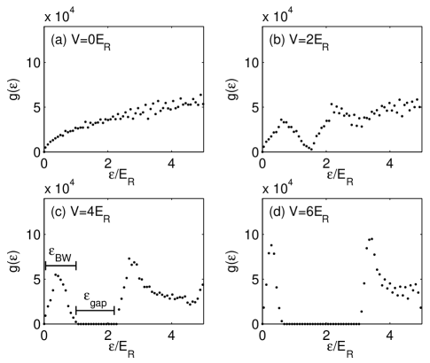
Figure 1: Density of states for a $N_{s}\approx 3\times 10^{4}$ site cubic lattice at various depths. For a depth of approximately $V=2E_{R}$ a gap develops in the density of states. In (c) we illustrate the energy gap, $\epsilon_{{\rm gap}}$, and ground bandwidth, $\epsilon_{{\rm BW}}$. Points are determined by numerically averaging the exact spectrum over a small energy range.

In general we note that the lattice leads to a substantial change in the the density of states, $g(\epsilon)$, for the system. In the absence of the lattice (Fig. 1(a)) the density of states is that for free particles in a box, and is proportional to $\sqrt{\epsilon}$. The smoothness of $g(\epsilon)$ is disrupted by the presence of a lattice, which causes flat regions in the energy bands giving rise to peaked features in the density of states, known as van Hove singularities Ashcroft and Mermin (1976). The van Hove singularities in the first and second energy bands are clearly visible in Figs. 1(b)-(d). For sufficiently deep lattices an energy gap, $\epsilon_{{\rm gap}}$, will separate the ground and first excited bands. For the cubic lattice we consider here, a finite gap appears at a lattice depth of $V\approx 2E_{R}$ (see Fig. 1(b)), and beyond this depth the gap increases with lattice depth (see Figs. 1(c)-(d)). In forming the gap higher energy bands are shifted up-wards in energy, and the ground band becomes compressed — a feature characteristic of the reduced tunneling between lattice sites. We refer to the energy range over which the ground band extends as the (ground) band width, $\epsilon_{{\rm BW}}$. This quantity decreases in magnitude exponentially with $V$ (see Figs.1(b)-(c)), causing the ground band to have an extremely high density of states for deep lattices; generally in this limit quantum many-body effects will significantly modify the energy spectra of the lowest band from the non-interacting states we use here. We will discuss the effects of interactions in Sec. III.4.

III Results

Figure 2: Entropy versus temperature curves for a $N_{s}\approx 3\times 10^{4}$ site cubic lattice, with filling factor $n=0.25$ at various depths $V=0$ to $20E_{R}$ (with a spacing of $2E_{R}$ between each curve). The entropy plateau $S_{0}$ is shown as a dashed line and the condensation point is marked on each curve as a circle. Dotted line marked $A$ shows a path along which adiabatic loading into the lattice causes the temperature to increase. Dotted line marked $B$ shows a path along which adiabatic loading into the lattice causes the temperature to decrease.

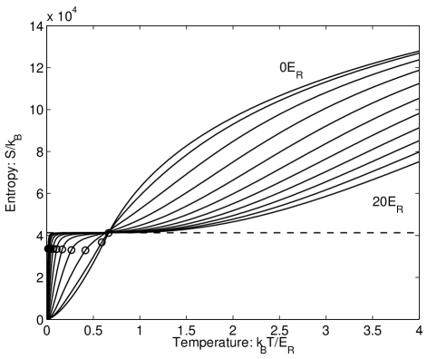
Figure 3: Entropy versus temperature curves for a $N_{s}\approx 3\times 10^{4}$ site cubic lattice, with filling factor $n=1$ at various depths$V=0$ to $20E_{R}$ (with a spacing of $2E_{R}$ between each curve). The entropy plateau $S_{0}$ is shown as a dashed line and the condensation point is marked on each curve as a circle.

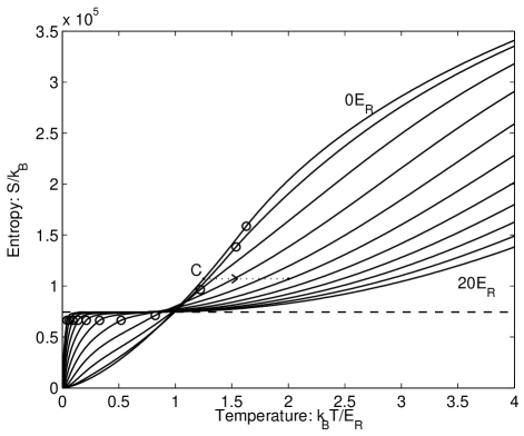
Figure 4: Entropy versus temperature curves for a $N_{s}\approx 3\times 10^{4}$ site cubic lattice, with filling factor $n=4$ at various depths $V=0$ to $20E_{R}$ (with a spacing of $2E_{R}$ between each curve). The entropy plateau $S_{0}$ is shown as a dashed line and the condensation point is marked on each curve as a circle. Dotted line marked $C$ shows a path along which an initially Bose-condensed system uncondenses as it is loaded into the lattice at $V\approx 4E_{R}$.

In Figs. 2-4 we show entropy-temperature curves for various lattice depths and filling factors $n$. These curves have been calculated for a lattice with $31$ lattice sites along each spatial dimension, i.e. $N_{s}\approx 3\times 10^{4}$. The condensation temperature is defined as that at which 1% of all particle occupy the ground state, and is indicated in Figs. 2-4. We note that being a finite system the transition is not discontinuous, however the onset of condensation is rapid and changing the requirement to 5% makes little observable difference in the critical point locations.

An important common feature to these curves is the distinct separation of regions where adiabatic loading causes the temperature of the sample to increase or decrease, which we will refer to as the regions of heating and cooling respectively. These two regions are separated by a common point that all curves approximately pass through, and we denote by its coordinates as $\{T_{0},S_{0}\}$. The reason for the existence of this point will be discussed below. For cases considered in Figs. 2-4 $T_{0}$ is in the range $0.5-1E_{R}$, and to clearly indicate the vertical separation of the heating and cooling regions, we have marked $S_{0}$ as a horizontal dashed line.

We now explicitly demonstrate the temperature changes that occur during adiabatic loading using two possible adiabatic processes labeled $A$ and $B$, and marked as dotted lines in Fig. 2. Process $A$ begins with a gas of free particles in an initial state with $S>S_{0},$ $T>T_{0}$. As the gas is loaded into the lattice the process line indicates that the temperature increases rapidly with the lattice depth. Conversely process $B$ begins with a gas of free particles in an initial state with $S<S_{0},$ $T<T_{0},$ and the lattice loading causes a rapid decrease in temperature. This behavior can be qualitatively understood in terms of the modifications the lattice makes to the energy states of the system. As is apparent in Fig. 1, the ground band flattens for increasing lattice depth causing the density of states to be more densely compressed at lower energies. Thus in the lattice all these states can be occupied at a much lower temperature than for the free particle case. As we discuss below, $S_{0}$ is the maximum entropy available from only accessing states of the lowest band, and so for $S>S_{0}$ higher bands are important. As the lattice depth and hence $\epsilon_{{\rm gap}}$ increases, the temperature must increase for these excited states to remain accessible.

III.1 Entropy plateau

In Figs. 2-4 a horizontal plateau (at the level marked by the dashed lines) is common to the entropy-temperature curves for larger lattice depths ($V\gtrsim 8E_{R}$). This occurs because for these lattices $\epsilon_{{\rm BW}}\ll\epsilon_{{\rm gap}}$, and there is a large temperature range over which states in the excited bands are unaccessible, yet all the ground band states are uniformly occupied. The entropy value indicated by the dashed line in Figs. 2-4 corresponds to the total number of $N_{p}$-particle states in the ground band. Since the number of single particle energy states in the ground band is equal to the number of lattice sites, the total number of available $N_{p}$-particle states, which we define as $\Omega_{0}$, is the number of distinct ways $N_{p}$ identical bosons can be placed into $N_{s}$ states, i.e.

$$\Omega_{0}=\frac{(N_{p}+N_{s}-1)!}{N_{p}!(N_{s}-1)!}.$$ (6)

The associated entropy $S_{0}=k_{B}\log\Omega_{0}$, which we shall refer to as the plateau entropy, can be evaluated using Sterling’s approximation

$$S_{0} \simeq k_{B}\Big{[}N_{p}\log\left(\frac{N_{p}+N_{s}-1}{N_{p}}\right)$$

$$+(N_{s}-1)\log\left(\frac{N_{p}+N_{s}-1}{N_{s}-1}\right)\Big{]}.$$

As described earlier, this entropy value separates the heating and cooling regions for the lattice.

III.2 Scaling

Here we give limiting results for the entropy-temperature curves.

III.2.1 $k_{B}T\ll\epsilon_{{\rm BW}}.$

When the temperature is small compared to the ground band width, only energy states near the ground state of the lowest band are accessible to the system. These states exhibit a quadratic dependence on the magnitude of the quasimomentum and the entropy of this system is well described by the free particle expression if the bare particle mass is replaced by the effective mass i.e. $m\to m^{*}$. In general this regime occurs only at very low temperatures, and except for extremely low filling factors the system will be condensed in this region. In this limit the expression for entropy corresponds to the expression for a condensed gas of free particles with mass $m^{*}$

$$S=\frac{5}{2}N_{s}a^{3}\zeta(5/2)\left(\frac{m^{*}k_{B}T}{2\pi\hbar^{2}}\right)^{\frac{3}{2}},$$ (8)

where $\zeta(n)=\sum_{k=1}^{\infty}1/k^{n}$ is the Riemann Zeta function and $N_{s}a^{3}$ is the volume of the system Pethick and Smith (2002). We note that in this regime the critical temperature for condensation scales as $T_{c}\sim(m^{*})^{-3/2}$, so that $T/T_{c}$ is independent of $m^{*}$ and hence the lattice depth.

III.2.2 Tight-binding limit with $k_{B}T\ll\epsilon_{{\rm gap}}$

As discussed in Sec. III.1, when the temperature is small compared to the energy gap only states within the ground band are accessible to the system. In addition when the tight-binding description is applicable for the initial and final states of an adiabatic process, the initial and final properties are related by a scaling transformation.

To illustrate we consider our initial system to be in equilibrium with entropy $S_{i}<S_{0}$, in lattice of depth $V_{i}$ which we take to be sufficiently deep enough for tight-binding expression (3) to be a good description of the ground band energy states. If an adiabatic process is used to take the system to some final state at lattice depth $V_{f}$ (also in the tight-binding regime) it is easily shown that the macroscopic parameters of the initial and final states are related as

$$E_{f} = \alpha E_{i},$$ (9)

$$T_{f} = \alpha T_{i},$$ (10)

$$\mu_{f} = \alpha\mu_{i},$$ (11)

where the scale factor

$$\alpha=m_{i}^{*}/m_{f}^{*}$$ (12)

is the ratio of the effective masses, and the subscripts $i$ and $f$ refer to quantities associated with the initial and final states respectively. This type of scaling relation leaves the occupations of the single particle levels (including the condensate occupation) unchanged. This means that being adiabatic does not require redistribution through collisions and may allow the lattice depth to be changed more rapidly. However, adiabaticity with respect to the many-body wavefunction will become a significant constraint as the lattice depth increases and will become the limiting timescale.

III.3 Condensation

The temperature and entropy at which bosons condense generally changes with lattice depth as indicated in Figs. 2-4. We note that for high filling factors the condensation points for different lattice depths occur over a wide range of entropies, suggesting that the degree of condensation will be greatly affected by adiabatic lattice loading.

For instance, consider the adiabatic process indicated by the dotted line and labeled $C$ in Fig. 4. The system starts as a Bose-condensed gas of free particles. However, as the lattice depth increases the condensate fraction decreases until the system passes through the transition point and becomes uncondensed. This process is reversible, and is analogous to the experiments by Stamper-Kurn et al. Stamper-Kurn et al. (1998), where a Bose gas was reversibly condensed by changing the shape of the trapping potential.

We note that the free particle case with $n=1$ shown in Fig. 3 condenses at an entropy approximately equal to the plateau entropy $S_{0}$, given by Eq. (III.1). For an ideal gas of free particles condensation occurs when the entropy of the system is $S_{{\rm cond}}=\frac{5}{2}k_{B}N_{p}\zeta(\frac{5}{2})/\zeta(\frac{3}{2}),$ (e.g. see Pethick and Smith (2002)), whereas the plateau entropy for a lattice with unit filling is $S_{0}(n\!=\!1)=2k_{B}N_{p}\log(2)$, (obtained by setting $(N_{s}-1)\to N_{s}$ and $N_{p}=N_{s}$ in Eq. (III.1)). In comparing the values we find $S_{0}(n\!=\!1)/S_{{\rm cond}}\approx 1.0798$, in agreement with numerical observation. For fixed $N_{s}$ the filling factor is proportional to $N_{p}$, thus the free particle condensation entropy scales as $S_{{\rm cond}}\sim n$ whereas the entropy plateau goes as $S_{0}\sim\log(n)$. So we conclude that for $n\gtrsim 1$ condensation occurs (for free particles) above the plateau, whereas for $n\lesssim 1$ it occurs below the plateau.

III.4 Interaction effects

We now turn to a qualitative discussion of interaction effects on the system. To do this we employ Bogoliubov’s method for treating an interacting Bose gas. In this approach all the atoms are assumed to be in the zero quasi-momentum condensate, and by diagonalizing an approximation to the many-body Hamiltonian a set of quasiparticle levels are obtained (e.g. see Berg-Sørensen and Mølmer (1998); Burnett et al. (2002)). This approach should be a good approximation to the exact many-body spectrum for moderate lattice depths (i.e. below the depth where the Mott-transition occurs) and small thermal depletion.

The regimes of cooling associated with lattice loading observed in Figs. 2-4 arose from the rapid compression of the ground band width ($\epsilon_{{\rm BW}}$) that occurs with increasing lattice depth. To assess the effects of interactions on cooling we compare the width of the ground band calculated with Bogoliubov theory to the non-interacting case for parameters relevant to current experiments in Fig. 5(a). These results demonstrate that interactions suppress the rate at which the bandwidth decreases as the lattice is applied. We also note that the band gap is modified by interactions, however the thermodynamic properties of the system are not as sensitive to small changes in this and we will not consider the effect of this.

To quantify how the modified ground band excitation spectrum affects thermodynamic properties of the system we consider an extension of the arguments made in Sec. III.2.2. In that section we discussed the scaling relationship that could be applied to the thermodynamic quantities for a Bose gas in the tight-binding regime when only states of the ground band were relevant. For the interacting case we can apply the same argument if we ignore any ground band spectrum reshaping with varying lattice depth, other than a scale change given by the scaling parameter $\alpha=(\epsilon_{{\rm BW}})_{f}/(\epsilon_{{\rm BW}})_{i}$, where $(\epsilon_{{\rm BW}})_{i}$ and $(\epsilon_{{\rm BW}})_{f}$ are the respective bandwidths of the initial and final configurations (both assumed to be in the tightbinding limit). We note that this definition of $\alpha$ is equivalent to Eq. (12) for the non-interacting case. As was shown in Eq. (10), the ratio of final to initial temperatures is equal to $\alpha.$ In Fig. 5(b) we compare the values of $\alpha$ both with and without interactions for a system initially in a $V=4E_{R}$ deep lattice, for various final depths $V$ . These results quantify how interactions lead to a lesser degree of cooling, and (in the limit of the Bogoliubov approach) these results suggest that the temperature will level out to some finite non-zero value at large lattice depths.

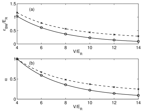
Figure 5: Bogoliubov description of interaction effects on the (a) bandwidth and (b) scaling parameter $\alpha$ for various lattice depths. Crosses: interacting result for $n=1$. Circles: non-interacting result. Other parameters: $\lambda=850$nm and collisional interaction strength taken for Rb⁸⁷.

In the Mott-insulator regime (where Bogoliubov approach is invalid) an energy gap proportional to the on-site interaction strength develops between the ground state and the particle-hole excitations above it (see Jaksch et al. (1998)). This suggests that in general interactions tend to increase ground band width, and will limit our ability to cool the system with adiabatic passage.

III.5 Adiabaticity

Finally we note that interactions between particles are essential for establishing equilibrium in the system, and understanding this in detail will be necessary to determine the timescale for adiabatic loading. In general this requirement is difficult to assess, and in systems where there is an additional external potential it seems that the adiabaticity requirements will likely be dominated by the process of atom transport within the lattice to keep the chemical potential uniform, though recent proposals have suggested ways of reducing this problem Sklarz et al. (2002).

It seems reasonable that for sufficiently deep lattices the decreasing tunneling rate will ultimately become the rate limiting timescale for maintaining adiabaticity in adiabatic loading (e.g. see Band and Trippenbach (2002)). To estimate this timescale we consider a case relevant to ⁸⁷Rb experiments. For a lattice depth of a $V=10E_{R}$, where we have taken $\lambda=850$nm, the tunneling time is $\sim 10$ms. This timescale is short compared to the loading time used in recent experiments with this system Orzel et al. (2001); Greiner et al. (2002b), and suggests that smoothly increasing the lattice to depths of $\sim 10E_{R}$ over $>100$ms should be very adiabatic. For depths larger that $V=10E_{R}$ the tunneling time increases exponentially and the adiabatic condition becomes more difficult to satisfy, however this is also the regime where many-body effects will begin to dominate and a more complete description will be needed to fully understand the adiabaticity requirements.

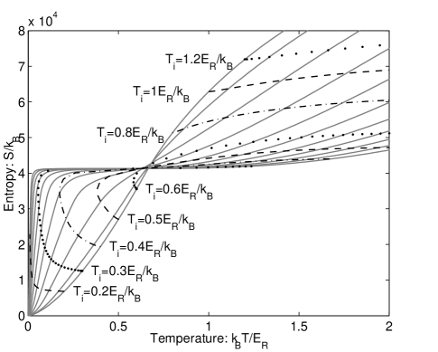
Figure 6: Fast lattice loading of a $N_{s}\approx 3\times 10^{4}$ site cubic lattice, with filling factor $n=1$. Broken/dotted/dashed lines indicate fast loading curves (see text) and are labeled by the temperature of the initial $V=0$ state. The lattice depth on these curves can be determined from their intercept with the equilibrium entropy versus temperature curves (gray solid lines), which are described in Fig. 3.

It is useful to assess the degree to which non-adiabatic loading would cause heating in the system. We consider lattice loading on a time scale fast compared to the typical collision time between atoms, yet slow enough to be quantum mechanically adiabatic with respect to the single particle states. This latter requirement excludes changing the lattice so fast that band excitations are induced, and it has been shown that in practice this condition can be satisfied on very short time scales Denschlag et al. (2002). We will refer to this type of loading as fast lattice loading, to distinguish it from the fully adiabatic loading we have been considering thus far.

To simulate the fast lattice loading we take the system to be initially in equilibrium at temperature $T_{i}$ for zero lattice depth. For the final lattice depth we fast load into, we map the initial single particle distribution onto their equivalent states in the final lattice, and calculate the total energy for this final non-equilibrium configuration. This procedure assumes that there has been no collisional redistribution to allow the system to adjust to the changing potential. To determine the thermodynamic state the final distribution will relax to, we use the energy of the non-equilibrium distribution as a constraint for finding the equilibrium values of temperature and entropy. In general the final state properties will depend on the initial temperature, filling factor, and final depth of the lattice, and to illustrate typical behavior we show a set of fast loading process curves that indicate the final state equilibrium properties as a function of final lattice depth in Fig. 6 for unit filling and various initial temperatures.

These curves show, as is expected from standard thermodynamic arguments, that entropy always increases for non-adiabatic processes, i.e. all loading curves in Fig. 6 bend up wards with increasing lattice depth. We also observe that eventually all curves predict heating for large enough final lattice depth. However, for initial temperatures sufficiently far below the critical temperature for cooling $(T_{0}\sim 0.7E_{R}/k_{B}$) a useful degree of temperature reduction can be achieved with fast lattice loading up to certain maximum depth. For example, the curve with initial temperature $T_{i}=0.5E_{R}/k_{B}$ in Fig. 6 cools for final depths less than $V\sim 5E_{R}$, but for depths greater than this the temperature begins to increase quite rapidly.

IV 2D Lattice with dipole confinement

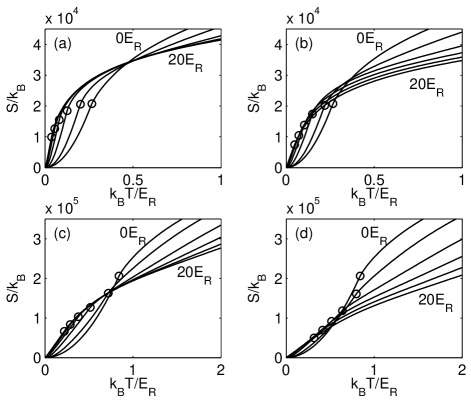
Figure 7: Entropy versus temperature curves for a $N_{s}\approx 10^{2}$ site 2D square lattice with harmonic trapping potential in the perpendicular direction, for various lattice depths and strengths of harmonic confinement. Results are given 2D site occupations of (a)-(b) $n=10$, and (c)-(d) $n=100$. In each subplot the various curves correspond to lattices depths of $V=0$ to $20E_{R}$ (with a spacing of $4E$ between each curve). In (a) and (c) the harmonic confinement frequency is $f_{T}=0.01E_{R}/h$, whereas in (b) and (d) $f_{T}=0.01E_{R}/h$ at $V=0$, and is taken to increase by $2\times 10^{-3}E_{R}$ for each subsequent lattice depth, to $f_{T}=0.02E_{R}$ at $V=20E_{R}$. The condensation point for the system is marked with a circle on each curve.

Here we consider the case of a 2D lattice in the $xy$-plane with a harmonic trapping potential along the $z$ direction. We calculate the eigenstates of the Schrödinger equation with potential energy

$$V_{T}(\mathbf{r})=\frac{V}{2}[\cos(2kx)+\cos(2ky)]+\frac{1}{2}m(2\pi f_{T})^{2}z^{2},$$

where $f_{T}$ is the harmonic trap frequency. In Fig. 7 we give the entropy versus temperature curves for a range of experimentally relevant parameters. The results in Figs. 7 (a) and (c) demonstrate the behavior for a range of lattice depths and two different atom densities, but with constant harmonic trap frequency. These curves exhibit qualitative similarities with the 3D lattice curves shown in Figs. 2-4, such as a crossing region where the zero-depth curve changes from being a lower bound to an upper bound of the other curves, and separates the regions where adiabatic loading of the system will cool or heat the system respectively. Similar to the 3D case, this behavior arises because of how the lattice modifies the energy spectrum, i.e. the compression of low lying states and upward shift of high lying states. However, the availability of equally spaced harmonic oscillator states ensures that the density of states does not have a gap (assuming $f_{T}$ is small compared to $V$) and an entropy plateau does not appear. We note that the condensation temperature decreases more rapidly both with temperature and entropy compared to the 3D cases, making the 2D lattice a more ideal system for observing reversible condensation.

In Figs. 7 (b) and (d) we consider equivalent systems to those in Figs. 7 (a) and (c), except that we increase the trap frequency with lattice depth to model the effects of additional dipole confinement on the system. For the case of rubidium and taking $\lambda\sim 805$nm, these results correspond to a harmonic confinement of $f_{T}\sim 35$Hz at zero lattice depth, with the confinement increasing in linear steps on successive curves up to a maximum value $f_{T}\sim 70$Hz at $V=20E_{R}$, typical of current experimental parameters. These results demonstrate that the additional dipole confinement reduces the size of the region over which cooling occurs, and reduces the extend to which the system can be cooled. The more rapidly $f_{T}$ increases with lattice depth, the more pronounced this reduction will be.

V Conclusion

In this paper we have calculated the entropy-temperature curves for bosons in a 3D optical lattice, and a 2D lattice with harmonic confinement for various depths and filling factors. We have identified general features of the thermodynamic properties relevant to lattice loading, indicated regimes where adiabatically changing the lattice depth will cause heating or cooling of the atomic sample, and have provided limiting results for the behavior of the entropy curves. We have considered the effect of lattice depth and filling factor on the Bose condensation point and have examined the possibility of reversible condensation through lattice loading. We have discussed the dominant effects of interactions, and have shown that many of our predictions are robust to non-adiabatic effects. Future extensions to this work will consider in more detail the effects of both interactions and inhomogeneous external potentials.

References

- Orzel et al. (2001) C. Orzel, A. K. Tuchman, M. L. Fenselau, M. Yasuda, and M. A. Kasevich, Science 23, 2386 (2001).
- Greiner et al. (2002a) M. Greiner, O. Mandel, T. W. Hänsch, and I. Bloch, Nature 419, 51 (2002a).
- Greiner et al. (2002b) M. Greiner, O. Mandel, T. Esslinger, T. W. Hänsch, and I. Bloch, Nature 415, 39 (2002b).
- (4) O. Mandel, M. Greiner, A. Widera, T. Rom, T. Hänsch, and I. Bloch, Coherent transport of neutral atoms in spin-dependent optical lattice potentials, cond-mat/0301169.
- Calarco et al. (2000) T. Calarco, H. Briegel, D. Jaksch, J. I. Cirac, and P. Zoller, J. of Mod. Opt. 47, 2137 (2000).
- Deutsch et al. (2000) I. H. Deutsch, G. K. Brennen, and P. S. Jessen, Forschritte der Physik 48, 925 (2000).
- Burger et al. (2002) S. Burger, F. S. Cataliotti, C. Fort, P. Maddaloni, F. Minardi, and M. Inguscio, Europhys. Latt. 57, 1 (2002).
- Olshanii and Weiss (2002) M. Olshanii and D. Weiss, Phys. Rev. Lett. 89, 090404 (2002).
- Ashcroft and Mermin (1976) N. W. Ashcroft and N. D. Mermin, Solid State Physics (W.B. Saunders Company, 1976).
- Pethick and Smith (2002) C. Pethick and H. Smith, Bose-Einstein condensation in dilute gases (Cambridge University Press, 2002).
- Stamper-Kurn et al. (1998) D. Stamper-Kurn, H.-J. Miesner, A. Chikkatur, S. Inouye, J. Stenger, and W. Ketterle, Phys. Rev. Lett. 81, 2194 (1998).
- Berg-Sørensen and Mølmer (1998) K. Berg-Sørensen and K. Mølmer, Phys. Rev. A 58, 1480 (1998).
- Burnett et al. (2002) K. Burnett, M. Edwards, C. W. Clark, and M. Shotter, J. Phys. B 35, 1671 (2002).
- Jaksch et al. (1998) D. Jaksch, C. Bruder, J. I. Cirac, C. Gardiner, and P. Zoller, Phys. Rev. Lett. 81, 3108 (1998).
- Sklarz et al. (2002) S. E. Sklarz, I. Friedler, D. J. Tannor, Y. B. Band, and C. J. Williams, Phys. Rev. A 66, 053620 (2002).
- Band and Trippenbach (2002) Y. B. Band and M. Trippenbach, Phys. Rev. A 65, 053602 (2002).
- Denschlag et al. (2002) J. H. Denschlag, J. E. Simsarian, H. Häffner, C. McKenzie, A. Browaeys, D. Cho, K. Helmerson, S. L. Rolston, and W. D. Phillips, J. Phys. B 35, 3095 (2002).