Finite temperature excitations of a trapped Bose-Fermi mixture

Abstract

We present a detailed study of the low-lying collective excitations of a spherically trapped Bose-Fermi mixture at finite temperature in the collisionless regime. The excitation frequencies of the condensate are calculated self-consistently using the static Hartree-Fock-Bogoliubov theory within the Popov approximation. The frequency shifts and damping rates due to the coupled dynamics of the condensate, noncondensate, and degenerate Fermi gas are also taken into account by means of the random phase approximation and linear response theory. In our treatment, the dipole excitation remains close to the bare trapping frequency for all temperatures considered, and thus is consistent with the generalized Kohn theorem. We discuss in some detail the behavior of monopole and quadrupole excitations as a function of the Bose-Fermi coupling. At nonzero temperatures we find that, as the mixture moves towards spatial separation with increasing Bose-Fermi coupling, the damping rate of the monopole (quadrupole) excitation increases (decreases). This provides us a useful signature to identify the phase transition of spatial separation.

I introduction

The impressive experimental achievement of Bose-Einstein condensation (BEC) in the bosonic systems ⁸⁷Rb jila , ²³Na mit , and ⁷Li rice has initiated and stimulated a whole new field of research in the physics of quantum atomic gases. Recently, several groups have extended these experiments to the case of trapped Bose-Fermi mixtures, in order to employ the “sympathetic cooling” to reach the regime of quantum degeneracy for the Fermi gas. As a first step, stable Bose-Einstein condensates immersed in a degenerate Fermi gas have been realized with ⁷Li in ⁶Li lili , ²³Na in ⁶Li nali , and very recently with ⁸⁷Rb in ⁴⁰K lens . In the possible next step, investigations of the thermodynamics, collective many-body effects and other properties could be available soon in these systems. Especially interesting is the behavior of low-energy collective excitations, since the high accuracy of frequency measurements and the sensitivity of collective phenomena to the interatomic interaction make them good candidates to unravel the dynamical correlation of the many-body system.

On the theoretical side, several analyses have been presented for low-lying collective excitations of a trapped Bose-Fermi mixture. Collective modes in the collisionless limit, where the collision rate is small compared with the frequencies of particle motion in traps, have been considered by the sum-rule approach sumrules , by the scaling theory liu , or in the random-phase approximation capuzzi ; rpa . In the collision-dominated regime collective oscillations have been discussed by Tosi et al. in Refs. tosi00 ; tosi03 , and by the authors in Ref. liu . These investigations have mainly concentrated at zero temperature using the standard two-fluid model for the condensate and the degenerate Fermi gas. However, the realistic experiment is most likely carried out at relatively higher temperatures, where the condensate oscillates in the presence of a considerably large fraction of above-condensate atoms. It thus seems timely to develop an extension of these theories to the finite temperature.

In the present paper we investigate the low-lying collective excitations of a spherically trapped Bose-Fermi mixture at finite temperature in the collisionless regime. We confine ourselves to the collective modes of the condensate, i.e., the density oscillations of the condensate. We first calculate the mode frequencies by using the simplest temperature-dependent mean-field theory — the Popov version of the Hartree-Fock-Bogoliubov (HFB) theory — that has been generalized by us to a trapped Bose-Fermi mixture to study its thermodynamics hu . For a purely Bose gas, it is well known that the HFB-Popov theory includes only the static mean-field effects of the noncondensate atoms griffin and thus predicts the correct mode frequency only at temperatures $T\lesssim T_{0}=0.65T_{c}$ burnett , where $T_{c}$ is the critical temperature of BEC. Above $T_{0}$ the noncondensate component becomes considerably large and its dynamics should be treated on an equal footing with that of the condensate giorgini ; stoof ; zgn ; fedichev ; reidl . In our case of Bose-Fermi mixtures, the situation is more crucial. Due to the large number of fermions, the coupled dynamics of the condensate, noncondensate, and degenerate Fermi gas has to be taken into account even at zero temperature. In this paper, we shall treat it perturbatively in the spirit of the random phase approximation (RPA) and linear response theory. We derive the explicit expression for the frequency shift and damping rate arising from the coupled dynamics, which in the absence of the Bose-Fermi interaction coincides with the finding of Ref. giorgini . Based on this expression and the static HFB-Popov theory, we present a detailed numerical study of the monopole and quadrupole condensate oscillations against the Bose-Fermi coupling. The dipole excitation is also studied and found to be consistent with the generalized Kohn theorem.

The paper is organized as follows. In the next section we derive the theory used in this paper. In Sec. III we apply this theory to mixtures of ${}^{41}{\rm K}-^{40}$K and ${}^{87}{\rm Rb}-^{40}$K, and calculate the dispersion relation of the monopole and quadrupole excitations as a function of the Bose-Fermi coupling. The behavior of monopole and quadrupole modes against temperature is also discussed in detail. Finally, section IV is devoted to conclusions.

II formulation

In this section we first generalize a time-dependent mean-field scheme developed by Giorgini giorgini to Bose-Fermi mixtures, and derive the equation for the small-amplitude oscillations of the condensate. Since the formalism of this time-dependent mean-field approximation for an inhomogeneous interacting Bose gas has already been presented in detail in Ref. giorgini , here we shall merely concentrate on the key points, and indicate the necessary modification in the presence of the fermionic component. By means of the RPA and linear response theory, we further consider the fluctuations of the noncondensate and of the degenerate Fermi gas induced by the condensate oscillations. The back action of these fluctuations on the condensate motion is then calculated perturbatively to second order in the interaction coupling constant to obtain the explicit expression for frequency shifts and damping rates.

Our starting point is the trapped binary Bose-Fermi mixture that is portrayed as a thermodynamic equilibrium system under the grand canonical ensemble whose thermodynamic variables are $N_{b}$ and $N_{f}$, respectively, the total number of trapped bosonic and fermionic atoms, $T$, the absolute temperature, and $\mu_{b}$ and $\mu_{f}$, the chemical potentials. In terms of the creation and annihilation bosonic (fermionic) field operators $\psi^{+}({\bf r},t)$ and $\psi({\bf r},t)$ ($\phi^{+}({\bf r},t)$ and $\phi({\bf r},t)$), the density Hamiltonian of the system takes the form (in units of $\hbar=1$, and all field operators depend on ${\bf r}$ and $t$)

$${\cal H} = {\cal H}_{b}+{\cal H}_{f}+{\cal H}_{bf},$$

$${\cal H}_{b} = \psi^{+}\left[-\frac{{\bf\bigtriangledown}^{2}}{2m_{b}}+V_{trap}^{b}({\bf r})-\mu_{b}\right]\psi+\frac{g_{bb}}{2}\psi^{+}\psi^{+}\psi\psi,$$

$${\cal H}_{f} = \phi^{+}\left[-\frac{{\bf\bigtriangledown}^{2}}{2m_{f}}+V_{trap}^{f}({\bf r})-\mu_{f}\right]\phi,$$

$${\cal H}_{bf} = g_{bf}\psi^{+}\psi\phi^{+}\phi.$$ (1)

Here we consider a spherically symmetric system, with static external potentials $V_{trap}^{b,f}({\bf r})=m_{b,f}\omega_{b,f}^{2}r^{2}/2$, where $m_{b,f}$ are the atomic masses, and $\omega_{b,f}$ are the trap frequencies. The interaction between bosons and between bosons and fermions are described by the contact potentials and are parameterized by the coupling constants $g_{bb}=4\pi\hbar^{2}a_{bb}/m_{b}$ and $g_{bf}=2\pi\hbar^{2}a_{bf}/m_{r}$, to the lowest order in the $s$-wave scattering length $a_{bb}$ and $a_{bf}$, with $m_{r}=m_{b}m_{f}/(m_{b}+m_{f})$ being the reduced mass.

II.1 time-dependent mean-field approximation

According to the usual treatment for Bose system with broken gauge symmetry, we shall apply the decomposition: $\psi({\bf r},t)=\Phi({\bf r},t)+\tilde{\psi}({\bf r},t),$ where $\Phi({\bf r},t)\equiv\left\langle\psi({\bf r},t)\right\rangle$ represents a time-dependent condensate wave function and allows us to describe situations in which the system is displaced from equilibrium and the condensate is oscillating in time. With this respect the average $\left\langle...\right\rangle$ is intended to be a non-equilibrium average, while time-independent equilibrium averages will be indicated in this paper with the symbol $\left\langle...\right\rangle_{0}$. The field operator $\tilde{\psi}({\bf r},t)$ plays the role of excitations out of the condensate, and by definition satisfies the condition $\left\langle\tilde{\psi}({\bf r},t)\right\rangle=0$. This ansatz is then inserted in the equation of motion for $\psi({\bf r},t)$:

$$i\frac{\partial}{\partial t}\psi = \left[-\frac{{\bf\bigtriangledown}^{2}}{2m_{b}}+V_{trap}^{b}({\bf r})-\mu_{b}\right]\psi$$ (2)

$$+g_{bb}\psi^{+}\psi\psi+g_{bf}\psi\phi^{+}\phi.$$

Taking a statistical average over Eq. (2) and setting the triplet average values $\left\langle\tilde{\psi}^{+}({\bf r},t)\tilde{\psi}({\bf r},t)\tilde{\psi}({\bf r},t)\right\rangle$ and $\left\langle\tilde{\psi}({\bf r},t)\phi^{+}({\bf r},t)\phi({\bf r},t)\right\rangle$ to zero note thus leads to the following equation of motion for the condensate wave function

$$i\frac{\partial}{\partial t}\Phi({\bf r},t) = \left[-\frac{{\bf\bigtriangledown}^{2}}{2m_{b}}+V_{trap}^{b}({\bf r})-\mu_{b}\right]\Phi({\bf r},t)$$ (3)

$$+g_{bb}\left|\Phi({\bf r},t)\right|^{2}\Phi({\bf r},t)+2g_{bb}\tilde{n}({\bf r},t)\Phi({\bf r},t)$$

$$+g_{bb}\tilde{m}({\bf r},t)\Phi^{*}({\bf r},t)+g_{bf}n_{f}({\bf r},t)\Phi({\bf r},t),$$

where the densities are defined, respectively, as $\tilde{n}({\bf r},t)\equiv\left\langle\tilde{\psi}^{+}({\bf r},t)\tilde{\psi}({\bf r},t)\right\rangle$, $\tilde{m}({\bf r},t)\equiv\left\langle\tilde{\psi}({\bf r},t)\tilde{\psi}({\bf r},t)\right\rangle,$ and $n_{f}({\bf r},t)\equiv\left\langle\phi^{+}({\bf r},t)\phi({\bf r},t)\right\rangle$. Under the stationary condition, we replace $\Phi({\bf r},t)$, $\tilde{n}({\bf r},t)$, $\tilde{m}({\bf r},t)$ and $n_{f}({\bf r},t)$ by their equilibrium values $\Phi_{0}({\bf r})\equiv\left\langle\psi({\bf r})\right\rangle_{0}$, $\tilde{n}^{0}({\bf r})\equiv\left\langle\tilde{\psi}^{+}({\bf r})\tilde{\psi}({\bf r})\right\rangle_{0}$, $\tilde{m}^{0}({\bf r})\equiv\left\langle\tilde{\psi}({\bf r})\tilde{\psi}({\bf r})\right\rangle_{0}$ and $n_{f}^{0}({\bf r})\equiv\left\langle\phi^{+}({\bf r})\phi({\bf r})\right\rangle_{0}$, respectively. This yields the generalized time-independent Gross-Pitaevskii (GP) equation for Bose-Fermi mixtures hu

$$\left[-\frac{{\bf\bigtriangledown}^{2}}{2m_{b}}+V_{trap}^{b}-\mu_{b}+g_{bb}\left(n_{0}+2\tilde{n}^{0}\right)+g_{bf}n_{f}^{0}\right]\Phi_{0}=0,$$ (4)

where $n_{0}({\bf r})=\left|\Phi_{0}({\bf r})\right|^{2}$ is the condensate density. In the above equation, we already use the Popov prescription: $\tilde{m}^{0}({\bf r})=0,$ which amounts to neglect the effects arising from the equilibrium anomalous density note2 .

We are interested in the small amplitude oscillations of the condensate, which is only slightly displaced from its stationary value $\Phi_{0}({\bf r})$: $\Phi({\bf r},t)=\Phi_{0}({\bf r})+\delta\Phi({\bf r},t),$ where $\delta\Phi({\bf r},t)$ is a small fluctuation. This small oscillations can consequently induce small fluctuations of the densities around their equilibrium values: $\tilde{n}({\bf r},t)=\tilde{n}^{0}({\bf r})+\delta\tilde{n}({\bf r},t)$, $\tilde{m}({\bf r},t)=\delta\tilde{m}({\bf r},t)$, and $n_{f}({\bf r},t)=n_{f}^{0}({\bf r})+\delta n_{f}({\bf r},t)$. The time-dependent equation for $\delta\Phi({\bf r},t)$ is then obtained by linearizing the equation of motion (3)

$$i\frac{\partial}{\partial t}\delta\Phi({\bf r},t) = {\cal L}\delta\Phi({\bf r},t)+g_{bb}n_{0}({\bf r})\delta\Phi^{*}({\bf r},t)$$ (5)

$$+2g_{bb}\Phi_{0}({\bf r})\delta\tilde{n}({\bf r},t)+g_{bb}\Phi_{0}({\bf r})\delta\tilde{m}({\bf r},t)$$

$$+g_{bf}\Phi_{0}({\bf r})\delta n_{f}({\bf r},t),$$

where we have introduced the Hermitian operator

$${\cal L\equiv}-\frac{{\bf\bigtriangledown}^{2}}{2m_{b}}+V_{trap}^{b}\left({\bf r}\right)-\mu_{b}+2g_{bb}n_{b}^{0}({\bf r})+g_{bf}n_{f}^{0}({\bf r}),$$ (6)

and $n_{b}^{0}({\bf r})=n_{0}({\bf r})+\tilde{n}^{0}({\bf r})$, the total density of bosons. In Eq. (5), the terms containing $\delta\tilde{n}$, $\delta\tilde{m}$ and $\delta n_{f}$ account for the dynamic coupling between the condensate and the fluctuations of the noncondensate component and of the degenerate Fermi gas. Assuming that the condensate oscillates with frequency $\omega$: $\delta\Phi({\bf r},t)=\delta\Phi({\bf r})e^{-i\omega t}$ and $\delta\Phi^{*}({\bf r},t)=\delta\Phi^{*}({\bf r})e^{-i\omega t}$ (note that $\delta\Phi({\bf r})$ and $\delta\Phi^{*}({\bf r})$ are independent), and consequently $\delta\tilde{n}({\bf r},t)=\delta\tilde{n}({\bf r})e^{-i\omega t}$, $\delta\tilde{m}({\bf r},t)=$ $\delta\tilde{m}({\bf r})e^{-i\omega t}$ and $\delta n_{f}({\bf r},t)=$ $\delta n_{f}({\bf r})e^{-i\omega t}$, one finds

$$\omega\delta\Phi({\bf r}) = {\cal L}\delta\Phi({\bf r})+g_{bb}n_{0}({\bf r})\delta\Phi^{*}({\bf r})$$ (7)

$$+2g_{bb}\Phi_{0}({\bf r})\delta\tilde{n}({\bf r})+g_{bb}\Phi_{0}({\bf r})\delta\tilde{m}({\bf r})$$

$$+g_{bf}\Phi_{0}({\bf r})\delta n_{f}({\bf r}).$$

In the absence of coupling terms, Eq. (7) and its adjoint are formally equivalent to the time-independent Bogoliubov-deGennes (BdG) equations hu

$$\omega_{i}^{B}\left(\begin{array}[]{c}u_{i}({\bf r})\\ -v_{i}({\bf r})\end{array}\right)=\left(\begin{array}[]{cc}{\cal L}&g_{bb}n_{0}({\bf r})\\ g_{bb}n_{0}({\bf r})&{\cal L}\end{array}\right)\left(\begin{array}[]{c}u_{i}({\bf r})\\ v_{i}({\bf r})\end{array}\right),$$ (8)

which define the Bogoliubov quasiparticle wave functions $u_{i}({\bf r})$ and $v_{i}({\bf r})$ with excitation energies $\omega_{i}^{B}$. This equivalence is not surprising since the Bose broken symmetry leads quite generally to the one-one correspondence between the small oscillations of the condensate and the single-quasiparticle wave functions bks . For the purpose of solving Eq. (7), to leading order of the two coupling constants note3 , we thus can select the Bogoliubov quasiparticle wave functions corresponding to the low-energy collective mode that we are interested, and set accordingly $\delta\Phi_{0}({\bf r})=u({\bf r})$, $\delta\Phi_{0}^{*}({\bf r})=v({\bf r})$ and $\omega=\omega_{0}$.

The first-order correction due to the fluctuations $\delta\tilde{n}({\bf r})$, $\delta\tilde{m}({\bf r})$ (and its complex conjugate), and $\delta n_{f}({\bf r})$, can be calculated by expanding

$$\left(\begin{array}[]{c}\delta\Phi({\bf r})\\ \delta\Phi^{*}({\bf r})\end{array}\right) = \left(\begin{array}[]{c}u({\bf r})\\ v({\bf r})\end{array}\right)+\left(\begin{array}[]{c}\delta\Phi_{1}({\bf r})\\ \delta\Phi_{1}^{*}({\bf r})\end{array}\right),$$ (15)

$$\omega = \omega_{0}+\delta\omega-i\gamma,$$ (16)

where $\delta\omega$ represents the shift in the real part of the frequency and $\gamma$ is the damping rate. The correction of the wave functions in Eq. (15) is chosen to be orthogonal to the unperturbed Bogoliubov quasiparticle wave functions,

$$\int d{\bf r}\left(u^{*}\left({\bf r}\right)\delta\Phi_{1}({\bf r})-v^{*}({\bf r})\delta\Phi_{1}^{*}({\bf r})\right)=0.$$ (17)

Inserting this perturbation ansatz into Eq. (7) and its adjoint, we multiply the first equation by $u^{*}\left({\bf r}\right)$ and the latter by $v^{*}\left({\bf r}\right)$, and integrate over space. By using Eq. (17) and the normalization condition

$$\int d{\bf r}\left(u^{*}\left({\bf r}\right)u({\bf r})-v^{*}({\bf r})v({\bf r})\right)=1,$$ (18)

we get the following relation for the eigenfrequency correction:

$$\delta\omega-i\gamma = \int d{\bf r}\Phi_{0}({\bf r})\left[2g_{bb}\left(u^{*}({\bf r})+v^{*}({\bf r})\right)\delta\tilde{n}({\bf r})\right.$$ (19)

$$+g_{bb}\left(u^{*}({\bf r})\delta\tilde{m}({\bf r})+v^{*}({\bf r})\delta\tilde{m}^{*}({\bf r})\right)$$

$$+\left.g_{bf}\left(u^{*}({\bf r})+v^{*}({\bf r})\right)\delta n_{f}({\bf r})\right].$$

In the next subsection, based on the RPA and linear response theory, we will derive the explicit expressions for $\delta\tilde{n}({\bf r})$, $\delta\tilde{m}({\bf r})$, $\delta\tilde{m}^{*}({\bf r})$ and $\delta n_{f}({\bf r})$, which are induced by the condensate oscillations. An alternative way to get these expressions in case of pure Bose gases has been outlined by Giorgini in Ref. giorgini . Our derivation presented below is somewhat simpler and more transparent in physics.

II.2 RPA and linear response theory

Let us consider the interaction terms in the density Hamiltonian (1) that couples the condensate wave function to the noncondensate component and the degenerate Fermi gas

$${\cal H}_{int} = \frac{g_{bb}}{2}\int d{\bf r}\left[4\left|\Phi({\bf r},t)\right|^{2}\tilde{\psi}^{+}({\bf r},t)\tilde{\psi}({\bf r},t)\right.$$ (20)

$$\left.+\Phi^{*2}({\bf r},t)\tilde{\psi}({\bf r},t)\tilde{\psi}({\bf r},t)+\Phi^{2}({\bf r},t)\tilde{\psi}^{+}({\bf r},t)\tilde{\psi}^{+}({\bf r},t)\right]$$

$$+g_{bf}\int d{\bf r}\left|\Phi({\bf r},t)\right|^{2}\phi^{+}({\bf r},t)\phi({\bf r},t).$$

Consistent with setting the triplet averages to zero in derivation of Eq. (3), we have dropped the terms linear in $\Phi({\bf r},t)$. In the spirit of RPA, by linearizing the above interaction Hamiltonian, we identify the perturbation induced by small amplitude-oscillations of the condensate (the $e^{-i\omega t}$ dependence is not shown explicitly):

$${\cal H}_{int}^{perb} = g_{bb}\int d{\bf r}\Phi_{0}({\bf r})\left[2\left(u({\bf r})+v({\bf r})\right)\tilde{\psi}^{+}({\bf r},t)\tilde{\psi}({\bf r},t)\right.$$ (21)

$$\left.+v({\bf r})\tilde{\psi}({\bf r},t)\tilde{\psi}({\bf r},t)+u({\bf r})\tilde{\psi}^{+}({\bf r},t)\tilde{\psi}^{+}({\bf r},t)\right]$$

$$+g_{bf}\int d{\bf r}\Phi_{0}({\bf r})\left(u({\bf r})+v({\bf r})\right)\phi^{+}({\bf r},t)\phi({\bf r},t),$$

where to the leading order we have replaced $\delta\Phi({\bf r},t)$ and $\delta\Phi^{*}({\bf r},t)$, respectively, by $u({\bf r})e^{-i\omega t}$ and $v({\bf r})e^{-i\omega t}$. Within the linear response theory, the fluctuations are given by

$$\left(\begin{array}[]{c}\delta\tilde{n}\\ \delta\tilde{m}\\ \delta\tilde{m}^{*}\end{array}\right)=g_{bb}\left(\begin{array}[]{ccc}\chi_{\tilde{n}\tilde{n}}&\chi_{\tilde{n}\tilde{m}}&\chi_{\tilde{n}\tilde{m}^{+}}\\ \chi_{\tilde{m}\tilde{n}}&\chi_{\tilde{m}\tilde{m}}&\chi_{\tilde{m}\tilde{m}^{+}}\\ \chi_{\tilde{m}^{+}\tilde{n}}&\chi_{\tilde{m}^{+}\tilde{m}}&\chi_{\tilde{m}^{+}\tilde{m}^{+}}\end{array}\right)\left(\begin{array}[]{c}2\Phi_{0}\left(u+v\right)\\ \Phi_{0}v\\ \Phi_{0}u\end{array}\right)$$ (22)

and

$$\delta n_{f}=g_{bf}\int d{\bf r}^{\prime}\chi_{f}\left({\bf r},{\bf r}^{\prime};\omega\right)\Phi_{0}({\bf r}^{\prime})\left(u({\bf r}^{\prime})+v({\bf r}^{\prime})\right).$$ (23)

Here we define $\chi_{\alpha\beta}\Phi_{0}u\equiv\int d{\bf r}^{\prime}\chi_{\alpha\beta}\left({\bf r},{\bf r}^{\prime};\omega\right)\Phi_{0}({\bf r}^{\prime})u({\bf r}^{\prime})$ and $\chi_{\alpha\beta}\Phi_{0}v\equiv\int d{\bf r}^{\prime}\chi_{\alpha\beta}\left({\bf r},{\bf r}^{\prime};\omega\right)\Phi_{0}({\bf r}^{\prime})v({\bf r}^{\prime})$ in Eq. (22), where the indices $\alpha,\beta=\tilde{n},\tilde{m},$ or $\tilde{m}^{+}$. $\chi_{\alpha\beta}$ and $\chi_{f}$ are the usual two-particle correlation functions for the Bose and Fermi gas fetter . By using Wick’s theorem, they can be easily expressed in terms of the quasiparticle energies and wave functions. For instance, for $\chi_{\tilde{n}\tilde{n}}$, with the help of the Bogoliubov transformation we can write $\tilde{\psi}({\bf r},t)=\sum_{i}\left[u_{i}({\bf r})\hat{\alpha}_{i}e^{-i\omega_{i}^{B}t}+v_{i}^{*}({\bf r})\hat{\alpha}_{i}^{+}e^{i\omega_{i}^{B}t}\right]$ in terms of the Bogoliubov quasiparticle operators $\hat{\alpha}_{i}$ and $\hat{\alpha}_{i}^{+}$. It is then straightforward to obtain

$$\chi_{\tilde{n}\tilde{n}} = \chi_{\tilde{n}\tilde{n}}^{(1)}\left({\bf r},{\bf r}^{\prime};\omega\right)+\chi_{\tilde{n}\tilde{n}}^{(2)}\left({\bf r},{\bf r}^{\prime};\omega\right),$$ (24)

$$\chi_{\tilde{n}\tilde{n}}^{(1)} = \sum\limits_{ij}\frac{\left(u_{i}^{*}u_{j}+v_{i}^{*}v_{j}\right)\left(u_{i}u_{j}^{*}+v_{i}v_{j}^{*}\right)\left(f_{i}^{B}-f_{j}^{B}\right)}{\omega^{+}+\left(\omega_{i}^{B}-\omega_{j}^{B}\right)},$$

$$\chi_{\tilde{n}\tilde{n}}^{(2)} = \frac{1}{2}\sum\limits_{ij}\left[\frac{\left(u_{i}v_{j}+v_{i}u_{j}\right)\left(u_{i}^{*}v_{j}^{*}+v_{i}^{*}u_{j}^{*}\right)\left(1+f_{i}^{B}+f_{j}^{B}\right)}{\omega^{+}-\left(\omega_{i}^{B}+\omega_{j}^{B}\right)}\right.$$

$$\left.-\frac{\left(u_{i}^{*}v_{j}^{*}+v_{i}^{*}u_{j}^{*}\right)\left(u_{i}v_{j}+v_{i}u_{j}\right)\left(1+f_{i}^{B}+f_{j}^{B}\right)}{\omega^{+}+\left(\omega_{i}^{B}+\omega_{j}^{B}\right)}\right],$$

where $\omega^{+}=\omega+i0^{+}$. We have used the abbreviation: $u_{i}^{*}u_{j}u_{i}u_{j}^{*}=u_{i}^{*}({\bf r})u_{j}({\bf r})u_{i}({\bf r}^{\prime})u_{j}^{*}({\bf r}^{\prime})$, etc., and $f_{i}^{B}=\left\langle\hat{\alpha}_{i}^{+}\hat{\alpha}_{i}\right\rangle_{0}=1/\left(e^{\beta\omega_{i}^{B}}-1\right)$ is the Bose-Einstein distribution function with $\beta=1/k_{B}T$. $\chi_{\tilde{n}\tilde{n}}^{(1)}$ and $\chi_{\tilde{n}\tilde{n}}^{(2)}$ correspond, respectively, to the excitation of single quasiparticles and of pairs of quasiparticles. For $\chi_{f}$, we have

$$\chi_{f}=\sum\limits_{ij}\left(f_{i}^{F}-f_{j}^{F}\right)\frac{\varphi_{i}^{*}({\bf r})\varphi_{j}({\bf r})\varphi_{i}({\bf r}^{\prime})\varphi_{j}^{*}({\bf r}^{\prime})}{\omega^{+}+\left(\omega_{i}^{F}-\omega_{j}^{F}\right)},$$ (25)

where $f_{i}^{F}=1/\left(e^{\beta\omega_{i}^{F}}+1\right)$ is the Fermi-Dirac distribution, and the single-particle wave function $\varphi_{i}({\bf r})$ satisfies the stationary Schrödinger equation hu

$$\left[-\frac{{\bf\bigtriangledown}^{2}}{2m_{f}}+V_{trap}^{f}\left({\bf r}\right)-\mu_{f}+g_{bf}n_{b}^{0}\left({\bf r}\right)\right]\varphi_{i}=\omega_{i}^{F}\varphi_{i}.$$ (26)

II.3 eigenfrequency correction

Substituting the fluctuations (22) and (23) into Eq. (19), and using the explicit expressions for $\chi_{\alpha\beta}$ and $\chi_{f}$, one finds to second order of $g_{bb}$ and $g_{bf}$,

$$\delta\omega-i\gamma = 4g_{bb}^{2}\sum\limits_{ij}\left(f_{i}^{B}-f_{j}^{B}\right)\frac{\left|A_{ij}\right|^{2}}{\omega^{+}+\left(\omega_{i}^{B}-\omega_{j}^{B}\right)}$$ (27)

$$+2g_{bb}^{2}\sum\limits_{ij}\left(1+f_{i}^{B}+f_{j}^{B}\right)\left(\frac{\left|B_{ij}\right|^{2}}{\omega^{+}-\left(\omega_{i}^{B}+\omega_{j}^{B}\right)}\right.$$

$$\left.-\frac{\left|\tilde{B}_{ij}\right|^{2}}{\omega^{+}+\left(\omega_{i}^{B}+\omega_{j}^{B}\right)}\right)$$

$$+g_{bf}^{2}\sum\limits_{ij}\left(f_{i}^{F}-f_{j}^{F}\right)\frac{\left|C_{ij}\right|^{2}}{\omega^{+}+\left(\omega_{i}^{F}-\omega_{j}^{F}\right)},$$

where the matrix elements $A_{ij}$, $B_{ij}$, $\tilde{B}_{ij}$, and $C_{ij}$ are, respectively, given by

$$A_{ij} = \int d{\bf r}\Phi_{0}\left[u\left(u_{i}u_{j}^{*}+v_{i}v_{j}^{*}+v_{i}u_{j}^{*}\right)\right.$$

$$\left.+v\left(u_{i}u_{j}^{*}+v_{i}v_{j}^{*}+u_{i}v_{j}^{*}\right)\right],$$

$$B_{ij} = \int d{\bf r}\Phi_{0}\left[u\left(u_{i}^{*}v_{j}^{*}+v_{i}^{*}u_{j}^{*}+u_{i}^{*}u_{j}^{*}\right)\right.$$

$$\left.+v\left(u_{i}^{*}v_{j}^{*}+v_{i}^{*}u_{j}^{*}+v_{i}^{*}v_{j}^{*}\right)\right],$$

$$\tilde{B}_{ij} = \int d{\bf r}\Phi_{0}\left[u\left(u_{i}v_{j}+v_{i}u_{j}+v_{i}v_{j}\right)\right.$$

$$\left.+v\left(u_{i}v_{j}+v_{i}u_{j}+u_{i}u_{j}\right)\right],$$

$$C_{ij} = \int d{\bf r}\Phi_{0}({\bf r})\left(u\left({\bf r}\right)+v\left({\bf r}\right)\right)\varphi_{i}\left({\bf r}\right)\varphi_{j}^{*}\left({\bf r}\right).$$ (28)

Eqs. (27) and (28) are the main result of this section. Without the fermionic component, these equations coincides with the finding obtained by Giorgini (the Eqs. (39) and (40) in the second paper of Ref. giorgini ) as they should be. The last term in the right-hand side of Eq. (27) is novel and arises from the many possibilities of independent particle-hole excitations note4 . This mechanism is known as Landau damping due to the Bose-Fermi coupling. On the other hand, the first and second terms in the right-hand side of Eq. (27) correspond, respectively, to the Landau and Beliaev processes due to the interaction between bosons giorgini .

One of the advantages of our derivation presented here is that to obtain the eigenfrequency correction we don’t need to impose any constraint used in solving the equilibrium problem, i.e., the Popov prescription $\tilde{m}^{0}({\bf r})=0$. For a pure Bose gas at high temperatures close to $T_{c}$, it might be reasonable to use the Hartree-Fock spectrum for $\chi_{\alpha\beta}$. As a result, only $\chi_{\tilde{n}\tilde{n}}$ is nonzero and the eigenfrequency correction reads

$$\delta\omega-i\gamma = 4g_{bb}^{2}\int d{\bf r}\int d{\bf r}^{\prime}\Phi_{0}\left({\bf r}\right)\left(u^{*}\left({\bf r}\right)+v^{*}\left({\bf r}\right)\right)$$ (29)

$$\times\chi_{\tilde{n}\tilde{n}}\left({\bf r},{\bf r}^{\prime};\omega\right)\Phi_{0}\left({\bf r}^{\prime}\right)\left(u\left({\bf r}^{\prime}\right)+v\left({\bf r}^{\prime}\right)\right),$$

which is identical to the finding of Reidl et al. obtained by using the dielectric formalism (the Eq. (52) in Ref. reidl ), if one notices that $\delta n_{c}\left({\bf r}\right)=\Phi_{0}\left({\bf r}\right)\left(u\left({\bf r}\right)+v\left({\bf r}\right)\right)$.

It should be noted that the second term in the right-hand side of Eq. (27), corresponding to the Beliaev process, is ultraviolet divergent. This reflects the fact that the contact interaction is an effective low-energy interaction invalid for high energies. One way to remove this divergence is to express the coupling constant $g_{bb}$ in terms of the two-body scattering matrix obtained from the Lippman-Schwinger equation. This renormalization scheme has been put forward in Ref. giorgini , however, only valid in the thermodynamic limit, where the Thomas-Fermi approximation can be implemented giorgini . In our derivation, one can explicitly show that such divergence comes from the two correlation functions: $\chi_{\tilde{m}\tilde{m}^{+}}\left({\bf r},{\bf r}^{\prime};\omega\right)$ and $\chi_{\tilde{m}^{+}\tilde{m}}\left({\bf r},{\bf r}^{\prime};\omega\right)$. One thus may wish to remove the divergence by regularizing $\chi_{\tilde{m}\tilde{m}^{+}}$ and $\chi_{\tilde{m}^{+}\tilde{m}}$ in real space in a way similar to that described in Refs. bruun ; note5 . In this paper, for simplicity we shall neglect the second term in the right-hand side of Eq. (27), since it is always very small compared with other two terms at all temperatures. This treatment is well justified by the excellent agreement between the experimental result jin and the theoretical prediction by Reidl et al. reidl for a pure Bose gas, where in the theoretical calculations the Beliaev process is completely ignored.

There is one last technical issue to resolve: concerning the damping rate, the terms in Eq. (27) involve a sum over many $\delta$ functions in energy, which, if interpreted exactly, will tend to be null for discrete quasiparticle states. Here we shall adopt the strategy of Ref. das and use an expression with a Lorentz profile factor in place of the energy $\delta$ function

$$\delta\omega-i\gamma = 4g_{bb}^{2}\sum\limits_{ij}\frac{\left(f_{i}^{B}-f_{j}^{B}\right)\left|A_{ij}\right|^{2}}{\omega_{0}+\delta\omega+\left(\omega_{i}^{B}-\omega_{j}^{B}\right)+i\gamma}$$ (30)

$$+g_{bf}^{2}\sum\limits_{ij}\frac{\left(f_{i}^{F}-f_{j}^{F}\right)\left|C_{ij}\right|^{2}}{\omega_{0}+\delta\omega+\left(\omega_{i}^{F}-\omega_{j}^{F}\right)+i\gamma},$$

which can be solved iteratively for $\delta\omega$ and $\gamma$. This expression can be formally obtained from Eq. (27) by assuming that the perturbed resonance frequency $\omega$ is distributed over a range of values characterized by a Lorentz profile with a width $\gamma$.

The structure of our calculation is then as follows: First we solve the unperturbed equilibrium problem for $\omega_{0}$, $u({\bf r})$ and $v({\bf r})$. This step requires solving a closed set of Eqs. (4), (8), and (26), which we have referred to as the “HFB-Popov” equations for dilute Bose-Fermi mixtures. We already have reported on our self-consistent algorithm in Ref. hu for this problem. As a result, we have all the necessary inputs, namely, $\Phi_{0}\left({\bf r}\right)$, $\omega_{i}^{B}$, $\omega_{i}^{F}$, $u_{i}({\bf r})$ and $v_{i}({\bf r})$, and $\varphi_{i}({\bf r})$ for performing the second step: the use of Eq. (30) in connection with the matrix elements $A_{ij}$ and $C_{ij}$ defined in Eq. (28).

III numerical results

In this work we analyze the low-lying condensate oscillations of a Bose-Fermi mixture for varying Bose-Fermi coupling constant and temperature in an isotropic harmonic trap, for which the order parameter $\Phi_{0}({\bf r})$, the Bogoliubov quasiparticle amplitudes $u_{i}({\bf r})$ and $v_{i}({\bf r})$, and the orbits $\varphi_{i}({\bf r})$ can be classified according to the number of nodes in the radial solution $n$, the orbital angular momentum $l$, and its projection $m$. For this sake, we apply the theory developed in the proceeding section to mixtures of ${}^{41}{\rm K}-^{40}$K and ${}^{87}{\rm Rb}-^{40}$K. For the former system, we discuss some generic properties of Bose-Fermi mixtures. In this case the rigid oscillation of the center of mass, or the dipole mode, will also be an eigenstate of the many-body system. As a result, the oscillation frequency will be fixed at the bare trapping frequency, regardless of any interactions. The fulfillment of this property, which is usually referred to as the generalized Kohn theorem, thus provides us a stringent test on the correctness of our results. The second choice of ${}^{87}{\rm Rb}-^{40}$K mixture corresponds to a specific example available in present experiments lens . In this case we include explicitly the mass difference and the different oscillator frequencies of the trapping potentials for the two species, and build the possible experimental relevance of our results.

III.1 ${}^{41}{\rm K}-^{40}$K

We first consider a mixture of $2\times 10^{4}$ ${}^{41}{\rm K}$ (boson) and $2\times 10^{4}$ ⁴⁰K (fermion) atoms with the following set of parameters: $m_{b}=m_{f}=0.649\times 10^{-25}$ kg, $\omega_{b}=\omega_{f}=2\pi\times 100$ Hz, $a_{bb}=286a_{0}=15.13$ nm cote , where $a_{0}=0.529$ ${\rm\AA}$ is the Bohr radius. We also express the lengths and energies in terms of the characteristic oscillator length $a_{ho}^{b}=(\hbar/m_{b}\omega_{b})^{1/2}$ and characteristic trap energy $\hbar\omega_{b}$, respectively.

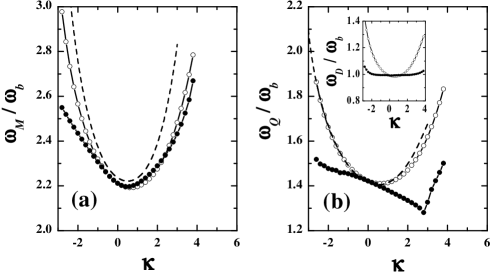
Figure 1: The dispersion relation of the monopole ($l=0$) and quadrupole ($l=2$) condensate oscillations for a mixture composed of $2\times 10^{4}$ ${}^{41}{\rm K}$ (boson) and $2\times 10^{4}$ ⁴⁰K (fermion) atoms at $T=0.01T_{c}^{0}$, where $T_{c}^{0}=0.94\omega_{b}N_{b}^{1/3}/k_{B}\approx 122$ nK is the critical temperature for an ideal Bose gas in the thermodynamic limit. The mode frequencies, in units of the bare trapping frequency, are plotted as a function of the reduced Bose-Fermi coupling, $\kappa=g_{bf}/g_{bb}$. The lines with open circles show the unperturbed frequencies calculated by the static HFB-Popov equations $\omega_{0}$, while the lines with solid circles denote $\omega=\omega_{0}+\delta\omega$. For comparison the predictions of the scaling theory in Ref. [8] are also plotted by the dashed lines. The inset in (b) shows the dispersion relation of the dipole excitation. The other parameters used in the numerical calculation are: $m_{b}=m_{f}=0.649\times 10^{-25}$ kg, $\omega_{b}=\omega_{f}=2\pi\times 100$ Hz, and $a_{bb}=286a_{0}=15.13$ nm, where $a_{0}=0.529$ ${\rm\AA}$ is the Bohr radius.

In Figs. (1a) and (1b), we present, respectively, our results for the monopole ($l=0$) and quadrupole ($l=2$) condensate oscillations at a very low temperature $T=0.01T_{c}^{0}$, where $T_{c}^{0}=0.94\omega_{b}N_{b}^{1/3}/k_{B}\approx 122$ nK is the critical temperature for an ideal Bose gas in the thermodynamic limit. The mode frequencies, in units of the bare trapping frequency, are plotted as a function of the Bose-Fermi coupling constant measured relative to the Bose-Bose coupling constant, $\kappa=g_{bf}/g_{bb}$. The lines with open circles show the unperturbed frequencies obtained from the HFB-Popov equations, $\omega_{0}$, while the lines with solid circles denote the values after correction, $\omega=\omega_{0}+\delta\omega$. For comparison, the predictions of the scaling theory at zero temperature are also plotted by the dashed lines liu . At this low temperature, the eigenfrequency shift $\delta\omega$ arises mainly from the dynamics of the degenerate Fermi gas. For small values of $\left|\kappa\right|\lesssim 1$, $\delta\omega$ is negligibly small due to square dependence on the Bose-Fermi coupling constant. However, as $\left|\kappa\right|$ increases $\delta\omega$ becomes remarkable. In particular, the corrected frequency for the quadrupole mode decreases with increasing Bose-Fermi coupling constant up to $\kappa\approx 3$, at which a sharp upturn occurs. This sharp dip is accompanied by a dramatic increase of damping rates (not shown in the figure), and can be well interpreted as a signal to approach the spatial separation (demixing) point of the two species. On the contrary, the unperturbed quadrupole frequency $\omega_{0}$ has a qualitatively different behavior against $\kappa$: it shows a parabolic dependence with a minimum located around $\kappa=0.5$. In spite of its large value at $\left|\kappa\right|\gtrsim 1$, $\delta\omega$ is still much smaller than unperturbed frequency $\omega_{0}$ for all the calculated points. Therefore, the criterium for the applicability of the perturbation theory in Eqs. (15) and (16) is justified. In the inset of Fig. (1b) we also show the result for the dipole mode ($l=1$). As we can see, although $\omega_{0}$ deviates significantly from the bare trapping frequency $\omega_{b}$ for relatively small values of $\kappa$, $\omega$ still persists at $\omega_{b}$ over a wide range of $\kappa$ (i.e., $-2\lesssim\kappa\lesssim+3$). This is consistent with the generalized Kohn theorem. As a result, the correctness of our theory and numerical calculations is partly checked.

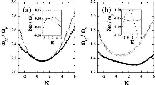
Figure 2: The same as in FIG. 1, but for $T=0.75T_{c}^{0}$. In the insets the solid and dashed lines show, respectively, the fractional shift $\delta\omega/\omega_{0}$ due to the first and second terms in Eq. (30).

The eigenfrequency shifts are affected by the temperature. In Fig. 2, we report the mode frequencies against $\kappa$ at a high temperature $T=0.75T_{c}^{0}$, where the condensate oscillates in the presence of a large fraction of above-condensate atoms. Compared with the results for the low temperature, the eigenfrequency shifts are considerably reduced. The sharp dip at $\kappa\approx 3$ for the quadrupole mode also becomes much broader. Moreover, in the absence of the Bose-Fermi coupling, the eigenfrequency shift is nonzero for the quadrupole mode. This is caused by the dynamics of the noncondensate component as shown in the inset of Fig. (2b), where the solid and dashed lines depict, respectively, the fractional shift $\delta\omega/\omega_{0}$ due to the Bose-Bose interaction and Bose-Fermi coupling (or, in other words, due to the first and second terms in Eq. (30)).

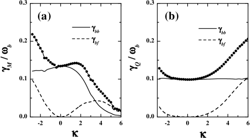
Figure 3: The damping rates of the monopole (a) and quadrupole condensate oscillations (b) at $T=0.75T_{c}^{0}$. The solid and dashed lines correspond to the contribution from the Landau process due to the Bose-Bose interaction and due to the Bose-Fermi coupling, respectively. The line with solid circles is the total contribution.

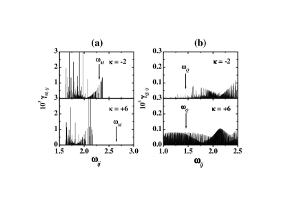
Figure 4: The damping strength $\gamma_{ij\text{ }}$defined in Eq. (32) as a function of the transition frequencies $\omega_{ij}$ (in units of $\omega_{b}$) allowed by the selection rules. (a) $\gamma_{ij\text{ }}^{bb}$ for the monopole excitation and (b) $\gamma_{ij\text{ }}^{bf}$ for the quadrupole excitation. In each subplot, upper and lower panels correspond to the case of $\kappa=-2$ and $\kappa=+6$, respectively. In the former case the mixture is in mixed regime, while in the latter the bosonic and fermionic density profiles separate in space. The arrows point to $\omega=\omega_{0}+\delta\omega$.

The damping rate of condensate oscillations at finite temperature deserves its own study. In Figs. (3a) and (3b), we show, respectively, our predictions on the damping rates of monopole and quadrupole oscillations at $T=0.75T_{c}^{0}$. The lines with solid circles are the sum over two contributions: one is the Landau damping due to the Bose-Bose interaction (the solid lines), $\gamma_{bb}$, and the other is the Landau damping due to the Bose-Fermi coupling (the dashed line), $\gamma_{bf}$. For the monopole mode, the essential feature is the decrease of the damping rate as $\kappa$ increases towards the demixing point. This decrease is mainly attributed by $\gamma_{bb}$, and reflects the reconstruction of the bosonic monopole-excitation spectrum across the demixing point. To better illustrate this point, we rewrite the expression for $\gamma$ in the following form

$$\gamma = \gamma_{bb}+\gamma_{bf},$$ (31)

$$\gamma_{bb} = 4g_{bb}^{2}\omega_{0}\sum\limits_{ij}\gamma_{ij}^{bb}\frac{\gamma/\pi}{\left[\omega_{0}+\delta\omega+\left(\omega_{i}^{B}-\omega_{j}^{B}\right)\right]^{2}+\gamma^{2}},$$

$$\gamma_{bf} = g_{bf}^{2}\omega_{0}\sum\limits_{ij}\gamma_{ij}^{bf}\frac{\gamma/\pi}{\left[\omega_{0}+\delta\omega+\left(\omega_{i}^{F}-\omega_{j}^{F}\right)\right]^{2}+\gamma^{2}},$$

where the “damping strength”

$$\gamma_{ij}^{bb} = \frac{\pi}{\omega_{0}}\left|A_{ij}\right|^{2}\left(f_{i}^{B}-f_{j}^{B}\right),$$

$$\gamma_{ij}^{bf} = \frac{\pi}{\omega_{0}}\left|C_{ij}\right|^{2}\left(f_{i}^{F}-f_{j}^{F}\right),$$ (32)

have the dimensions of a frequency. In Fig. (4a), we plot $\gamma_{ij}^{bb}$ against the transition frequency $\omega_{ij}=\omega_{j}^{B}-\omega_{i}^{B}>0$ allowed by the selection rules for $\kappa=-2$ and $\kappa=6$. For the latter value of $\kappa$, the overlap between the bosonic and fermionic cloud is very small, and the mixture is deep into the demixing regime. Compared with the mixing case of $\kappa=-2$, the region of transition frequencies at $\kappa=6$ narrows, and its center moves to the low-energy side. Contrarily the calculated $\omega_{0}+\delta\omega$ has a blue shift and is completely out of the transition region. As a consequence, the condensate oscillation is not damped by the Landau process due to the Bose-Bose interaction. For the quadrupole mode, instead we observe that the damping rate increases as the mixture moves towards the demixing point with increasing $\kappa$. This trend comes from the increase of $\gamma_{bf}$, and reflects, on the other hand, the reconstruction of the fermionic quadrupole-excitation spectrum. As shown in Fig. (4b), with increasing Bose-Fermi coupling the damping strength $\gamma_{ij}^{bf}$ becomes larger and denser. Accordingly, the condensate oscillation is heavily damped by generating many particle-hole excitations.

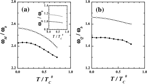
Figure 5: The dispersion relation of the monopole (a) and quadrupole excitations (b) against the reduce temperature $T/T_{c}^{0}$ at $\kappa=-2$. The inset in (a) shows the dispersion relation for the dipole mode.

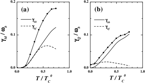
Figure 6: The same as in FIG. 5, but for the damping rates.

The last study in this subsection concerns the temperature dependence of the eigenfrequency shifts and damping rates at a specific Bose-Fermi coupling constant. In Figs. (5a) and (5b), we report, respectively, our results for the monopole and quadrupole mode frequencies as a function of the reduced temperature $T/T_{c}^{0}$ at $\kappa=-2$. The corresponding damping rates are shown in Figs. (6a) and (6b). The fulfillment of the generalized Kohn theorem is checked in the inset of Fig. (5a), where the calculated dipole frequency is very close to $\omega_{b}$ (or, more precisely, $0.97\leq\omega_{D}/\omega_{b}\leq 1.0$) for all the temperatures considered. At this specific value of $\kappa$, one can see that both the monopole and quadrupole frequencies have a downshift with increasing temperature, analogous to the results obtained for a pure Bose gas giorgini ; reidl . In addition, the behavior of the damping rates is also qualitatively similar reidl ; das ; gp .

III.2 ${}^{87}{\rm Rb}-^{40}$K

We now turn to consider a ${}^{87}{\rm Rb}-^{40}$K mixture composed of $2\times 10^{4}$ bosonic and $2\times 10^{4}$ fermionic atoms under the conditions appropriate to the LENS experiments lens . As in experiment, we introduce the quantities $\alpha=m_{f}/m_{b}=0.463$ and $\beta=$ $\omega_{f}/\omega_{b}=1.47$ to parameterize the different mass and different trapping frequency of the two species, which satisfy the constraint $\alpha\beta^{2}=1$ since both bosons and fermions experience the same trapping potential. In addition, we take the $s$-wave Bose-Bose scattering length $a_{bb}=99a_{0}=5.24$ nm heinzen , and fix the trapping frequency $\omega_{b}=2\pi\times 91.7$ Hz, which is the geometric average of the axial and radial frequencies of Ref. lens . The $s$-wave Bose-Fermi scattering length is varying, and in the experiment it can be conveniently tuned by the Feshbach resonance simoni . Notice that the calculations presented here are restricted to the isotropic traps, opposite to the cylindrical symmetric traps used in experiments. As a result, our results are only useful in a qualitatively level.

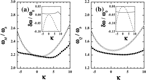
Figure 7: The dispersion relation of the monopole and quadrupole condensate excitations for a mixture consisting of $2\times 10^{4}$ ${}^{87}{\rm Rb}$ and $2\times 10^{4}$ ⁴⁰K atoms at $T=0.75T_{c}^{0}$, where $T_{c}^{0}\approx 112$ nK. The other parameters used in the calculation are: $m_{b}=1.45\times 10^{-25}$ kg, $\omega_{b}=2\pi\times 91.7$ Hz, $m_{f}/m_{b}=0.463$, $\omega_{f}/\omega_{b}=1.47$, and $a_{bb}=99a_{0}=5.24$ nm.

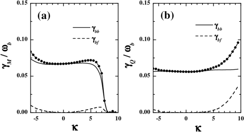
Figure 8: The same as in FIG. 7, but for the damping rates.

In Fig. 7, we plot the frequencies for the monopole and quadrupole oscillations as a function of $\kappa$ at $T=0.75T_{c}^{0}$, where $T_{c}^{0}\approx 112$ nK. Both the monopole and quadrupole frequencies decrease slowly with increasing $\kappa$ up to $\kappa\approx 5$. Above this value the frequencies gradually rise up. In the whole region of $\kappa$, the variation of frequencies due to Bose-Fermi coupling is small. However, it is still possible to be detected by the accurate frequency measurement. For instance, at $\kappa=-6$, we find that the values of the relative variation $\left(\omega_{\kappa=-6}-\omega_{\kappa=0}\right)/\omega_{\kappa=0}$ for the monopole and quadrupole modes are, respectively, $2.8\%$ and $7.6\%$, well within the experimental resolution.

The damping rate of the monopole and quadrupole modes at the same temperature is shown in Figs (8a) and (8b), respectively. The behavior of the damping rate against $\kappa$, that is, the decrease (increase) of the monopole (quadrupole) damping rate across the demixing point $\kappa\approx 5$, is very similar to that in Figs. (3a) and (3b), except that the overall magnitude is two times smaller. This behavior together with the slow rise up of the mode frequency around $\kappa\approx 5$ thus may provide us a useful signal to locate the onset of the phase transition of spatial separation.

IV concluding remarks

In this paper we have developed a theory for studying the low-lying condensate oscillations of a spherically trapped Bose-Fermi mixture at finite temperature in the collisionless regime. In this theory, the unperturbed mode frequency is firstly calculated within the static Hartree-Fock-Bogoliubov-Popov approximation. The frequency correction, arising from the coupled dynamics of the condensate, noncondensate, and degenerate Fermi gas, is then taken into account perturbatively by means of the random phase approximation. We have applied our theory to the mixtures of ${}^{41}{\rm K}-^{40}$K and ${}^{87}{\rm Rb}-^{40}$K, and have studied the dispersion relation of the monopole and quadrupole condensate excitations as a function of the Bose-Fermi coupling at various temperatures. The correctness of our theory and numerical calculations is partly checked by the fulfillment of the generalized Kohn theorem for the dipole excitation. At a relatively high temperature we find that, as the mixture moves towards demixing point with increasing Bose-Fermi coupling, the damping rate of the monopole (quadrupole) excitation increases (decreases). This behavior provides us a possible signature to identify the phase transition of spatial separation.

References

• (1) M. H. Anderson, J. R. Ensher, M. R. Matthews, C. E. Wieman, and E. A. Cornell, Science 269, 198 (1995).
• (2) K. B. Davis, M.-O. Mewes, M. R. Andrews, N. J. van Druten, D. S. Durfee, D. M. Kurn, and W. Ketterle, Phys. Rev. Lett. 75, 3969 (1995).
• (3) C. C. Bradley, C. A. Sackett, J. J. Tollett, R. G. Hulet, Phys. Rev. Lett. 75, 1687 (1995).
• (4) A. G. Truscott, K. E. Strecker, W. I. McAlexander, G. B. Partridge, and R. G. Hulet, Science 291, 2570 (2001); F. Schreck, L. Khaykovich, K. L. Corwin, G. Ferrari, T. Bourdel, J. Cubizolles, and C. Salomon, Phys. Rev. Lett. 87, 080403 (2001).
• (5) Z. Hadzibabic, C. A. Stan, K. Dieckmann, S. Gupta, M. W. Zwierlein, A. Gorlitz, and W. Ketterle, Phys. Rev. Lett. 88, 160401 (2002).
• (6) G. Roati, F. Riboli, G. Modugno, and M. Inguscio, Phys. Rev. Lett. 89, 150403 (2002); G. Modugno, G. Roati, F. Riboli, F. Ferlaino, R. J. Brecha, and M. Inguscio, Science 297, 2240 (2002).
• (7) T. Miyakawa, T. Suzuki, and H. Yabu, Phys. Rev. A 62, 063613 (2000).
• (8) X.-J. Liu and H. Hu, Phys. Rev. A 67, 023613 (2003).
• (9) P. Capuzzi and E. S. Hernández, Phys. Rev. A 64, 043607 (2001).
• (10) T. Sogo, T. Miyakawa, T. Suzuki, and H. Yabu, Phys. Rev. A 66, 013618 (2002).
• (11) A. Minguzzi and M. P. Tosi, Plys. Lett. A 268, 142 (2000).
• (12) P. Capuzzi, A. Minguzzi, and M. P. Tosi, LANL Preprint cond-mat/0301522 (2003).
• (13) H. Hu and X.-J. Liu, LANL Preprint cond-mat/0302570 (2003); to be published in Phys. Rev. A.
• (14) A. Griffin, Phys. Rev. B 53, 9341 (1996); D. A. Hutchinson, E. Zaremba and A. Griffin, Phys. Rev. Lett. 78, 1842 (1997).
• (15) R. J. Dodd, M. Edwards, C. W. Clark, and K. Burnett, Phys. Rev. A 57, R32 (1998).
• (16) S. Giorgini, Phys. Rev. A 61, 063615 (2000); ibid. 57, 2949 (1998).
• (17) M. J. Bijlsma and H. T. C. Stoof, Phys. Rev. A 60, 3973 (1999); U. Al Khawaja and H. T. C. Stoof, ibid. 62, 053602 (2000).
• (18) E. Zaremba, A. Griffin, and T. Nikuni, Phys. Rev. A 57, 4695 (1998); E. Zaremba, T. Nikuni, and A. Griffin, J. Low Temp. Phys. 116, 277 (1999); T. Nikuni, E. Zaremba, and A. Griffin, Phys. Rev. Lett. 83, 10 (1999).
• (19) P. O. Fedichev, G. V. Shlyapnikov, and J. T. M. Walraven, Phys. Rev. Lett. 80, 2269 (1998); P. O. Fedichev and G. V. Shlyapnikov, Phys. Rev. A 58, 3146 (1998).
• (20) J. Reidl, A. Csordás, R. Graham, and P. Szépfalusy, Phys. Rev. A 61, 043606 (2000).
• (21) J. E. Williams and A. Griffin, Phys. Rev. A 63, 023612 (2001); ibid. 64, 013606 (2001).
• (22) The terms cubic in the field operators in the equation of motion (2) take the form: $\psi^{+}\psi\psi=\left|\Phi\right|^{2}\Phi+2\left|\Phi\right|^{2}\tilde{\psi}+\Phi^{2}\tilde{\psi}^{+}+2\Phi\tilde{\psi}^{+}\tilde{\psi}+\Phi^{*}\tilde{\psi}\tilde{\psi}+\tilde{\psi}^{+}\tilde{\psi}\tilde{\psi}$, and $\psi\phi^{+}\phi=\Phi\phi^{+}\phi+\tilde{\psi}\phi^{+}\phi$. From the semiclassical point of view, the cubic product of the operator, $\tilde{\psi}^{+}\tilde{\psi}\tilde{\psi}$ (or $\tilde{\psi}\phi^{+}\phi$), accounts for the collisions involving the condensate and noncondensate atoms (or fermions) zgn . In the collisionless regime we may assume that these products have only a negligible effect on the dynamics of the condensate and we may safely set the triplet average value to zero: $\left\langle\tilde{\psi}^{+}({\bf r},t)\tilde{\psi}({\bf r},t)\tilde{\psi}({\bf r},t)\right\rangle=0$ and $\left\langle\tilde{\psi}({\bf r},t)\phi^{+}({\bf r},t)\phi({\bf r},t)\right\rangle=0$. On the other hand, for a pure Bose gas the damping due to collisions has been discussed by Williams and Griffin in Ref. wg . For typical trap parameters, it is found to be 2 or 3 times smaller than the Landau damping arising from the dynamical mean-field effect as discussed in the present paper. The collisional frequency shift is also considered in these papers, and found to vanish in the first order perturbation treatment.
• (23) V. N. Popov, Functional Integrals and Collective Excitations (Cambridge University Press, Cambridge, 1987).
• (24) S. Giorgini, L. P. Pitaevskii, and S. Stringari, Phys. Rev. A 54, R4633 (1996); Phys. Rev. Lett. 78, 3987 (1997).
• (25) This approximation was first used by Popov in the study of a homogeneous gas to discuss the finite temperature region close to the Bose-Einstein transition popov . More recently, the Popov approximation has been used extensively in the study of properties of magnetically trapped Bose gases at finite temperature griffin ; burnett ; gps . This Popov approximation gives a gapless spectrum of elementary excitations at long wavelengths and formally reduces to the Bogoliubov approximation at zero temperature, where $\tilde{n}^{0}({\bf r})$ also becomes negligible. While at high temperatures, it approaches the finite-temperature Hartree-Fock spectrum. Therefore it is expected to give a reasonable first approximation for the excitation spectrum in Bose gases at all temperatures griffin .
• (26) A. Griffin, Excitations in a Bose-Condensed Liquid (Cambridge, New York, 1993), Chap. 5, and references therein.
• (27) As we shall see, if we take $g_{bb}$ and $g_{bf}$ as small parameters, $\delta\tilde{n}({\bf r})$, $\delta\tilde{m}({\bf r})$, and $\delta n_{f}({\bf r})$ are an order smaller than $\delta\Phi({\bf r})$.
• (28) A. L. Fetter and J. D. Walecka, Quantum Theory of Many-Particle Systems (McGraw Hill, New York, 1971).
• (29) In other words, it arises from the process of one quantum of the condensate oscillation $\omega$ being absorbed by a fermion below the Fermi level with energy $\omega_{i}^{F}$, which is turned into a fermion above the Fermi level with energy $\omega_{j}^{F}=\omega_{i}^{F}+\omega$.
• (30) G. M. Bruun, Y. Castin, R. Dum, and K. Burnett, Eur. Phys. J. D 9, 433 (1999); G. M. Bruun and B. R. Mottelson, Phys. Rev. Lett. 87, 270403 (2001).
• (31) That is, the divergence is removed by the substitutions, $\chi_{\tilde{m}\tilde{m}^{+}}\left({\bf r},{\bf r}^{\prime};\omega\right)\rightarrow\chi_{\tilde{m}\tilde{m}^{+}}\left({\bf r},{\bf r}^{\prime};\omega\right)-\delta({\bf r}-{\bf r}^{\prime})G_{0}^{irr}({\bf r})$, and $\chi_{\tilde{m}^{+}\tilde{m}}\left({\bf r},{\bf r}^{\prime};\omega\right)\rightarrow\chi_{\tilde{m}^{+}\tilde{m}}\left({\bf r},{\bf r}^{\prime};\omega\right)-\delta({\bf r}-{\bf r}^{\prime})G_{0}^{irr}({\bf r})$. Here $G_{0}^{irr}({\bf r})$ is the singular part of the ideal single-particle Green’s function $G_{0}({\bf r+x}/2,{\bf r-x}/2;\omega=0)$ that diverges as $1/x$ for $x$ $\rightarrow 0$ bruun .
• (32) D. S. Jin, M. R. Matthews, J. R. Ensher, C. E. Wiemann, and E. A. Cornell, Phys. Rev. Lett. 78, 764 (1997).
• (33) K. Das and T. Bergeman, Phys. Rev. A 64, 013613 (2001).
• (34) R. Côté, A. Dalgarno, H. Wang, and W. C. Stwalley, Phys. Rev. A 57, R4118 (1998).
• (35) M. Guilleumas and L. P. Pitaevskii, Phys. Rev. A 61, 013602 (2000).
• (36) E. G. M. van Kempen, S. J. J. M. F. Kokkelmans, D. J. Heinzen, and B. J. Verhaar, Phys. Rev. Lett. 88, 093201 (2002).
• (37) A. Simoni, F. Ferlaino, G. Roati, G. Modugno, and M. Inguscio, Phys. Rev. Lett. 90, 163202 (2003).