Charge instabilities in strongly correlated bilayer systems

Abstract

We investigate the charge-instabilities of the Hubbard-Holstein model with two coupled layers. In this system the scattering processes naturally separate into contributions which are either symmetric or antisymmetric combinations with respect to exchange of the layers. It turns out that the short-range strong correlations suppress finite wave-vector nesting instabilities for both symmetries but favor the occurrence of phase separation in the symmetric channel. Inclusion of a sizeable long-range Coulomb (LRC) interaction frustrates the $q=0$ instabilities and supports the formation of incommensurate charge-density waves (CDW). Upon reducing doping from half-filling and for small electron-phonon coupling $g$ the CDW instability first occurs in the antisymmetric channel but both instability lines merge with increasing g. While LRC forces always suppress the phase separation instability in the symmetric channel, the CDW period in the antisymmetric sector tends to infinity ($q_{c}\to 0$) for sufficiently small Coulomb interaction. This feature allows for the possibility of singular scattering over the whole Fermi surface. We discuss possible implications of our results for the bilayer high-T_c cuprates.

I Introduction

Among the variety of cuprate superconductors most angle-resolved photoemission spectroscopy (ARPES) experiments have been made on the bilayer compound Bi₂Sr₂CaCu₂O_8+δ (Bi2212) due to the advantage of good cleavage planes and its nearly perfectly two-dimensional electronic structure. CAMP0 However, only recent improvements in the resolution of ARPES measurements allowed for the detection of the band splitting due to coherent c-axis coupling of the two layers within a unit cell . FENG ; CHUANG The same feature has also been observed in modulation-free (Bi,Pb)-2212 KORDYUK and there is experimental evidence that the magnitude of the bilayer splitting is constant over a large range of doping. CHUANG2 The splitting obeys the expected symmetry of LDA computations ANDERSEN ; LIECHTENSTEIN being essentially zero along the diagonals $(0,0)\to(\pi,\pi)$ and (in the normal state) acquires a value between 88meV FENG and 110meV CHUANG at the $(\pi,0)$ point of the Brillouin zone (BZ).

Below T_c, the ARPES spectra display additional features which can be interpreted in terms of a coupling of the charge carriers to a collective mode. As a consequence the dispersion along the nodal direction shows a break at some characteristic energy $\omega_{0}$ LANZARA with an increased effective mass for binding energies smaller than $\omega_{0}$. It has been shown that an analogous anomaly is also present in the bonding band dispersion of Bi2212 around $(\pi,0)$ (M-point) which reveals as an additional peak-dip hump feature in the ARPES line shape. GROMKO However, more recent ARPES experiments on underdoped (Bi,Pb)-2212 KIM have revealed a similar mass renormalization in bonding and antibonding band.

Concerning the physical origin of these mode-type features the various proposals include a magnetic resonance (see e.g. Refs. CAMP, ; ESCHRIG1, ; ESCHRIG2, ), the coupling to phonons LANZARA or incommensurate charge-density waves (ICDW) GOETZ ; VARL as the source of the associated scattering. Further on from neutron scattering experiments (see e.g. Ref. TRAN, ) it is known that the spin fluctuations between the layers in YBa₂CU₃O_7-δ are antiferromagnetically correlated so that the corresponding exchange potential is antisymmetric. However, since the weight of the resonance is quite small, large coupling constants are required in order to reproduce the spectral features within a magnetic mechanism and therefore this scenario is still controversially discussed. KIV

In this paper we show that antisymmetric scattering in a bilayer system is not unique to a magnetic interaction but may also occur in the charge sector close to a ICDW instability. Our analysis can be viewed as an extension of the theory proposed by Castellani et al. in Ref. CAST, according to which the anomalous electronic properties of high-T_c materials are determined by a quantum critical point (QCP) located near optimal doping. The occurence of such an instability towards ICDW formation can be theoretically substantiated by considering the interplay between phase separation (PS) and the long-range Coulomb interaction. PS is a natural feature of systems where strong electronic correlations lead to a substantial reduction of the kinetic energy. As a consequence short-range range attractive interactions (e.g. of phononic or magnetic origin) may dominate and induce a charge aggregation in highly doped metallic regions and a simultaneous charge depletion in spatially separated regions. It was pointed out in Ref. EMERY, that long-range Coulomb forces oppose the charge separation suppressing long-wavelength density fluctuations. It has been shown CAST ; BECCA that this ’frustration’ of PS may result in a finite-momentum instability corresponding to a ICDW quantum critical point. Near this instability the associated singular scattering favors the occurrence of d-wave superconductivity PERALI and can explain the anomalous hump-type absorption in the optical conductivity of overdoped cuprates. CAPRARA In addition, the strong fluctuations associated with the proximity to a QCP may account for the dependence of the pseudogap temperature on the characteristic time scale of the particular experiment. ANDERGASSEN

Further experimental evidence for the existence of a QCP in the phase diagram of high-T_c cuprates has been growing over the last few years (see e.g. Ref. EVIDENCE, and references therein). The idea that the associated order in the underdoped regime is compatible with ICDW formation is also supported by recent scanning tunneling microscopy (STM) experiments. HOWALD These measurements have revealed the existence of a non-dispersing peak in the Fourier transformed local density of states in slightly overdoped Bi2212 and thus the presence of static charge order in this compound (for a more detailed discussion on the detection of charge order in cuprates see Ref. KIV2, ).

Previous investigations of the ICDW-QCP scenario CAST ; BECCA have been based on the two-dimensional electronic structure of a single CuO₂ plane. However, real cuprate compounds can be prepared with a variable number of CuO₂ layers per unit cell which additionally are electronically coupled along the c-axis. Such a layered structure has profound consequences on the momentum dependence of the long-range Coulomb interaction and on the spectrum of low-energy collective modes. In this paper we study the simplest extension of the single-layer case, namely we investigate possible charge instabilities in a system consisting of two coupled layers. In Sec. II we introduce the Hubbard-Holstein bilayer model and outline the evaluation of the relevant effective interactions between quasiparticles within an $1/N$ expansion. In a bilayer system these interactions can be either symmetric or antisymmetric with respect to exchange of the layers. We show in Sec. IIIa that in the absence of long-range interactions and similar to the single-layer system the strong local repulsion favors the occurence of a phase separation instability in the symmetric sector. Long-range Coulomb forces are introduced in Sec. IIIb. It turns out that in this case the preferred charge-instability occurs in the antisymmetric channel although the symmetric instability line can be rather close. We finally discuss possible implications of our results for the high-T_c cuprates in Sec. IV. Since this paper extends previous calculations for single-layer systems the reader is recommended to study Ref. BECCA, for more details on the subject.

II Formalism

II.1 The Model

Starting point Hamiltonian is the Hubbard-Holstein model for two coupled layers:

$$H = \sum_{ij,\sigma,\alpha}t_{ij}f^{\dagger}_{i\sigma,\alpha}f_{j\sigma,\alpha}+\sum_{ij,\sigma}t^{\perp}_{ij}\left(f^{\dagger}_{i\sigma,1}f_{j\sigma,2}+h.c.\right)$$ (1)

$$+ U\sum_{i}n_{i\uparrow}n_{i\downarrow}-\mu_{0}\sum_{i,\alpha}n_{i\sigma,\alpha}+\omega_{0}\sum_{i,\alpha}A^{\dagger}_{i,\alpha}A_{i,\alpha}$$

$$- g\sum_{i\sigma,\alpha}\left(A^{\dagger}_{i,\alpha}+A_{i,\alpha}\right)\left(n_{i\sigma,\alpha}-\langle n_{i\sigma,\alpha}\rangle\right)$$

where $f^{(\dagger)}_{i\sigma,\alpha}$ annihilates (creates) an electron at site $R_{i}$ of layer $\alpha=1,2$ and $n_{i\sigma,\alpha}=f^{\dagger}_{i\sigma,\alpha}f_{i\sigma,\alpha}$. Note that Eq. (1) does not contain long-range forces which will be included in Sec. IIIb.

The chemical potential is denoted by $\mu_{0}$ and $t_{ij}$ and $t^{\perp}_{ij}$ are hopping amplitudes in- and between the layers, respectively. In the following we take as the Fourier transformed of the interlayer hopping

$$t^{\perp}(k)=t^{\perp}_{0}\left[\left(\cos(k_{x})-\cos(k_{y}\right))^{2}/4\right]$$ (2)

motivated by LDA calculations FENG ; CHUANG and ARPES experiments LIECHTENSTEIN for high-T_c bilayer compounds.

The operators $A_{i}^{(\dagger)}$ describe dispersionless phonons (frequency $\omega_{0}$) interacting with the electrons via a local (Holstein-type) coupling. Note that the electron-phonon coupling vanishes on the mean-field level since it is incorporated only via the density fluctations COMM .

Furtheron we take the limit $U\to\infty$ which can be considered within a standard slave-boson technique. SLABOS ; RADGAUGE In order to implement the constraint of no double occupation the original fermion operators are decomposed as $f^{\dagger}_{i\sigma,\alpha}\rightarrow c^{\dagger}_{i\sigma,\alpha}b_{i\alpha},\,\,\,{f}_{i\sigma,\alpha}\rightarrow b^{\dagger}_{i\alpha}c_{i\sigma,\alpha}$. Moreover it is convenient to introduce the limit of large orbital degeneracy N to introduce a small parameter $1/N$ for a perturbative expansion. The new fermion and boson operators are related by the constraint

$$\sum_{\sigma}c_{i\sigma\alpha}^{\dagger}c_{i\sigma\alpha}+b_{i\alpha}^{\dagger}b_{i\alpha}=N/2$$ (3)

which is implemented below by introducing an additional local Lagrange multiplier $\lambda_{i\alpha}$. Within the large N expansion the model can then be represented as a functional integral

$$Z = \int Dc^{\dagger}_{\sigma}Dc_{\sigma}Db^{\dagger}DbD\lambda DADA^{\dagger}e^{-\int_{0}^{\beta}Sd\tau},$$ (4)

$$S = \sum_{i}\left[\sum_{\sigma}c^{\dagger}_{i\sigma}{{\partial c_{i\sigma}}\over{\partial\tau}}+b^{\dagger}_{i}{{\partial b_{i}}\over{\partial\tau}}+A^{\dagger}_{i}{{\partial A_{i}}\over{\partial\tau}}\right]+H$$ (5)

with

$$H = \frac{1}{N}\sum_{ij,\sigma,\alpha}t_{ij}c^{\dagger}_{i\sigma,\alpha}c_{j\sigma,\alpha}b^{\dagger}_{j,\alpha}b_{i,\alpha}+\sum_{i\sigma,\alpha}(-\mu_{0}+i\lambda_{i,\alpha})n_{i\sigma,\alpha}$$ (6)

$$+ \frac{1}{N}\sum_{ij,\sigma}t^{\perp}_{ij}\left(c^{\dagger}_{i\sigma,1}c_{j\sigma,2}b^{\dagger}_{j,2}b_{i,1}+H.c.\right)+\omega_{0}\sum_{i,\alpha}A^{\dagger}_{i,\alpha}A_{i,\alpha}$$

$$+ \sum_{i,\alpha}i\lambda_{i,\alpha}\left(b^{\dagger}_{i,\alpha}b_{i,\alpha}-{N\over 2}\right)$$

$$- \frac{g}{\sqrt{N}}\sum_{i\sigma,\alpha}\left(A^{\dagger}_{i,\alpha}+A_{i,\alpha}\right)\left(n_{i\sigma,\alpha}-\langle n_{i\sigma,\alpha}\rangle\right)$$

where we have rescaled the hopping $t^{(\perp)}_{ij}\to t^{(\perp)}_{ij}/N$ and the el.-ph. coupling constant $g\to g/\sqrt{N}$ in order to compensate for the presence of N fermionic degrees of freedom per site. The average number of particle per cell and plane is $n=n_{1}=n_{2}=(1-\delta)N/2$ and $\delta=0$ corresponds to half-filling, when one half electron per cell and per spin flavor is present in the system.

The mean-field self-consistency equations are obtained by requiring the stationarity of the mean-field free energy and they determine the values of $\langle b_{i,1}\rangle^{2}=\langle b_{i,2}\rangle^{2}=b_{0}^{2}\equiv Nr_{0}^{2}$ and of $\lambda_{0}\equiv\langle\lambda_{i,1}\rangle=\langle\lambda_{i,1}\rangle$. Then the mean-field Hamiltonian reads

$$H_{MF} = \sum_{k\sigma}\left[(E_{k}^{A}-\mu)f^{A\dagger}_{k\sigma}f^{A}_{k\sigma}+(E_{k}^{B}-\mu)f^{B\dagger}_{k\sigma}f^{B}_{k\sigma}\right]$$ (7)

$$+ 2N_{L}N\lambda_{0}\left(r_{0}^{2}-{1\over 2}\right)$$

where we have transformed to the bonding/antibonding representation for the fermionic operators

$$f^{A}_{k\sigma} = \frac{1}{\sqrt{2}}\left(c_{k\sigma,1}+c_{k\sigma,2}\right)$$ (8)

$$f^{B}_{k\sigma} = \frac{1}{\sqrt{2}}\left(c_{k\sigma,1}-c_{k\sigma,2}\right)$$ (9)

and the respective energies are given by $E_{k}^{A/B}=r_{0}^{2}(\varepsilon_{k}\pm t^{\perp}(k))$. $\varepsilon_{k}$ is the bare in-plane dispersion which comprises nearest (t) and next-nearest neighbor ($t^{\prime}=\gamma t$) hopping

$$\varepsilon_{k}=-2t[\cos(k_{x})+\cos(k_{y})+2\gamma\cos(k_{x})\cos(k_{y})]$$ (10)

and $N_{L}$ denotes the number of sites per plane. Note that at this level the square of the mean-field value of the slave-boson field $b_{0}$, $b_{0}^{2}=Nr_{0}^{2}=N\delta/2$, multiplicatively reduces both the inter- and intralayer hopping. Fig. 1 shows the bonding and antibonding band for selected cuts through the Brillouin zone. According to our choice for the interlayer hopping Eq. (2) the splitting is largest at the $(\pi,0)$ points and reduces to $t^{\perp}_{0}$ along the zone diagonals.

Figure 1: Bonding and antibonding bands with respect to the Fermi level for parameters $\gamma=-0.2$, $t^{\perp}_{0}=0.2$, and doping $\delta=0.15$. Energies are measured in units of t.

As far as $\lambda_{0}$ is concerned, this quantity rigidly shifts the bare chemical potential $\mu_{0}$ as a function of doping and is self-consistently determined by the following equation

$$\lambda_{0}= - \frac{1}{2N_{L}}\sum_{k}\left(\varepsilon_{k}+t^{\perp}(k)\right)f(E^{A}_{k})$$ (11)

$$- \frac{1}{2N_{L}}\sum_{k}\left(\varepsilon_{k}-t^{\perp}(k)\right)f(E^{B}_{k})$$

where $f(E)$ is the Fermi function.

The presence of the coupling with the phonons introduces new physical effects when one considers the fluctuations of the bosonic fields. Since only a particular combination $a=(A^{{\dagger}}+A)/(2\sqrt{N})$ of the phonon fields $A$ and $A^{{\dagger}}$ is coupled to the fermions, it is more natural to use the field $a$ and to integrate out the orthogonal combination ${\widetilde{a}}=(A-A^{{\dagger}})/(2\sqrt{N})$. Then the quadratic action for the boson field $a$ reads

$$H_{\rm{phon}}=N\sum_{n,i,\alpha}{{\omega_{n}^{2}+\omega_{0}^{2}}\over{\omega_{0}}}a_{i,\alpha}^{\dagger}a_{i,\alpha}\,\,,$$ (12)

where we have transformed the imaginary time into Matsubara frequencies. Moreover, it is convenient to work in the radial gauge RADGAUGE , the phase of the field $b_{i,\alpha}=\sqrt{N}r_{i,\alpha}\exp(-i\phi)$ is gauged away and only the modulus field $r_{i,\alpha}$ is kept, while $\lambda_{i,\alpha}$ acquires a time dependence $\lambda_{i,\alpha}\to\lambda_{i,\alpha}+\partial_{\tau}\phi_{i,\alpha}$. Thus one can define two three-component fields ${\cal A}_{\alpha}^{\mu}=(\delta r_{\alpha},\,\,\,\delta\lambda_{\alpha},\,\,\,a_{\alpha})$ where the time- and space-dependent components are the fluctuating part of the boson fields $r_{i,\alpha}=r_{0}\left(1+\delta r_{i,\alpha}\right)$, $\lambda_{i,\alpha}=-i\lambda_{0}+\delta\lambda_{i,\alpha}$ and $a_{i,\alpha}$.

Writing the Hamiltonian of coupled fermions and bosons as $H=H_{MF}+H_{\rm{bos}}+H_{\rm{int}}$, where $H_{MF}$ is the above mean-field Hamiltonian, which is quadratic in the fermionic fields, $H_{\rm{bos}}$ is the purely bosonic part, also including the terms with the $a$, $r$ and $\lambda$ bosons appearing in the action (5) and in $H_{\rm{phon}}$, Eq.(12). $H_{\rm{int}}$ contains the fermion-boson interaction terms. The inter- and intralayer hopping terms in the bilayer $U=\infty$ Hubbard model give rise to a leading order self-energy contribution in the quadratic part of the bosonic Hamiltonian

$$\Sigma^{intra}(q) = \frac{r_{0}^{2}}{2N_{L}}\sum_{k}\varepsilon_{k-q}\left[f(E^{A}_{k})+f(E^{B}_{k})\right]$$ (13)

$$\Sigma^{inter}(q) = \frac{r_{0}^{2}}{2N_{L}}\sum_{k}t^{\perp}(k-q)\left[f(E^{A}_{k})-f(E^{B}_{k})\right].$$

For the following it is more convenient to transform also the bosonic fields to symmetric and antisymmetric combinations respectively, i.e. $\widetilde{\cal A}^{\mu}_{\pm}=\frac{1}{\sqrt{2}}\left({\cal A}_{1}^{\mu}\pm{\cal A}_{2}^{\mu}\right)$ which we combine into a single vector as $\widetilde{\cal A}=(\widetilde{\cal A}_{+},\widetilde{\cal A}_{-})$.

After Fourier transformation to momentum space, the bosonic part of the action reads

$$H_{\rm{bos}}=N\sum_{q\mu\nu}\widetilde{\cal A}^{\mu}(q)B^{\mu\nu}(q)\widetilde{\cal A}^{\nu}(-q)$$

without explicitly indicating the frequency dependence for the sake of simplicity and $\mu,\nu=r_{+},\lambda_{+},a_{+},r_{-},\lambda_{-},a_{-}$. The matrix $B^{\mu,\nu}$, can be explicitely determined from Eqs.(5)-(13) which results in the following block diagonal structure

$$\underline{\underline{\bf B}}=\left(\begin{array}[]{cc}\underline{\underline{\bf B^{+}}}&{\bf 0}\\ {\bf 0}&\underline{\underline{\bf B^{-}}}\end{array}\right)$$ (14)

and $\underline{\underline{\bf B^{\pm}}}$ denote the $3\times 3$ matrices

$$\underline{\underline{\bf B^{\pm}}}=\left(\begin{array}[]{ccc}r_{0}^{2}\lambda_{0}+\Sigma^{intra}\pm\Sigma^{inter}&ir_{0}^{2}&0\\ ir_{0}^{2}&0&0\\ 0&0&\frac{\omega_{n}^{2}+\omega_{0}^{2}}{\omega_{0}}\end{array}\right).$$ (15)

The last ingredients of our perturbation theory are the vertices coupling the quasiparticles to the bosons. Similar to the bosonic fields we combine them into two three-component vectors $\widetilde{\bf\Lambda_{nm}}=\left(\widetilde{\bf\Lambda_{+,nm}},\widetilde{\bf\Lambda_{-,nm}}\right)$ allowing us to write the interaction part of the Hamiltonian in the form

$$H_{\rm{int}}=\frac{1}{2N_{L}}\sum_{k,q,\sigma}\sum_{nm\mu\nu}f^{n,\dagger}_{k+{q\over 2}\sigma}\widetilde{\Lambda}^{\mu}_{nm}\left(k,q\right)f^{m}_{k-{q\over 2}\sigma}\widetilde{\cal A}^{\mu}\left(q\right).$$ (16)

where the indices $(nm)$ label the bonding and antibonding band respectively. It turns out that only the following vertices give rise to a non-vanishing coupling

$$\widetilde{\bf\Lambda_{+,nn}} = \left(\begin{array}[]{c}E_{k+{q\over 2}}^{n}+E_{k-{q\over 2}}^{n}\\ i\\ -2g\end{array}\right)$$ (20)

$$\widetilde{\bf\Lambda_{-,AB}} = \left(\begin{array}[]{c}E_{k+{q\over 2}}^{A}+E_{k-{q\over 2}}^{B}\\ i\\ -2g\end{array}\right)$$ (24)

$$\widetilde{\bf\Lambda_{-,BA}} = \left(\begin{array}[]{c}E_{k-{q\over 2}}^{A}+E_{k+{q\over 2}}^{B}\\ i\\ -2g\end{array}\right)$$ (28)

We are now in the position to evaluate the self-energy corrections to the boson-propagators

$$D^{\mu\nu}(q,\omega_{m})=\langle\widetilde{\cal A}^{\mu}(q,\omega_{m})\widetilde{\cal A}^{\nu}(-q,-\omega_{m})\rangle$$ (29)

which can be obtained from Dyson’s equation

$$\underline{\underline{\bf D}}=\underline{\underline{\bf D^{0}}}-\underline{\underline{\bf D^{0}}}\underline{\underline{\bf\Pi}}\underline{\underline{\bf D}}.$$ (30)

The zero order boson propagator is

$$\underline{\underline{\bf D^{0}}}=\frac{1}{2N}\underline{\underline{\bf B^{-1}}}$$ (31)

so that

$$\underline{\underline{\bf D}}=[2N\underline{\underline{\bf B}}+\underline{\underline{\bf\Pi}}]^{-1}.$$ (32)

The factor 2 multiplying the boson matrix B arises from the fact that the bosonic fields in the radial gauge are real and $\underline{\underline{\bf\Pi}}$ are just fermionic bubbles with insertion of quasiparticle-boson vertices

$$\Pi^{\mu\nu}(q,\omega_{m}) = \frac{N}{2N_{L}}\sum_{k}\sum_{st}{{f\left(E^{s}_{k+{q\over 2}}\right)-f\left(E^{t}_{k-{q\over 2}}\right)}\over{E^{s}_{k+{q\over 2}}-E^{t}_{k-{q\over 2}}-i\omega_{m}}}$$ (33)

$$\times {\Lambda}_{st}^{\mu}\left(k,q\right){\Lambda}_{ts}^{\nu}\left(k,-q\right).$$

From the structure of the vertices Eqs. (28) one can see that also $\underline{\underline{\bf\Pi}}$ acquires a block diagonal structure

$$\underline{\underline{\bf\Pi}}=\left(\begin{array}[]{cc}\underline{\underline{\bf\Pi^{+}}}&{\bf 0}\\ {\bf 0}&\underline{\underline{\bf\Pi^{-}}}\end{array}\right)$$ (34)

with $\underline{\underline{\bf\Pi^{\pm}}}$ being symmetric $3\times 3$ matrices.

Possible charge instabilities of the system can be deduced from divergencies in the corresponding correlation functions or scattering amplitudes. ABRIK The above formal scheme allows to calculate the leading-order expressions of the scattering amplitude both in the particle-hole channel

$$\Gamma_{nm;st}(k,k^{\prime};q,\omega)=-{1\over 2}\sum_{\mu\nu}{\Lambda}_{nm}^{\mu}\left(k^{\prime},-q\right)D^{\mu\nu}\left(q,\omega\right){\Lambda}_{st}^{\nu}\left(k,q\right)$$ (35)

and in the particle-particle channel

$$\Gamma_{nm;st}^{C}(k,k^{\prime};\omega)=-{1\over 2}\sum_{\mu\nu}{\Lambda}_{nm}^{\mu}\left({k+k^{\prime}\over 2},k^{\prime}-k\right)$$ (36)

$$\times D^{\mu\nu}(k-k^{\prime},\omega){\Lambda}_{st}^{\nu}\left(-{k+k^{\prime}\over 2},k-k^{\prime}\right)$$

It should be noted that the boson propagators are of order 1/N (cf. Eq. (31)) while the occurrence of a bare fermionic bubble leads to a spin summation and is therefore associated with a factor N (cf. Eq. (33)). From Eq. (32) it thus follows that in this 1/N approach the quasiparticle scattering amplitudes are residual interactions of order 1/N.

Since both the boson matrix $\underline{\underline{\bf B}}$ and the polarizability matrix $\underline{\underline{\bf\Pi}}$ are block diagonal the same also holds for the scattering amplitudes. Moreover for the scattering of two quasiparticles on the Fermi surface ($k=k_{F};k^{\prime}=k^{\prime}_{F}$) one has only two different elements for the effective scattering amplitude and we find in the particle-hole channel

$$\Gamma_{S} \equiv \Gamma_{AA;AA}=\Gamma_{AA;BB}=\Gamma_{BB;BB}=\Gamma_{BB;AA}$$

$$\Gamma_{A} \equiv \Gamma_{AB;AB}=\Gamma_{BA;BA}=\Gamma_{AB;BA}=\Gamma_{BA;AB}$$

with

$$\Gamma_{S/A}(k_{F},k^{\prime}_{F},q,\omega)=\frac{{B^{\pm}_{11}\over\delta^{2}}-{g^{2}\over B_{33}}+{\Pi^{\pm}_{11}\over 4\delta^{2}}-{2E_{F}\over\delta}-{E_{F}^{2}\over\delta^{2}}\Pi^{\pm}_{22}+i{E_{F}\over\delta^{2}}\Pi^{\pm}_{12}}{1+\left({B^{\pm}_{11}\over\delta^{2}}-{g^{2}\over B_{33}}\right)\Pi^{\pm}_{22}-i{\Pi^{\pm}_{12}\over\delta}+{\Pi^{\pm}_{11}\Pi^{\pm}_{22}-(\Pi^{\pm}_{12})^{2}\over 4\delta^{2}}}.$$ (37)

For later use we also report here the evaluation of the density-density response function which for the bilayer system is denoted as

$$P_{st,nm}(q,i\omega)=\langle T\rho^{st}(q,i\omega)\rho^{nm}(q,-i\omega)\rangle$$ (38)

where $\rho^{st}(q)=\sum_{k,\sigma}f_{k+q,\sigma}^{n\dagger}f_{k,\sigma}^{m}$ and the indices $\{s,t,n,m\}=\{A,B\}$ refer to bonding and antibonding band states, respectively. The density-density response is most conveniently expressed via the particle-hole scattering amplitudes which yields

$$P_{st,nm}(q,i\omega)=P^{0}_{st,nm}(q,i\omega)-\frac{N}{N_{L}}\sum_{kk^{\prime}}\frac{f(E_{k+{q\over 2}}^{t})-f(E_{k-{q\over 2}}^{s})}{E_{k+{q\over 2}}^{t}-E_{k-{q\over 2}}^{s}-i\omega}\Gamma_{mn,ts}^{\pm}(k,k^{\prime},q,i\omega)\frac{f(E_{k^{\prime}+{q\over 2}}^{n})-f(E_{k^{\prime}-{q\over 2}}^{m})}{E_{k^{\prime}+{q\over 2}}^{n}-E_{k^{\prime}-{q\over 2}}^{m}-i\omega}$$ (39)

The explicit form of the zero-order bubbles $P^{0}_{st,nm}(q,i\omega)$ is reported in Eqs. (57,58) and from the block-diagonal structure of the scattering amplitude it follows that also the elements of $P_{st,nm}(q,i\omega)$ decouple into the symmetric and antisymmetric sector.

Additionally we report an approximate derivation for the scattering amplitudes in appendix A which neglects the k-dependence of the vertices. This approach provides a more direct insight in the basic physical aspects of the problem and we refer to it in the following where appropriate.

III Results

III.1 Phase Separation

Let us first consider the system without long-range forces. In this case our model is characterized by strong on-site correlations which enable the electron-lattice coupling to drive the system towards a phase separation instability due to the strong reduction of the kinetic energy of the charge carriers. In the bilayer system the occurrence of a phase separation instability is signalled by a diverging scattering amplitude $\Gamma_{S}$ in the symmetric sector (cf. Eq. (37)) in the limit $\omega=0$, $q\to 0$. Since for zero temperature and $q\to 0$ the numerator of the fermionic bubbles Eq. (33) in the symmetric sector corresponds to a delta-function ($f\left(E^{s}_{k+0}\right)-f\left(E^{s}_{k-0}\right)\sim\delta(E^{s}_{k}-\mu)$) the sum over k-states only picks up contributions at the Fermi energy and as a consequence the approximative scheme described in appendix A becomes exact. Thus the instability criterion for PS in the bilayer system follows from Eqs. (63,64) and reads as

$$1+\Gamma_{S}^{0}(0)\left[N_{A}(0)+N_{B}(0)\right]=0.$$ (40)

Here $N_{A/B}(0)$ refer to the density of states of bonding and antibonding band at the chemical potential and $\Gamma_{S}^{0}$ is defined in Eq. (A). It is interesting to observe that to lowest order there is no influence of $t^{\perp}$ onto the PS instability. Since $\Sigma^{inter}<0$ one could conclude from Eq. (A) that interlayer charge fluctuations work cooperatively with the electron-phonon interaction and support the PS instability. However, interlayer hopping simultaneously enhances the kinetic energy which reflects in an enhancement of the Lagrange parameter $\lambda_{0}$ (cf. Eq. (11)). In fact, the self-energy contributions cancel out the $\lambda_{0}$ term in the 2nd order scattering amplitude $\Gamma_{S}^{0}$ which reads as $\Gamma_{S}^{0}(\omega=0,q\to 0)=\frac{1}{N}[-2E_{F}/\delta-g^{2}/\omega_{0}]$ and only indirectly depends on the interlayer hopping via the Fermi energy. Here the term proportional to the Fermi energy ($E_{F}<0$) corresponds to the residual repulsion between the quasiparticles on the Fermi surface. Despite the fact that we started from a infinite on-site repulsion between bare particles the large screening in the system gives rise to a finite scattering amplitude $\Gamma_{S}$. Therefore the additional el.-ph. coupling can always turn the interaction into an attractive one and eventually drive the system towards phase separation.

In order to analyze in more detail the $q=0$ instabilities in the symmetric and antisymmetric sector it is instructive to modify the model in Eq. (6) by coupling the phonons to the full electron density rather than to density fluctuations. In this way an el.-ph. coupling is effective already at the mean-field level, where a nonzero mean-field value of the phonon field arises in both symmetric ($a^{0}_{+}=\langle a_{+}\rangle$) and antisymmetric ($a_{-}^{0}=\langle a_{-}\rangle$) combinations. It is then straightforward to show that $\langle a_{+}\rangle$ induces a doping dependent correction to the chemical potential and Eq. (40) is identical to the condition of a stationary point in $\mu(\delta)$, signaling a divergence in the compressibility $\kappa=-\partial\delta/\partial\mu$, i.e. phase separation (cf. appendix in Ref. BECCA, ). On the other hand the instability in the antisymmetric sector corresponds to a second order phase transition where the order parameter $\langle a_{-}\rangle$ starts to acquire a finite value. As a consequence of different distortions in the two planes also the corresponding charge densities will be different.

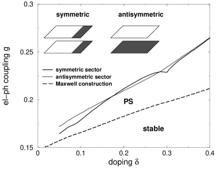
Figure 2: Phase diagram electron-phonon coupling $g$ versus doping $\delta$ for $q=0$ instabilities. The Maxwell construction for the (symmetric) phase transition separates the stable from the phase separated region. Parameters: $t=$1eV, $\gamma=-0.2$, $t^{0}_{\perp}/t=0.2$. The inset sketches the symmetry-broken state within the symmetric (i.e. PS) and antisymmetric channel. Shaded areas indicate enhanced charge density.

Fig. 2 displays the phase diagram el.-ph. coupling $g$ versus doping $\delta$ together with a sketch to elucidate the symmetric and antisymmetric $q=0$ instabilities. For the PS instability line the van-Hove singularities of bonding (BB) and antibonding band (AB) reflect as the two kinks at $\delta\approx 0.1$ and $\delta\approx 0.3$, respectively. The concentration range in between is characterized by an AB Fermi surface (FS) centered around $\Gamma=(0,0)$ and a BB FS centered around $X=(\pi,\pi)$. Since evaluation of the fermionic bubbles in the antisymmetric sector Eq. (33) requires the summation over an area which is determined by the difference of BB and AB Fermi surfaces, $\Gamma_{A}$ is strongly enhanced for $0.1<\delta<0.3$. It is therefore within this concentration range where the antisymmetric 2nd order phase transition occurs before the phase separation instability. However, a Maxwell construction has to be done in order to properly determine the coexistence region in the symmetric sector. The corresponding phase boundary is shown by the dashed line in Fig. 2. From this Maxwell construction we thus conclude that also in a bilayer system which is strongly susceptible to a 2nd order instability in the antisymmetric sector the presence of strong correlations favors the transition towards a phase separated regime.

In principle our previous analysis does not exclude the occurrence of a nesting induced phase transition before the PS instability line is reached. In order to demonstrate that the instability really takes place at wave vector $q=0$ we report in Fig. 3 the static scattering amplitudes in the particle-hole channel $\Gamma_{S/A}(k_{F},k^{\prime}_{F},q,\omega=0)$ obtained from Eq. (37) for a fixed doping $\delta=0.25$ and tuning the el.-ph. coupling towards the instabilities. In the absence of el.-ph. coupling ($g=0$) the interaction between quasiparticles is repulsive (i.e. $\Gamma>0$) in both the symmetric and antisymmetric channel. Due to the strong local correlations this residual repulsion increases with increasing wave vector $q$ in both channels. Upon switching on the el.-ph. coupling $\Gamma_{S/A}(k_{F},k^{\prime}_{F},q,\omega=0)$ therefore becomes attractive for small $q$ and diverges at some critical value $g_{crit}$. Note that results in Fig. 3 are evaluated for doping $\delta=0.25$ where the instability in the antisymmetric sector occurs first. For this reason $\Gamma_{A}$ becomes more negative for $q\rightarrow 0$ than $\Gamma_{S}$.

Figure 3: Scattering amplitudes in the symmetric (a) and antisymmetric (b) channel for a scan along $(q_{x},0)$. The three curves correspond to el.-ph. couplings $g=0.2,0.21,0.22$ respectively. Parameters: $\gamma=-0.2$, $t^{0}_{\perp}/t=0.2$, doping $\delta=0.25$.

Let us now turn to the dynamical properties in the absence of long-range interactions. Since we consider a strongly correlated bilayer system the zero sound mode consists of two branches. The acoustic one in the symmetric sector disperses as $\omega_{s}=v_{F}\sqrt{1+\tilde{u}}q$ for a 2-d system and an effective interaction $\tilde{u}$. STERN A second, optical branch exists in the antisymmetric sector and its energy scale is determined by the interlayer hopping $\omega_{a}\sim t^{\perp}$. As a consequence the Boson propagator Eq. (32) has two poles for each symmetry: one is the phonon and the other is the zero sound (which in the symmetric sector becomes the 2-d plasmon when long-range Coulomb forces are included). The two modes would cross each other (at rather small $q\sim\omega_{0}/v_{F}$) if the phonon were decoupled from the fermions but repel when the coupling is switched on. Consequently one observes two spectral features in each channel. For the symmetric combination (and small $q$): (a) the zero sound at low energy which upon increasing $g$ is pushed down and, becoming softer and softer, drives the PS; (b) the phonon mode at energy higher than $\omega_{0}$ which is hardened since it is pushed up by the repulsion with the zero sound. For the antisymmetric channel (a) at low momenta and small energies appears the phonon which now upon increasing $g$ softens towards the 2nd order instability and (b) at higher frequencies the zero sound optical mode which for larger momenta is rapidly shifted to higher frequencies and loses intensity. In Fig. 4 we show the dispersion of these excitations along the $(1,0)$ direction which can be obtained from the poles of $\Gamma_{S/A}(k_{F},k^{\prime}_{F},q,\omega)$ in Eq. (37).

Figure 4: Phonon and zero sound dispersions along the $(q_{x},0)$ direction in the symmetric ($\omega^{+}$,solid) and antisymmetric ($\omega^{-}$, dot-dashed) channel. Parameters: $\gamma=-0.2$, $t^{0}_{\perp}/t=0.2$, $g=0.22$, $\omega_{0}=0.04$,doping $\delta=0.25$.

Figure 5: Sketch of the bilayer structure which is used for evaluation of the inter- and intralayer Coulomb interaction

III.2 Inclusion of long-range interactions

The nature of possible instabilities in the system (i.e. phase separation or finite-q charge instabilities) crucially depends on the structure of the long-range Coulomb (LRC) potential in the bilayer system. Although we expect the effect of LRC forces to be most effective in the small momentum-transfer case, where the underlying lattice structure is less visible, we explicitely take into account the real symmetry of the bilayer square-lattice system (cf. Fig. 5).

The intra- and interlayer contributions to the Coulomb potential are derived in appendix B and give rise to the following interaction part of the Hamiltonian

$$H_{C}=\frac{1}{2N}\sum_{q,\mu,\nu=1,2}V_{\bf q}^{\mu\nu}\rho_{q}^{\mu}\rho_{q}^{\nu}.$$ (41)

where

$$V_{\bf q}^{\mu=\nu} = V^{intra}_{{\bf q}_{\parallel}}(z=0)$$ (42)

$$= -{V_{C}\over 2}\frac{A(q_{x},q_{y})}{\sqrt{\left[\frac{A^{2}(q_{x},q_{y})-1}{2\kappa(1-\kappa)}+1\right]^{2}-1}}$$

$$V_{\bf q}^{\mu\neq\nu} = V^{inter}_{{\bf q}_{\parallel}}(z=0)$$ (43)

$$= {V_{C}\over 2}\left\{\frac{1+{1\over 2}\frac{1}{1-\kappa}[A^{2}(q_{x},q_{y})-1]}{\sqrt{\left[\frac{A^{2}(q_{x},q_{y})-1}{2\kappa(1-\kappa)}+1\right]^{2}-1}}-\kappa\right\}.$$

The Coulombic coupling constant $V_{C}=e^{2}a_{z}/(2\epsilon_{\perp}a_{xy}^{2})$ has to range from roughly 0.5-3eV in order to have holes in neighboring CuO₂ cells repelling each other with a strength of 0.1-0.6 eV. Concerning the lattice parameters typical values in case of YBCO are $\kappa=d/a_{z}\approx 0.36$ and $a_{xy}/a_{z}\approx 0.32$. Note that $V_{\bf q}^{\mu\nu}$ is the potential between electrons in a two-dimensional bilayer lattice and the small momentum behavior reads as

$$V^{intra}_{\bf q} = \frac{V_{C}}{\sqrt{8\tilde{\epsilon}a_{z}^{2}}}{1\over q}$$ (44)

$$V^{inter}_{\bf q} = V^{intra}_{\bf q}-\kappa\frac{V_{C}}{2}.$$ (45)

Upon transforming the Coulomb potential to the (anti)symmetric representation

$$V_{S/A}(q)={1\over{2}}\left[V^{intra}_{Coul}(q)\pm V^{inter}_{Coul}(q)\right]$$ (46)

it thus turns out that the Coulombic contribution approaches a constant value ($\approx 0.1...0.5eV$ depending on parameters) in the antisymmetric sector for small momentum transfer whereas the $q=0$ divergence in the symmetric part of the interaction naturally leads to a suppression of phase separation as we will demonstrate in the next section.

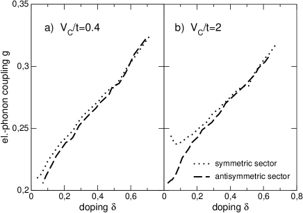
Figure 6: ICDW instability lines in the phase diagram electron-phonon coupling $g$ versus doping $\delta$. a) $V_{C}/t=0.4$; b) $V_{C}/t=2$. Parameters: $\gamma=-0.4$, $\omega_{0}/t=0.04$, $t^{0}_{\perp}/t=0.2$,$V_{C}/t=2$,$\tilde{\epsilon}=6$, $d/a_{z}=0.5$, $a_{xy}/a_{z}=0.32$.

III.3 Analysis of CDW instabilities

The analysis of possible instabilities under the presence of long-range interactions is most conveniently carried out by calculating the density-density response function $P^{LR}(q,\omega)$. Using the corresponding short-range part $P^{LR}(q,\omega)$ Eq. (39) one can perform the following resummation

$$\underline{\underline{\bf P^{LR}}}=\underline{\underline{\bf P^{SR}}}+\underline{\underline{\bf P^{SR}}}\,\,\underline{\underline{\bf V^{Coul}}}\,\,\underline{\underline{\bf P^{LR}}}$$ (47)

where the matrix $\underline{\underline{\bf V^{Coul}}}$ is given by

$$\underline{\underline{\bf V^{Coul}}}=\left(\begin{array}[]{cccc}V^{S}(q)&V^{S}(q)&0&0\\ V^{S}(q)&V^{S}(q)&0&0\\ 0&0&V^{A}(q)&V^{A}(q)\\ 0&0&V^{A}(q)&V^{A}(q)\end{array}\right).$$ (48)

Inverting Eq. (47) yields

$$\underline{\underline{\bf P^{LR}}}=[\underline{\underline{\bf 1}}-\underline{\underline{\bf P}}\,\,\underline{\underline{V^{Coul}}}]^{-1}\underline{\underline{\bf P^{SR}}}$$ (49)

so that the instabilities can be obtained from

$$DET(\underline{\underline{\bf 1}}-\underline{\underline{\bf PV^{Coul}}})=0=\left\{\begin{array}[]{l}1-V^{S}(q)[P_{AA,AA}^{SR}(q,0)+P_{AA,BB}^{SR}(q,0)+P_{BB,AA}^{SR}(q,0)+P_{BB,BB}^{SR}(q,0)]\\ 1-V^{A}(q)[P_{AB,AB}^{SR}(q,0)+P_{AB,BA}^{SR}(q,0)+P_{BA,AB}^{SR}(q,0)+P_{BA,BA}^{SR}(q,0)]\end{array}\right.$$ (50)

for the symmetric and antisymmetric channel respectively. First it should be noted that a diverging short-range density-density response no longer results in a $q=0$ instability under the presence of long-range interactions. This is particularly obvious in the symmetric channel where the Coulomb potential behaves as $V^{S}(q\to 0)\to\infty$. Thus one always finds a vanishing compressibility and phase separation is now ruled out. However, in the antisymmetric channel a diverging short-range response $P^{SR}_{n\neq m}(q\to 0,0)\to-\infty$ leads to a finite value of the corresponding long-range polarizability $P^{LR}_{n\neq m}(q=0,0)\sim-1/V^{A}(q=0)=-2a_{z}/(dV_{c})$ according to Eqs. (44-46). Thus in this case LRC interactions leave the system to some extend susceptible to long-wavelength antisymmetric density fluctuations.

Concerning possible instabilities under the presence of long-range forces the conditions in Eq. (50) can be in principle fulfilled inside the (short-range) instability regions of symmetric and antisymmetric channel where $P^{SR}_{nm}(q,0)$ has a positive branch up to some finite wave vector. Due to the fact that $P^{LR}_{n\neq m}(q=0,0)$ stays finite the antisymmetric CDW instability can even occur at arbitrarily small wave vectors depending on the strength of the LRC interaction.

Fig. 6 depicts the phase diagram el.-ph. coupling versus doping for two values of the Coulomb interaction. Up to doping $\delta\approx 0.4...0.5$ the antisymmetric instability occurs at smaller coupling $g$ than the symmetric one whereas both instability lines merge for larger concentrations. This behavior is best understood within the approximate formalism given in the appendix. The corresponding RPA equations for the effective interactions Eqs. (63,64) suggest that instabilities are favored for those wave-vectors $q_{crit}$ and dopings where (a) the residual quasiparticle interactions $\Gamma^{0}_{S}$ and $\Gamma^{0}_{A}$ Eqs. (A,A) have a minimum and (b) the ’bare’ charge-charge correlations Eq. (57) are enhanced. Concerning (a) Fig. 8 in appendix A shows a plot of $\Gamma^{0}_{S}$ and $\Gamma^{0}_{A}$ for the same values of $V_{C}$ also used in the results of Fig. 6. The minima in these curves are determined by the relative strength of Coulomb interaction and the residual repulsion due to the slave-bosons. Since the latter part decreases with $\delta$ the minima of $\Gamma^{0}_{S}$ and $\Gamma^{0}_{A}$ shift to larger $q_{crit}$ when doping is increased (cf. inset to Fig. 8 in appendix A). Moreover, in the limit $q\to 0$ the Coulomb interaction Eq. (43) approaches a constant in the antisymmetric sector and thus the minimum in $\Gamma^{0}_{A}$ shifts to rather low momenta when $V_{C}$ becomes sufficiently small (see the corresponding discussion in appendix A).

The value of $q_{crit}$ is not only influenced by the structure of $\Gamma^{0}_{S/A}$ but also by the ’bare’ charge-charge correlation functions as mentioned above. For sizeable next-nearest neighbor hopping $t^{\prime}$ those are naturally enhanced for scattering processes connecting the high-density sections of the (open) Fermi surface around $q=(\pi,0)$. Whereas in the symmetric sector these processes are between particle-hole (ph)states of the same Fermi surface, the scattering is between different (i.e. bonding and antibonding) Fermi surfaces in the antisymmetric sector implying a smaller critical wave-vector $q_{crit}$ in the latter case.

Summarizing, the behavior of both $\Gamma^{0}_{S,A}$ and the bubbles Eq. (57) indicates that the critical wave-vector $q_{crit.}$ is increasing with doping. Additionally $q_{crit.}$ is expected to be smaller in the antisymmetric sector (where it eventually tends to zero for small $V_{C}$) than in the symmetric one. Therefore, at small $\delta$ (corresponding to a small critical wave-vector $q_{crit.}$) the electron-phonon coupling has to overcome the large $1/q_{crit}$ Coulomb repulsion in the symmetric channel. However, in the antisymmetric sector the Coulomb repulsion approaches a constant in the limit $q\to 0$ so that the CDW instability is reached for much smaller $g$ in this case. At larger doping $q_{crit.}$ is shifted to larger values and consequently the critical couplings $g_{crit}$ in both channels approximately coincide due to the vanishing difference between $V^{S}(q)$ and $V^{A}(q)$ for larger wave-vectors.

Finally, Fig. 7 displays the density-density response functions in both channels for $\delta=0.1$ close to the respective instabilities. Near the instability line the system is characterized by a significant quasiparticle attraction within a large portion of momentum space. The orientation of the critical wave-vectors is strongly determined by the structure of the bubbles Eq. (57). For our choice of $t^{\prime}/t=-0.4$ (as appropriate for Bi2212) those are naturally enhanced along the $(\pi,0)$ axis of the Brillouin zone favoring singular scattering in the same direction for both channels.

Figure 7: Density-density response function in the symmetric (a) and antisymmetric (b) sector close to the ICDW instability. Parameters: $\gamma=-0.4$, $g/t=0.23$, $\delta=0.1$, $\omega_{0}/t=0.04$, $t^{0}_{\perp}/t=0.2$,$V_{C}/t=2$,$\tilde{\epsilon}=6$, $d/a_{z}=0.5$, $a_{xy}/a_{z}=0.32$.

IV Discussion and conclusions

IV.1 Influence on the superconducting gap structure in a bilayer system

As shown in Sec. II the singular scattering amplitudes in the particle-hole channel which occur close to the CDW instabilities are naturally connected with singular attractive interactions in the particle-particle channel. In this section we briefly discuss the consequences for the superconducting gap structure in a bilayer material based on the results derived above. When we fix the electron-phonon coupling constant $g$ to some material specific value Fig. 6 suggests the investigation of the two following cases.

1. For small $V_{C}$ and arbitrary $g$ (Fig. 6a) or large $V_{C}$ and large $g$ (Fig. 6b) the instabilities in the symmetric and antisymmetric sectors occur almost at the same doping concentration. Therefore the associated critical fluctuations in both channels are comparable.

2. At small $g$ and large $V_{C}$ the pairing interaction occurs dominantly in the antisymmetric channel (Fig. 6b).

Both cases can be treated within the two-band model (cf. Suhl et al. SUHL ) when we restrict on the static part of the effective interactions $\Gamma^{S/A}_{q}$ in the symmetric and antisymmetric channel. A similar analysis for the one band-model has been performed in Ref. PERALI, . The SC gap for bonding and antibonding band can be introduced via

$$\!\!\!\!\!\!\!\!\!\Delta_{k}^{A}\!\!\! = \!\!\!-{1\over N}\sum_{q}[\Gamma^{S}_{q}\langle f_{k+q,\uparrow}^{A\dagger}f_{-k-q,\downarrow}^{A\dagger}\rangle+\Gamma^{A}_{q}\langle f_{k+q,\uparrow}^{B\dagger}f_{-k-q,\downarrow}^{B\dagger}\rangle]\,\,\,\,\,$$ (51)

$$\!\!\!\!\!\!\!\!\!\Delta_{k}^{B}\!\!\! = \!\!\!-{1\over N}\sum_{q}[\Gamma^{A}_{q}\langle f_{k+q,\uparrow}^{A\dagger}f_{-k-q,\downarrow}^{A\dagger}\rangle+\Gamma^{S}_{q}\langle f_{k+q,\uparrow}^{B\dagger}f_{-k-q,\downarrow}^{B\dagger}\rangle]\,\,\,\,\,$$ (52)

and for simplicity we neglect interband pairing $\Delta_{k}^{AB}\approx 0$. In order to derive some analytical results we further assume the interaction $\Gamma^{S/A}$ to be constant within some energy range $2\omega_{c}$ around E_F NOTE2 . Then the self-consistency equation for the bilayer system reads as

$$[1-\Gamma^{S}N_{A}F_{A}][1-\Gamma^{S}N_{B}F_{B}]=(\Gamma^{A})^{2}N_{A}N_{B}F_{A}F_{B}$$ (53)

where $N_{(A)B}$ denotes the DOS for the (anti)bonding band near $E_{F}$ and $F_{A/B}(\Delta_{A/B})=\int_{0}^{\omega_{c}}{d\epsilon\over\sqrt{\epsilon^{2}+\Delta_{A/B}^{2}}}th[\sqrt{\epsilon^{2}+\Delta_{A/B}^{2}}/(2kT)]$.

Let us now consider the first case where the symmetric and antisymmetric instability lines are close so that both $\Gamma^{A}$ and $\Gamma^{S}$ display singular behavior near some critical doping, i.e. $\Gamma^{A}\approx\Gamma^{S}\to\Gamma^{intra}/2$. As a consequence Eq. (53) simplifies to $1=\Gamma^{intra}F(0)(N_{A}+N_{B})/2$ when we are at the transition temperature which therefore yields

$$kT_{c}=1.14\omega_{c}\exp(-1/(\Gamma^{intra}{N_{A}+N_{B}\over 2})).$$ (54)

Moreover, below T_c we have the same gap value in bonding and antibonding band $\Delta_{A}=\Delta_{B}$. Close to the instability line the layers appear to be decoupled with respect to the pairing interaction which is almost completely due to intralayer scattering. Thus the situation in this case is equivalent to the single layer model investigated in Ref. PERALI, with an effective DOS ${N_{A}+N_{B}\over 2}$. On the other hand in the second case where symmetric and antisymmetric instability lines are well separated only $\Gamma^{A}$ becomes singular near the critical doping. Note that in addition to a negatively diverging in-plane response this implies a large repulsive inter-plane interaction as can be deduced from Eqs. (63,64). In this case Eq. (53) reduces to $1=(\Gamma^{A})^{2}N_{A}N_{B}F_{A}F_{B}$ and the transition temperature is obtained as

$$kT_{c}=1.14\omega_{c}\exp(-1/(\Gamma^{A}\sqrt{N_{A}N_{B}})).$$ (55)

Below T_c we have now $\Delta_{A}\neq\Delta_{B}$ and it turns out from Eqs. (51,52) that the superconducting gap in the antibonding band is determined by the pair correlations of the bonding band and vice versa.

In optimally doped bilayer cuprates the van-Hove singularity of the AB is quite close to the Fermi level. Therefore one should expect that around $\delta_{opt}$ the pair correlations in the AB exceed those of the BB, i.e. $\langle f_{k,\uparrow}^{A\dagger}f_{-k,\downarrow}^{A\dagger}\rangle>\langle f_{k,\uparrow}^{B\dagger}f_{-k,\downarrow}^{B\dagger}\rangle$. This implies that around optimal doping $\Delta_{B}>\Delta_{A}$ when the scattering is dominantly antisymmetric but $\Delta_{B}=\Delta_{A}$ when the pairing interaction takes place in the symmetric channel. Up to now the energy gaps below T_c for both antibonding and bonding band have been examined in detail only for an underdoped modulation-free Pb-Bi2212 sample in Ref. BORIS, . It turns out that both gaps are identical and deviate significantly from d-wave symmetry around the nodal direction. This may be associated with a normal state contribution to the gap (pseudogap) in this sample since a preliminary analysis revealed a similar anisotropy above T_c. Within our analysis two identical energy gaps would imply an underlying interaction where symmetric and antisymmetric components are of similar strength. However, pair correlations can only be significantly influenced by the van Hove singularity when it is separated from $E_{F}$ within an energy scale of $T_{c}$. This is probably not the case for this particular underdoped sample. In this regard it would be interesting to repeat the same analysis for an optimally doped sample .

IV.2 Influence on the normal state resistivity

Our last point concerns the result that in the antisymmetric sector close to the instability singular fluctuations with $q\approx 0$ are possible. In fact this feature is not restricted to bilayer materials but should also occur in single layer compounds when one includes the Coulomb interaction between individual layers. Denoting the in-plane momenta with $q_{||}$ and the perpendicular momentum with $q_{\perp}$ it is known BILL that the Coulomb potential diverges $\sim 1/q_{||}^{2}$ for $q_{\perp}=0$. For finite $q_{\perp}$ the potential $V_{C}(q_{||}=0)$ remains finite with the smallest repulsion for $q_{\perp}=\pi$. Within the same model investigated in this paper but extended to a real three-dimensional layered structure the possibility arises for singular in-plane fluctuations $q_{||}=0$ for $q_{\perp}=\pi$. This on the other hand could have important consequences for temperature dependent transport properties such as the electrical conductivity. Based on a Boltzmann-equation approach Hlubina and Rice HLUB have evaluated the resistivity for models which are characterized by strong (critical) scattering between selected points on the Fermi surface. The associated electron lifetime and resistivity displays an anomalous temperature dependence which, however, is short-circuited by the remainding electrons on the rest of the Fermi surface (’cold regions’) which scattering rate is of the standard Fermi liquid form $1/\tau\sim T^{2}$. As a consequence it was found that the resistivity has the standard Fermi liquid form $\rho\sim T^{2}$ up to some energy scale which is determined by the distance to the critical point. In a model with singular scattering at low momenta as discussed above all points on the Fermi surface would correspond to ’hot spots’, therefore the short-circuit problem would be prevented and the critical scattering would determine the temperature dependence of the resistivity down to $T=0$.

IV.3 Conclusion

We have investigated the possible charge instabilities of a bilayer Hubbard-Holstein model. In particular we have focused on the question wether these instabilities preferably occur in the symmetric or antisymmetric channel with respect to the exchange of the layers.

In the absence of long-range Coulomb interactions and similar to the single-layer case BECCA our calculations support the existence of phase separation arising from the attractive electron-phonon interaction. However, both the symmetric and antisymmetric instability lines are rather close (cf. Fig. 2) and we find that also the antisymmetric symmetry-breaking (which corresponds to a second order phase transition) occurs at wave-vector $q=0$ (cf. Fig. 3b) due to the strong on-site correlations. Hence in the bilayer model phase separation is solely supported due to the Maxwell construction which only applies in the symmetric sector where the phase transition is first order.

Inclusion of long-range forces spoils phase separation but finite-momentum instabilities still take place in the symmetric sector of the charge-charge correlations. In the antisymmetric sector the critical wave-vector crucially depends on the strength of the long-range Coulomb interaction $V_{c}$ and for sufficiently small $V_{c}$ and low doping can be still around $q\approx 0$. Moreover, since both types of instabilities now correspond to a 2nd order phase transition the Maxwell construction does not apply and one finds that the antisymmetric instability is now favored especially at low doping.

We have discussed the above findings in the context of high-T_c superconductors. Recent progress in the resolution of ARPES experiments has made it possible to separably detect the superconducting gaps in bonding and antibonding band respectively. We have argued that from the relative sizes of the gaps one can in principle deduce the symmetry of the underlying interaction. Within the Hubbard-Holstein model we find two possibilities, depending on the strength of electron-phonon coupling $g$ and the long-range Coulomb interaction $V_{c}$. Sizeable el.-ph. coupling $g\approx 0.3t$ (Fig. 6a,b) implies that in the quantum critical region (which in the $g-\delta$ phase diagram is at rather large doping) symmetric and antisymmetric fluctuations are comparable. On the other hand the scattering is dominantly antisymmetric in case of small $g$ and large $V_{c}$ (Fig. 6b) when one approaches the instability. Moreover this antisymmetric transition now occurs at concentrations $\delta\approx 0.1...0.2$ (cf. Fig. 6b) which covers the range where T_c is largest in the high-T_c cuprates and therefore is more compatible with the quantum critical point scenario. Having in mind that antiferromagnetic fluctuations in the bilayer high-T_c cuprates are also antisymmetric with respect to exchangge of the layers TRAN both charge and spin fluctuations may easily coexist and determine cooperatively the unusual properties of the cuprates. Unfortunately our leading order analysis in $1/N$ of the $U\to\infty$ Hubbard-Holstein model only captures the charge instabilities of the model whereas antiferromagnetic correlations would appear at higher order in $1/N$. Therefore a long way is still to be followed in order to formalize the interplay between charge and spin degrees of freedom and to answer the question how charge instabilities are mirrored in the spin criticality. This intriguing but difficult issue is definitely beyond the scope of the present paper but should be definitely investigated in future work.

Appendix A Approximate evaluation of the instabilities

For a first analysis of the instabilities where only the $\omega=0$ behavior of the bubbles is relevant, it is convenient to simplify the formalism of Sec. II by approximating the vertices in the following way:

$${\Lambda}_{st}^{\mu}\left(k,q\right)\to{\Lambda}_{st}^{\mu}\left(k_{F},q\right)$$ (56)

i.e. restricting the quasiparticle momenta to $k_{F}$. As a consequence the structure of $\underline{\underline{\bf\Pi}}$ Eq. (33) simplifies to

$$\Pi^{\mu\nu}(q,\omega_{m})=\frac{1}{2}{\Lambda}_{st}^{\mu}\left(k_{F},q\right){\Lambda}_{ts}^{\nu}\left(k_{F},-q\right)P^{0}_{st;ts}$$

where $P^{0}_{st;ts}$ are now the usual fermionic bubbles

$$P^{0}_{st;ts}=\frac{N}{N_{L}}\sum_{k}{{f\left(E^{s}_{k+{q\over 2}}\right)-f\left(E^{t}_{k-{q\over 2}}\right)}\over{E^{s}_{k+{q\over 2}}-E^{t}_{k-{q\over 2}}-i\omega_{m}}}$$ (57)

with $s=A,B$ and $t=A,B$ respectively. The matrix representation of $P^{0}_{st;ts}$ thus acquires a block diagonal structure

$$\underline{\underline{\bf P^{0}}}=\left(\begin{array}[]{cccc}P^{0}_{AA;AA}&0&0&0\\ 0&P^{0}_{BB;BB}&0&0\\ 0&0&0&P^{0}_{AB;BA}\\ 0&0&P^{0}_{BA;AB}&0\end{array}\right).$$ (58)

Eq. (30) can now be rewritten as a Dyson equation for the scattering amplitudes

$$\underline{\underline{\bf\Gamma}}=\underline{\underline{\bf\Gamma^{0}}}+\underline{\underline{\bf\Gamma^{0}}}\underline{\underline{\bf P^{0}}}\underline{\underline{\bf\Gamma}}$$ (59)

and the second order scattering amplitude $\Gamma^{0}_{st,nm}$ is also block diagonal

$$\underline{\underline{\bf\Gamma^{0}}}=\left(\begin{array}[]{cccc}\Gamma^{0}_{AA;AA}&\Gamma^{0}_{AA;BB}&0&0\\ \Gamma^{0}_{BB;AA}&\Gamma^{0}_{BB;BB}&0&0\\ 0&0&\Gamma^{0}_{AB;AB}&\Gamma^{0}_{AB;BA}\\ 0&0&\Gamma^{0}_{BA;AB}&\Gamma^{0}_{BA;BA}\end{array}\right).$$ (60)

with only two different elements

$$\Gamma^{0}_{S} \equiv \Gamma^{0}_{AA;AA}=\Gamma^{0}_{AA;BB}=\Gamma^{0}_{BB;BB}=\Gamma^{0}_{BB;AA}$$

$$= \frac{1}{N}\left[-\frac{E_{F}}{r_{0}^{2}}+\frac{\lambda_{0}}{4r_{0}^{2}}+\frac{\Sigma^{intra}+\Sigma^{inter}}{4r_{0}^{4}}-\frac{g^{2}}{\omega_{0}}\right]$$

$$\Gamma^{0}_{A} \equiv \Gamma^{0}_{AB;AB}=\Gamma^{0}_{BA;BA}=\Gamma^{0}_{AB;BA}=\Gamma^{0}_{BA;AB}$$

$$= \frac{1}{N}\left[-\frac{E_{F}}{r_{0}^{2}}+\frac{\lambda_{0}}{4r_{0}^{2}}+\frac{\Sigma^{intra}-\Sigma^{inter}}{4r_{0}^{4}}-\frac{g^{2}}{\omega_{0}}\right]$$

Within this framework long-range Coulomb interactions can be easily incorporated by adding their symmetric and antisymmetric combinations Eqs. (46) to the scattering amplitudes Eqs. (A,A). Fig. 8 displays $\Gamma^{0}_{S}$ and $\Gamma^{0}_{A}$ along the $(1,0)$ direction of the Brillouin zone. The small $q$ behavior is dominated by the LRC interaction which diverges as $1/q$ in the symmetric channel but approaches a constant in case of the antisymmetric potential. For large wave-vectors both curves merge since in this regime the interaction is determined by the residual repulsion mediated by the slave-bosons.

Finally, due to the block diagonal structure of both the scattering amplitude and $P^{0}_{st;nm}$ the RPA problem decouples into two $2\times 2$ matrix equations. The RPA scattering amplitudes for intra- and interlayer scattering are given by

$$\Gamma^{intra}(q) = \frac{\Gamma_{S}^{0}}{1-\Gamma_{S}^{0}(P^{0}_{AA;AA}+P^{0}_{BB;BB})}+\frac{\Gamma_{A}^{0}}{1-\Gamma_{A}^{0}(P^{0}_{AB;BA}+P^{0}_{BA;AB})}$$ (63)

$$\Gamma^{inter}(q) = \frac{\Gamma_{S}^{0}}{1-\Gamma_{S}^{0}(P^{0}_{AA;AA}+P^{0}_{BB;BB})}-\frac{\Gamma_{A}^{0}}{1-\Gamma_{A}^{0}(P^{0}_{AB;BA}+P^{0}_{BA;AB})}$$ (64)

For $\omega=0$ the fermionic bubbles only display a weak momentum dependence up to the Fermi wave-vector $k_{F}$. Therefore the instability vectors $q_{c}$ as arising from Eqs. (63,64) are approximately determined by the minimum $\Gamma^{0}_{S,A}(q_{min})$ of the scattering amplitudes Eqs. (A,A). The insets to Fig. 8 display the doping dependence of $|q_{min}|$ for two values of the Coulomb potential. Within our 2-dimensional model the minimum $q_{min}$ in $\Gamma^{0}_{A}$ always occurs at finite (but arbitrarily small) momenta since $V_{C}^{A}\sim C-Aq$ and the residual repulsion of the slave-bosons behaves as $\sim q^{2}$. Note that a complete 3-dimensional treatment would yield $V_{C}^{A}\sim C-Aq^{2}$ so that in this case a true $q=0$ instability could be realized.

Figure 8: Scattering amplitudes $\Gamma^{0}_{S,A}$ along the $(q_{x},q_{y}=0)$ direction of the Brillouin zone for $V_{c}=0.4t$ (a) and $V_{c}=2t$ (b). The electron-phonon interaction leads to a constant shift of the curves which are plotted for $g=0$. The insets show the doping dependent length of the wave-vector corresponding to the minimum of $\Gamma^{0}_{S}$ and $\Gamma^{0}_{A}$ respectively. Parameters: $t=1eV$, $\gamma=-0.4$, $\delta=0.2$, $t^{0}_{\perp}/t=0.2$,$V_{C}/t=2$,$\tilde{\epsilon}=6$, $d/a_{z}=0.5$, $a_{xy}/a_{z}=0.32$.

Appendix B Derivation of the Coulomb potential in a bilayer system

In order to derive an explicit expression for the Coulomb potential in the spirit of the point-charge approximation we start from the discretized form of the Laplace equation. Moreover, since we assume that our two-dimensional model represents planes of a truly three-dimensional lattice we also include a third spacial dimension. For clarity we restore the explicit dependence of the in-plane lattice spacing $a_{xy}$, which in Sec. II was set to unity in the square two-dimensional lattice. In the third space direction, instead, we assume the unit cell to have a lattice spacing $a_{z}$. In addition each unit cell contains two layers separated by spacing $d$. Note that in the present case (with non-equidistant sampling points along the z-direction) the second derivative of a function $f$ at point $x_{i}$ can be represented as

$$f^{\prime\prime}(x_{i}) = \frac{2}{h_{i}h_{i-1}(h_{i}+h_{i-1})}\times\left[h_{i-1}f(x_{i+1})\right.$$

$$+ \left.h_{i}f(x_{i}-1)-(h_{i}+h_{i-1})f(x_{i})\right]$$

where $h_{i}$ is the distance between points $x_{i}$ and $x_{i+1}$.

Due to the presence of two layers in the unit cell one obtains the following two coupled Laplace equations for the Coulomb potential $\phi$:

$$-e\delta(R^{2}_{i}-R^{2}_{j}) = \frac{\epsilon_{\parallel}}{a_{xy}^{2}}\sum_{\eta=x,y}\left[\phi(R^{2}_{i}-R^{2}_{j}+\eta)+\right.$$

$$+ \left.\phi(R^{2}_{i}-R^{2}_{j}-\eta)-2\phi(R^{2}_{i}-R^{2}_{j})\right]+$$

$$+ \frac{2\epsilon_{\perp}}{da_{z}(a_{z}-d)}\left[d\phi(R^{1}_{i+1}-R^{2}_{j})\right.$$

$$+ \left.(a_{z}-d)\phi(R^{1}_{i}-R^{2}_{j})-a_{z}\phi(R^{2}_{i}-R^{2}_{j})\right]$$

$$0 = \frac{\epsilon_{\parallel}}{a_{xy}^{2}}\sum_{\eta=x,y}\left[\phi(R^{1}_{i}-R^{2}_{j}+\eta)+\right.$$

$$+ \left.\phi(R^{1}_{i}-R^{2}_{j}-\eta)-2\phi(R^{1}_{i}-R^{2}_{j})\right]+$$

$$+ \frac{2\epsilon_{\perp}}{da_{z}(a_{z}-d)}\left[d\phi(R^{2}_{i-1}-R^{2}_{j})\right.$$

$$+ \left.(a_{z}-d)\phi(R^{2}_{i}-R^{2}_{j})-a_{z}\phi(R^{1}_{i}-R^{2}_{j})\right]$$

where $R^{\alpha}_{i}$ denote lattice sites on plane $\alpha$ and $\epsilon_{\perp}$ and $\epsilon_{\parallel}$ are the high-frequency dielectric constants perpendicularly and along the planes respectively. The corresponding Fourier transformed equations read as

$$-e\frac{a_{z}^{2}\kappa(1-\kappa)}{2\epsilon_{\perp}}=A(q_{x},q_{y})\phi^{22}_{\bf q}+\left[\kappa\exp(iq_{z}a_{z})+1-\kappa\right]\phi^{12}_{\bf q}$$

$$0=A(q_{x},q_{y})\phi^{12}_{\bf q}+\left[\kappa\exp(-iq_{z}a_{z})+1-\kappa\right]\phi^{22}_{\bf q}$$

with $\tilde{\epsilon}\equiv\epsilon_{\parallel}/\epsilon_{\perp}$, $\kappa=d/a_{z}$ and the in-plane momentum dependence is contained in

$$A(q_{x},q_{y})=\tilde{\epsilon}{\kappa(1-\kappa)\over(a_{xy}/a_{z})^{2}}\left[\cos(a_{xy}q_{x})+\cos(a_{xy}q_{y})-2\right]-1\,\,.$$

We thus obtain for the in- and intra-plane LRC potential in three-dimensional momentum space

$$\phi^{intra}_{\bf q}=-{ea_{z}^{2}\over 8\epsilon_{\perp}}\frac{A(q_{x},q_{y})}{\frac{A^{2}(q_{x},q_{y})-1}{4\kappa(1-\kappa)}+\sin^{2}(\frac{q_{z}a_{z}}{2})}$$

$$\phi^{inter}_{\bf q}={ea_{z}^{2}\over 8\epsilon_{\perp}}\frac{\kappa\exp(-iq_{x}a_{z})+1-\kappa}{\frac{A^{2}(q_{x},q_{y})-1}{4\kappa(1-\kappa)}+\sin^{2}(\frac{q_{z}a_{z}}{2})}.$$

Since we are interested in the effects of the Coulomb potential on the two-layer system, we now transform from $q_{z}$ to real space for the $z=0$ unit cell obtaining

$$\phi^{intra}_{{\bf q}_{\parallel}}(z=0) = -{ea_{z}\over 4\epsilon_{\perp}}\frac{A(q_{x},q_{y})}{\sqrt{\left[\frac{A^{2}(q_{x},q_{y})-1}{2\kappa(1-\kappa)}+1\right]^{2}-1}}$$

$$\phi^{inter}_{{\bf q}_{\parallel}}(z=0) = {ea_{z}\over 4\epsilon_{\perp}}\left\{\frac{1+{1\over 2}\frac{1}{1-\kappa}[A^{2}(q_{x},q_{y})-1]}{\sqrt{\left[\frac{A^{2}(q_{x},q_{y})-1}{2\kappa(1-\kappa)}+1\right]^{2}-1}}-\kappa\right\}$$

In the limit $\kappa=1/2$ and $a_{z}\to 2d$ one recovers the result of the single-layer calculation of F. Becca et al.BECCA in which case $\phi^{inter}_{{\bf q}}$ denotes the potential between successive layers.

References

- (1) For a recent review see: J. C. Campuzano, M. R. Norman, and M. Randeria, in Physics of Conventional and Unconventional Superconductors, eds. K. H. Bennemann and J. B. Ketterson, Springer-Verlag (2002).
- (2) D.L.Feng et al., Phys. Rev. Lett. 86, 5550 (2001).
- (3) Y.-D. Chuang et al., Phys. Rev. Lett. 87, 117002 (2001).
- (4) A. A. Kordyuk, S. V. Borisenko, M. S. Golden, S. Legner, K. A. Nenkov, M. Knupfer, J. Fink, H. Berger, L. Forro, and R. Follath, Phys. Rev. B66, 014502 (2002).
- (5) Y.-D. Chuang et al., cond-mat/0107002.
- (6) O. K. Andersen, A. I. Liechtenstein, O. Jepsen, and F. Paulsen, J. Phys. Chem. Solids 56, 1573 (1995).
- (7) A. I. Liechtenstein et al., Phys. Rev. Lett. 74, 2303 (1995).
- (8) The electron-phonon coupling to density fluctuations can be viewed as originating from a displacement transformation at every lattice site. In this way one can eliminate phononic contributions to the ground state energy on the mean-field level.
- (9) A. Lanzara et al., Nature 412, 510 (2001).
- (10) A. D. Gromko et al., cond-mat/0205485.
- (11) T. K. Kim, A. A. Kordyuk, S. V. Borisenko, A. Koitzsch, M. Knupfer, H. Berger and J. Fink, cond-mat/0303422.
- (12) M. Eschrig and M. R. Norman, Phys. Rev. Lett. 89, 277005 (2002).
- (13) J. C. Campuzano et al., Phys. Rev. Lett. 83, 3709 (1999).
- (14) M. Eschrig and M. R. Norman, Phys. Rev. Lett. 85, 3261 (2000).
- (15) G. Seibold and M. Grilli, Phys. Rev. B 63, 224505 (2001).
- (16) S. Varlamov and G. Seibold, Phys. Rev. B 67, 134503 (2003).
- (17) J. M. Tranquada, P. M. Gehring, G. Shirane, S. Shamoto and M. Sato, Phys. Rev. B 46, 5561 (1992).
- (18) H.-Y. Kee, S. A. Kivelson, and G. Aeppli, Phys. Rev. Lett. 88, 257002 (2002); Ar. Abanov, A. V. Chubukov, M. Eschrig, M. R. Norman, and J. Schmalian, Phys. Rev. Lett. 89, 177002 (2002).
- (19) C. Castellani, C. Di Castro, and M. Grilli, Phys. Rev. Lett. 75, 4650 (1995); C. Castellani, C. Di Castro, and M. Grilli, Z. Phys. B 103, 137 (1997).
- (20) F. Becca, M. Tarquini, M. Grilli, and C. Di Castro, Phys. Rev. B 54, (1996).
- (21) V. J. Emery and S. A. Kivelson, Physica C 209, 597 (1993).
- (22) A. Perali, C. Castellani, C. Di Castro, and M. Grilli, Phys. Rev. B 54, 16216 (1996).
- (23) S. Caprara, C. Di Castro, S. Fratini, and M. Grilli, Phys. Rev. Lett. 88, 147001 (2002)
- (24) S. Andergassen, S. Caprara, C. Di Castro, and M. Grilli, Phys. Rev. Lett. 87, 056401 (2001).
- (25) C. Bernhard, J. L. Tallon, Th. Blasius, A. Golnik, and Ch. Niedermayer, Phys. Rev. Lett. 86, 1614 (2001); J. L. Tallon, J. W. Loram, G. V. M. Williams, J. R. Cooper, I. R. Fisher, J. D. Johnson, M. P. Staines, C. Bernhard, Phys. Stat. Sol. B 215, 531 (1999); J. L. Tallon, G. V. M. Williams, and J. W. Loram, Physica C 338, 9 (2000).
- (26) C. Howald, H. Eisaki, N. Kaneko, and A. Kapitulnik, cond-mat/0201546.
- (27) S. A. Kivelson et al., cond-mat/0210683.
- (28) S.E. Barnes, J. Phys. F6, 1375 (1976); P. Coleman, Phys. Rev. B 29, 3035 (1984).
- (29) N. Read and D.M. Newns, J. Phys. C 16, 3273 (1983); N. Read, J. Phys. C 18, 2651 (1985).
- (30) A. A. Abrikosov, L. P. Gorkov, and I. E. Dzyaloshinski, Methods of Quantum Field Theory in Statistical Physics, Dover Publications (1963).
- (31) F. Stern, Phys. Rev. Lett. 18, 546 (1967).
- (32) H. Suhl, B. T. Matthias, and L. R. Walker, Phys. Rev. Lett. 3, 552 (1959).
- (33) The range of attraction of the effective interaction has in principle to be defined in q-space (cf. Ref. PERALI, ). It crucially depends on the distance to the instability line in the phase diagram. When one stays sufficiently away from the quantum critical line, attraction is restricted to wave-vectors up to and corrispondingly the cutoff energy can be approximated as where is the Fermi velocity. However, at the QCP the interaction is attractive over the whole Brillouin zone and therefore is of the order of the bandwidth.
- (34) S. V. Borisenko, A. A. Kordyuk, T. K. Kim, S. Legner, K. A. Nenkov, M. Knupfer, M. S. Golden, J. Fink, H. Berger, and R. Follath, Phys. Rev. B 66, 140509 (2002).
- (35) A. Bill, H. Morawitz, and V. Z. Kresin, Phys. Rev. B 66, 100501 (2002).
- (36) R. Hlubina and T. M. Rice, Phys. Rev. B 51, 9253 (1995).