Entangled electron current through finite size
normal-superconductor tunneling structures

Abstract

We investigate theoretically the simultaneous tunneling of two electrons from a superconductor into a normal metal at low temperatures and voltages. Such an emission process is shown to be equivalent to the Andreev reflection of an incident hole. We obtain a local tunneling Hamiltonian that permits to investigate transport through interfaces of arbitrary geometry and potential barrier shapes. We prove that the bilinear momentum dependence of the low-energy tunneling matrix element translates into a real space Hamiltonian involving the normal derivatives of the electron fields in each electrode. The angular distribution of the electron current as it is emitted into the normal metal is analyzed for various experimental setups. We show that, in a full three-dimensional problem, the neglect of the momentum dependence of tunneling causes a violation of unitarity and leads to the wrong thermodynamic (broad interface) limit. More importantly for current research on quantum information devices, in the case of an interface made of two narrow tunneling contacts separated by a distance $r$, the assumption of momentum-independent hopping yields a nonlocally entangled electron current that decays with a prefactor proportional to $r^{-2}$ instead of the correct $r^{-4}$.

I Introduction

The electric current through a biased normal-superconductor (NS) interface has for long been the object of extensive theoretical and experimental attention andreev64 ; griffin70 ; blonder82 ; tinkham96 . Recently, new interest in this classic problem has been spurred by the possibility of using conventional superconductors as a natural source of entangled electron pairs that may be injected into a normal or ferromagnetic metal byers95 ; torres99 ; deutscher00 ; recher01 ; falci01 ; melin01 ; lesovik01 ; apinyan02 ; melin02 ; feinberg02 ; recher02 ; chtc02 ; feinberg03 ; recher03 and eventually used for quantum communication purposes. Clearly, the efficient and controlled emission of electron singlet pairs into normal metals or semiconductor nanostructures requires a deeper understanding of the underlying transport problem than has so far been necessary. In particular, it is of interest to investigate how the entangled electron current depends on various parameters such as the shape and size of the NS interface as well as the potential barrier profile experienced by the tunneling electrons. A preliminary focus on tunneling interfaces seems adequate, both because such interfaces are amenable to a simpler theoretical study and because the low electric currents which they typically involve will facilitate the control of individual electron pairs.

In the light of this new motivation, which shifts the attention onto the fate of the emitted electron pairs, it seems that the picture of Andreev reflection, which so far has provided an efficient book-keeping procedure, has reached one of its possible limits. When dealing with finite size tunneling contacts, the Hamiltonian approach is more convenient than the calculation of the scattering wave functions, since it does not require to solve the diffraction problem to find the conductance. Moreover, it is hard to see how problems such as the loss of nonlocal spin correlations among distant electrons emitted from a common superconducting source can be analyzed in terms of Andreev reflected holes in a way that is both practical and respectful to causality. While an Andreev description may still be practical in situations involving multiple electron-hole conversion, the fate of the quasiparticles in the outgoing scattering channels will have to be investigated in terms of a two-electron (or two-hole) picture if one is interested in studying nonlocal correlations in real time.

Recently, several authors deutscher00 ; recher01 ; falci01 ; apinyan02 ; melin02 ; feinberg02 ; recher02 ; feinberg03 ; recher03 have addressed the emission of electron pairs through two distant contacts in a language which explicitly deals with electrons above the normal Fermi level. Here we investigate the emission of electron pairs from a superconductor into a normal metal through tunneling interfaces of different geometrical shapes and potential barriers. With this goal in mind, we devote section II to rigorously establish the equivalence between the pictures of two-electron emission and Andreev reflection of an incident hole. We argue extensively that each picture reflects a different choice of chemical potential for the normal metal, a point also noted in Ref. samu03 . After a precise formulation of the problem in section III, we derive a real space tunneling Hamiltonian in section IV that accounts for the fact that electrons with different perpendicular energy are transmitted with different probability through the interface. In section V, we study the structure of the perturbative calculation that, for vanishing temperatures and voltages, will yield the electron current to lowest order in the tunneling Hamiltonian. Section VI concerns itself with the angular dependence of the current through a broad NS interface, providing the connection with calculations based on the standard quasiparticle scattering picture kupka94 ; kupka97 . In section VII we investigate the tunneling current through a circular NS interface of arbitrary radius, paying attention not only to the total value of the current but also to its angular distribution and to the underlying two-electron angular correlations. We also investigate how the thermodynamic limit is achieved for broad interfaces. Section VIII deals with the electron current through an interface made of two distant small holes, focussing on the distance dependence of the contribution stemming from nonlocally entangled electrons leaving through different holes. In section IX we investigate the commonly used energy-independent hopping model and prove that it violates unitarity, leads to a divergent thermodynamic limit, and yields the wrong distance dependence for the current contribution coming from nonlocally entangled electrons. A concluding summary is provided in section X.

II Two-electron emission vs. Andreev reflection

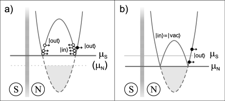
Figure 1: Hole Andreev reflection vs two-electron emission: (a) When $\mu_{S}$ is used as the reference chemical potential both in S and N, a typical scattering process at the NS tunneling interface for $eV\equiv\mu_{S}-\mu_{N}>0$ is that of incoming holes with energies between $\mu_{S}$ and $\mu_{S}+eV$ that are most often normally reflected and only rarely Andreev reflected. (b) If, alternatively, $\mu_{N}$ is used to define quasiparticles in N, the many incoming or outgoing holes are viewed as a vacuum of quasiparticles. The outgoing electron generated in a rare Andreev reflection event appears now as a spontaneously emitted electron above $\mu_{S}$. Such an event causes an outgoing hole state to be empty. This is now perceived as the emission of a second electron with energy between $\mu_{N}$ and $\mu_{S}$. Tracking the spin and the momentum component parallel to the interface leads to the picture of two electrons emitted in a spin singlet state with opposite parallel momenta.

In a biased normal-superconductor tunneling interface in which e.g. the superconductor chemical potential is the greatest, one expects current to be dominated by the injection of electron pairs from the superconductor into the normal metal if the voltage difference $V$ and the temperature $T$ are sufficiently low, single-electron tunneling being forbidden by the energy required to break a Cooper pair. Specifically, one expects two-electron tunneling to dominate if $k_{B}T,eV\ll\Delta$, where $\Delta$ is the zero-temperature superconductor gap. Simple and unquestionable as this picture is, it is not clear how it can be quantitatively described within the popular Bogoliubov - de Gennes (BdG) quasiparticle scattering picture blonder82 ; degennes66 ; beenakker95 . While it leaves the BCS state unchanged, the emission of two electrons into the normal metal involves the creation of two quasiparticles, something that is not possible within the standard BdG formalism, where the quasiparticle number is a good quantum number and the quasiparticle scattering matrix is thus unitary. The conservation of quasiparticle current is a consequence of the implicit assumption contained in the conventional BdG scheme that the reference chemical potential used to identify quasiparticles in the normal metal is the superconductor chemical potential $\mu_{S}$. However, as shown below, one does not need to be constrained by such a choice.

In the mean field description of inhomogeneous superconductivity provided by the BdG formalism, the Hamiltonian is given by

$$H=E_{0}+\sum_{n\sigma}\gamma^{\dagger}_{n\sigma}\gamma_{n\sigma},$$ (1)

where $E_{0}$ is the condensate energy and $\gamma^{\dagger}_{n\sigma}$ creates a quasiparticle of energy $\varepsilon_{n}$, spin quantum number $\sigma$ and wave function $[u_{n}({\bf r}),v_{n}({\bf r})]$ satisfying the BdG equations

$$\left[\begin{array}[]{cc}H_{0}-\mu_{S}&\Delta\\ \Delta^{*}&-H_{0}^{*}+\mu_{S}\end{array}\right]\left[\begin{array}[]{c}u_{n}\\ v_{n}\end{array}\right]=\varepsilon_{n}\left[\begin{array}[]{c}u_{n}\\ v_{n}\end{array}\right],$$ (8)

where $H_{0}=-\hbar^{2}\nabla^{2}/2m+U$ is the one-electron Hamiltonian. In the standard convention one adopts solutions such that $\varepsilon_{n}-\mu_{S}>0$. However, a fundamental property of the BdG equations degennes66 ; sanc95 ; sanc97 is that, for every quasiparticle $n,\sigma$ of energy $\varepsilon_{n}>\mu_{S}$, there exists another solution $n^{\prime},\sigma^{\prime}$ with spin $\sigma^{\prime}=-\sigma$, energy $\varepsilon_{n^{\prime}}=-\varepsilon_{n}+2\mu_{S}<\mu_{S}$ and wavefunction $(u_{n^{\prime}},v_{n^{\prime}})=(-v_{n}^{*},u_{n}^{*})$. These two solutions are not independent, since creating quasiparticle $n,\sigma$ is equivalent to destroying quasiparticle $n^{\prime},-\sigma$ sanc97 . More specifically, $\gamma^{\dagger}_{n\downarrow}=\gamma_{n^{\prime}\uparrow}$, and $\gamma_{n\uparrow}=-\gamma^{\dagger}_{n^{\prime}\downarrow}$.

In the case of a normal metal, where quasiparticles are pure electron or pure holes, the above property implies that creation of a quasiparticle of energy $\varepsilon_{n}>\mu_{S}$ and wave function $(0,v_{n})$ (i.e. a pure hole) corresponds to the destruction of a quasiparticle of energy $\varepsilon_{n}^{\prime}=2\mu_{S}-\varepsilon_{n}<\mu_{S}$ and wave function $(-v_{n}^{*},0)$ (i.e. a pure electron). If $v_{n}({\bf r})\sim\exp(i{\bf k}_{h}\cdot{\bf r})$, the existence of a hole of momentum ${\bf k}_{h}$, with $k_{h}<k_{F}$, and energy $\varepsilon>\mu_{S}$ corresponds to the absence of an electron in the state of wave function $v_{n}^{*}({\bf r})\sim\exp(-i{\bf k}_{h}\cdot{\bf r})$ with energy $\varepsilon^{\prime}=2\mu_{S}-\varepsilon<\mu_{S}$.

In a biased NS tunneling structure, the normal metal has a different chemical potential $\mu_{N}=\mu_{S}-eV$. Without loss of generality, we may assume $\mu_{N}<\mu_{S}$. If we release ourselves from the standard BdG constraint of using $\mu_{S}$ as the reference chemical potential even on the normal side, a clearer picture is likely to emerge. We may decide that, in the energy range $\mu_{N}<\varepsilon^{\prime}<\mu_{S}$, we switch to the opposited convention for the identification and labelling quasiparticles. In other words, we decide to use $\mu_{N}$ as the reference chemical potential. Translated to the example of the previous paragraph, we pass to view the occupation of the hole-type quasiparticle state of wave function $(0,v_{n})$ and energy $\varepsilon>\mu_{S}$ as the emptiness of the electron-type quasiparticle state of wave function $(-v_{n}^{*},0)$ and energy $\varepsilon^{\prime}<\mu_{S}$. Conversely, the absence of quasiparticles in $(0,v_{n})$ is now viewed as the occupation of $(-v_{n}^{*},0)$, i.e. as the existence of an electron with wave function $-v_{n}^{*}({\bf r})$ and energy $\varepsilon^{\prime}$ between $\mu_{N}$ and $\mu_{S}$.

The consequences that this change of paradigm has on the way we view transport through an NS interface can be more clearly appreciated in Fig. 1. In the standard BdG picture represented in Fig. 1(a), with $\mu_{S}$ as the reference chemical potential, the “in” state is that of many holes impinging on the NS interface from the N side, with energies between $\mu_{S}$ and $\mu_{S}+eV$. Since ours is a tunneling structure, normal reflection is the dominant scattering channel and only one hole is Andreev reflected as an electron (quasiparticle transmission is precluded at sufficiently low temperatures and voltages). Thus the “out” state is that of many holes and only one electron moving away from the surface, all with energies also between $\mu_{S}$ and $\mu_{S}+eV$, since quasiparticle scattering is elastic. Given the unitary character of quasiparticle scattering in the BdG formalism, the existence of an outgoing electron requires the outgoing hole quasiparticle state at the same energy to be empty, due to the incoming hole that failed to be normally reflected. The absence of such an outgoing hole is clearly shown in Fig. 1(a).

If we now shift to $\mu_{N}$ as the reference chemical potential, the picture is somewhat different. The many impinging holes on the surfaces are now viewed as the absence of quasiparticles, i.e. the “in” state is the vacuum of quasiparticles. The one electron that emerged from a rare Andreev process continues to be viewed as an occupied electron state, shown above $\mu_{S}$ in Fig. 1(b). The many outgoing holes of the BdG picture are again viewed as an absence of quasiparticles. The second outgoing electron that is needed to complete the picture of two-electron emission corresponds to the empty outgoing hole state of the BdG picture which originates from the hole that failed to be normally (and thus specularly) reflected. It is shown in Fig. 1(b) with energy between $\mu_{N}$ and $\mu_{S}$. As is known from the theory of quasiparticle Andreev reflection, the outgoing electron of Fig. 1(a) follows the reverse path of the incident hole (conjugate reflection). Therefore the two electrons in Fig. 1(b) have momenta with opposite parallel (to the interface) components and the same perpendicular component, i.e. they leave the superconductor forming a V centered around the axis normal to the interface. Inclusion of the spin quantum number completes the picture of two electrons emitted into the normal metal in an entangled spin singlet state.

In summary, we have rigorously established the equivalence between the pictures of Andreev reflection and two-electron emission, noting that they emerge from different choices of the chemical potential to which quasiparticles in the normal metal are referred, $\mu_{S}$ in the standard BdG picture, and $\mu_{N}$ in the scenario which contemplates the spontaneous emission of two electrons. For simplicity, and because it better fits our present need, we have focussed on the case of a tunneling structure. However, the essence of our argument is of general validity. Here we just note that, in the opposite case of a transmissive NS interface blonder82 ; kummel69 , the same argument applies if, exchanging roles, Andreev reflection passes to be the rule while normal reflection becomes the exception. In that case, charge accumulation and its accompanying potential drop, which are generated by normal reflection sols99 , will be essentially nonexistent.

Upon completion of this work, we have learned that the need to change the normal metal vacuum to describe hole Andreev reflection as electron emission has also been noted in Ref. samu03 .

III Formulation of the problem

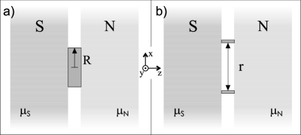
Figure 2: Schematic lateral view of the NS tunneling structures studied in this paper: (a) circular interface of arbitrary radius $R$ and (b) interface made of two small holes at a distance $r$ from each other. The rest of the NS interface is assumed to be opaque.

As has been said, an extensive body of literature has been written on the various aspects of electron transport through a normal-superconductor interface andreev64 ; degennes66 ; griffin70 ; blonder82 ; byers95 ; torres99 ; recher01 ; falci01 ; lesovik01 ; recher02 ; chtc02 ; feinberg03 ; recher03 ; lambert91 ; beenakker92 ; kupka94 ; beenakker95 ; levy95 ; sanc95 ; tinkham96 ; kupka97 ; sanc97 ; sols99 ; nakano94 . Generally those works have focussed on the case of broad interfaces or point contacts beenakker95 ; levy95 . Our goal here is to analyze the current of spin entangled Cooper pairs from a BCS bulk superconductor into a bulk normal metal through an arbitrarily shaped insulating junction in the tunnel limit. Apart from the desire to explore novel types of NS structures, we are also motivated by the need to investigate in depth the two-electron emission picture, which is likely to be useful in the design of quantum communication devices. We wish to consider explicitly geometries of the sort depicted in Fig. 2, i.e. a 2D planar interface of arbitrary radius $R$, presented in Fig. 2(a), and two small orifices separated by a distance $r$, shown in Fig. 2(b). It is assumed that, outside the designed region, the interface is opaque to the flow of electrons. For simplicity, both the normal and the superconducting electrodes are taken to be ballistic. An advantage of the tunneling regime is that the proximity effect may be neglected, i.e. we assume that the gap function drops sharply at the NS interface and that self-consistency in the gap may be safely neglected sanc97 . Another benefit is that we deal at most with two chemical potentials, since the low scale of tunneling currents guarantees that the normal metal is close to equilibrium sols99 and that no phase slips develop within the superconductor sanc01 . Inelastic processes at the interface will also be ignored kirtley92 .

We are interested in a conventional (s-wave) superconductor because it may act as a natural source of spin-entangled electrons, since its electrons form Cooper pairs with singlet spin wave functions and may be injected into a normal metal. The superconductor, which is held at a chemical potential $\mu_{S}$, is weakly coupled by a tunnel barrier to a normal metal which is held at $\mu_{N}$. By applying a bias voltage $V=(\mu_{S}-\mu_{N})/e$ such that $eV>0$, transport of entangled electrons occurs from the superconductor to the normal metal. We focus on the regime $k_{B}T\ll eV\ll\Delta$. Since $\delta\equiv\Delta/E_{F}\sim 10^{-4}$ in a conventional superconductor, rearrangement of the potential barrier due to the voltage bias can be also neglected. However, the effect of a finite, small $\delta$ will often be tracked because pairing correlations (and thus nonlocal entanglement) decays on the scale of the coherence length $\xi_{0}$, which is finite to the extent that $\Delta$ is nonzero. For convenience we assume that the superconductor normal-state properties $(m,k_{F},\rm{etc.})$ are the same as for an ordinary metal.

We will use a tunneling Hamiltonian approach and explicitly consider the emission of two electrons from the superconductor, a viewpoint that will be mandatory in contexts where the late evolution of correlated electron pairs in the normal metal is to be investigated.

IV Three-dimensional tunneling Hamiltonian

The Bardeen model for electron tunneling bardeen61 assumes that a system made up of two bulk metals connected through an insulating oxide layer can be described by the Hamiltonian

$$H=H_{L}+H_{R}+H_{T}\,.$$ (9)

Here $H_{L}$ and $H_{R}$ are the many-body Hamiltonians for the decoupled (i.e. unperturbed) electrodes, the superconductor being on the left and the normal metal on the right. The connection between both electrodes is described by the tunneling term $H_{T}$ (see e.g. Ref. mahan00 ):

$$H_{T}=\sum_{\mathbf{k}\mathbf{q}\sigma}\,T_{\mathbf{k}\mathbf{q}}\,c^{\dagger}_{\mathbf{k}\sigma}\,c_{\mathbf{q}\sigma}+\textrm{H.c.}$$ (10)

Here $c^{\dagger}_{\mathbf{k}\sigma}$ is the creation operator in the normal metal of the single-particle state of orbital quantum number $\mathbf{k}$ and spin $\sigma$, whereas $c_{\mathbf{q}\sigma}$ destroys state $\mathbf{q},\sigma$ in the superconductor and $T_{\mathbf{k}\mathbf{q}}$ is the matrix element connecting both states. We assume a perfect interface defined by a square barrier $U({\bf r},z)=U_{0}\Theta(z+w/2)\Theta(w/2-z)]$ (hereafter r refers to the in-plane coordinate).

If $\chi_{\mathbf{q}}(\mathbf{r},z)$ are the left-side stationary waves for a potential step $U_{L}(\mathbf{r},z)=U_{0}\Theta(z+w/2)$ and $\chi_{\mathbf{k}}(\mathbf{r},z)$ behaves similarly for $U_{R}(\mathbf{r},z)=U_{0}\Theta(w/2-z)$, Bardeen bardeen61 showed

$$T_{\mathbf{k}\mathbf{q}}=\frac{-\hbar^{2}}{2m}\int d\mathbf{r}\,\left[\chi^{\ast}_{\mathbf{k}}(\mathbf{r},z)\frac{\partial}{\partial z}\chi_{\mathbf{q}}(\mathbf{r},z)-\chi_{\mathbf{q}}(\mathbf{r},z)\frac{\partial}{\partial z}\chi^{\ast}_{\mathbf{k}}(\mathbf{r},z)\right]_{z=z_{0}}\,,$$ (11)

where $z_{0}$ lies inside the barrier, i.e. $J_{\mathbf{k}\mathbf{q}}(\mathbf{r},z_{0})\equiv(i/\hbar)T_{\mathbf{k}\mathbf{q}}$ is the matrix element of the $z$ component of the current density operator. Due to charge conservation, $J_{\mathbf{k}\mathbf{q}}$ is independent of the choice of point $z_{0}\in[-w/2,w/2]$. The unperturbed wave functions are of the form

$$\chi_{\mathbf{k}}(\mathbf{r},z)=\frac{e^{i\mathbf{k}_{\parallel}\mathbf{r}}}{\sqrt{A}}\varphi_{k_{z}}(z),$$ (12)

where the exact shape of $\varphi_{k_{z}}(z)$ depends on the barrier height. Thus,

$$T_{\mathbf{k}\mathbf{q}}=\frac{\tau}{\sqrt{\Omega_{L}\Omega_{R}}N(0)}\>\delta(\mathbf{k}_{\parallel}-\mathbf{q}_{\parallel})\,L(k_{z},q_{z})\,.$$ (13)

Hereafter, the volume of each metal $\Omega_{L,R}$ is taken equal to $\Omega=AL$, $A$ being the area of the interface and $L$ the length of each semi-infinite metal. $N(0)$ is the 3D one-spin electronic density of states of the normal metal at the Fermi level: $N(0)=k_{F}^{3}/4\pi^{2}E_{F}$. We define the transparency of the barrier as

$$\tau\equiv 4\sqrt{\frac{E_{F}}{U_{0}}}e^{-p_{0}w}\,,$$ (14)

where $p_{0}\equiv\sqrt{2mU_{0}}/\hbar$. In the particular case $p_{0}w\gg 1$ and $E_{F}\ll U_{0}$, $\tau$ coincides with the probability amplitude that an electron with perpendicular energy $E_{z}=E_{F}$ traverses the barrier. $L(k_{z},q_{z})$ in Eq. (13) captures the dependence of the hopping energy on the $z$ momentum component. Some authors take it as constant, but we shall argue in section IX that its $k_{z}$, $q_{z}$ dependence is crucial for a sound description of 3D transport problems.

For a square barrier, we may define $u\equiv U_{0}/E_{F}$, $\varrho_{z}\equiv q_{z}/k_{F}$, $\kappa_{z}\equiv k_{z}/k_{F}$, and write

$$L(k_{z},q_{z})=k_{z}\,q_{z}\,a(\kappa_{z},\varrho_{z})\,\exp{\{p_{0}w\left[1-a(\kappa_{z},\varrho_{z})\right]\}}\,,$$ (15)

where

$$a(x,y) \equiv [b(x)+b(y)]/2\,,$$ (16)

$$b(x) \equiv \sqrt{1-x^{2}/u}\,.$$ (17)

For high barriers ($u\rightarrow\infty$) we have $a(x)\rightarrow 1$. Then,

$$T_{\mathbf{k}\mathbf{q}}\simeq\frac{\tau}{\Omega N(0)}\,\delta(\mathbf{k}_{\parallel}-\mathbf{q}_{\parallel})\,k_{z}\,q_{z}\,.$$ (18)

If we make $U_{0}\rightarrow\infty$ while keeping the electron transmission probability finite, we are implicitly assuming that the barrier becomes arbitrarily thin ($w\rightarrow 0$), i.e. we are taking it to be of the form $V(z)=H\delta(z)$, as popularized in Ref. blonder82 . On the other hand, since the height of the barrier is judged in relation to the perpendicular energy $E_{z}\leq E_{F}<U_{0}$, it is clear that, given $U_{0}$ and $w$, Eq. (18) becomes correct for sufficiently small $k_{z},q_{z}$. In other words, $T_{\mathbf{k}\mathbf{q}}$ behaves identically for $u\rightarrow\infty$ or $k_{z},q_{z}\rightarrow 0$. As a consequence, such bilinear dependence of $T_{\mathbf{k}\mathbf{q}}$ for sufficiently small $k_{z},q_{z}$ may be expected to hold for arbitrary barrier profiles within the tunneling regime. We note that Eq. (18) differs from the result obtained in Ref. gray65 for the low energy hopping.

IV.1 Validity of the tunneling Hamiltonian model: momentum cutoff

We wish to quantify the idea that a perturbative treatment of Bardeen’s tunneling Hamiltonian is valid only when it involves matrix elements between weakly coupled states bardeen61 ; prange63 .

The transmission probability for a low energy electron incident from the left can be written

$$T(E_{z})=W_{\mathbf{q}}/J_{\mathbf{q}}\,,$$ (19)

where $J_{\mathbf{q}}$ is the current density carried by the incoming component of the stationary wave q, and

$$W_{\mathbf{q}}=\frac{2\pi}{\hbar}\sum_{\mathbf{k}}|T_{\mathbf{k}\mathbf{q}}|^{2}\delta(E_{\mathbf{k}}-E_{\mathbf{q}})\,$$ (20)

is the tunneling rate. Using Eqs. (13) and (15), Bardeen’s theory yields

$$T(E_{z})=16\frac{E_{z}}{U_{0}}\left(1-\frac{E_{z}}{U_{0}}\right)e^{-2p_{z}w}\,,$$ (21)

where $p_{z}=\sqrt{2m(U_{0}-E_{z})}/\hbar$. On the other hand, an exact calculation galindo90 recovers the tunneling result (21) for $E_{z}<U_{0}$ com-duke ; duke69 if we make the approximation

$$\sinh(p_{z}w)\approx\cosh(p_{z}w)\approx e^{p_{z}w}/2\,.$$ (22)

Thus we adopt as a criterion of the validity of Bardeen’s approximation that Eq. (22) holds, which from (21), implies $T(E_{F})\ll 1$. This defines an upper energy cutoff $E_{c}$ in the various sums over electron states, which is the maximum energy for which the approximation (22) is valid. For the square barrier, $E_{c}\simeq U_{0}-\hbar^{2}/2mw^{2}$.

For processes described by amplitudes which are first order in $H_{T}$, and as long as $U_{0}$ is high enough compared to $E_{F}$ to fulfill condition (22) for all relevant $E_{z}$, all electron momenta lie within the applicability of the tunnel limit and we may use the tunneling Hamiltonian safely. That is the case of the tunnel current through a NN interface or the quasiparticle tunnel current through a NS interface.

The situation is different for transport through a NS interface, since it requires the coherent tunneling of two electrons. Then, the leading contribution to the tunneling amplitude is quadratic in $H_{T}$ and the final transmission probability is sensitive to the existence of intermediate virtual states where only one electron has tunneled and a quasiparticle above the gap has been created in the superconductor. Unlike the weighting factors of the initial and final states, which are controlled by the Fermi distribution function, the contribution of the virtual intermediate states decays slowly with energy and the cutoff $E_{c}$ may be reached. In section V we show that there are two cases where the cutoff can be safely neglected, namely, the limit of high barrier ($u\gg 1$) and the limit of small gap ($\delta\ll 1$).

IV.2 Tunneling Hamiltonian in real space

One of our main goals is to investigate transport through tunneling interfaces of arbitrary shape chen90 that are otherwise uniform. For that purpose we need a reliable tunneling Hamiltonian expressed in real space. Our strategy will be to rewrite Eq. (10) as an integral over the infinite interface and postulate that a similar Hamiltonian, this time with the integral restricted to the desired region, applies to tunneling through the finite-size interface. The discontinuity between the weakly transparent interface and the completely opaque region causes some additional scattering in the electronic wave functions that enter the exact matrix element. However, this effect should be negligible in the tunneling limit. In fact, we provide in Appendix A an independent derivation of the continuum results shown in this section which starts from a discrete tight-binding Hamiltonian.

Thus, in (10) we introduce the transformations

$$c^{\dagger}_{\mathbf{k}\sigma}=\int_{A}d\mathbf{r}\int\!\!dz\;\chi_{\mathbf{k}}(\mathbf{r},z)\>\psi^{\dagger}_{N}(\mathbf{r},z;\sigma)$$ (23)

$$c_{\mathbf{q}\sigma}=\int_{A}d\mathbf{r}\int dz\;\chi^{*}_{\mathbf{q}}(\mathbf{r},z)\>\psi_{S}(\mathbf{r},z;\sigma)$$ (24)

where the wave functions $\chi_{\mathbf{q}}$ and $\chi_{\mathbf{k}}$ are, respectively, solutions of $H_{L}$ and $H_{R}$ and are given in (12). $\psi^{\dagger}_{N}(\mathbf{r},z;\sigma)$ and $\psi_{S}(\mathbf{r},z;\sigma)$ are the field operator in the normal and superconducting metals.

Invoking Eq. (13) and the completeness of plane waves in the $x,y$ plane [which yields a term $\delta(\mathbf{r}-\mathbf{r}^{\prime})$], we obtain

$$H_{T}=\sum_{\sigma}\frac{\tau}{4\pi^{2}N(0)}\int_{A}d\mathbf{r}\int dz^{\prime}\int dz\>\widetilde{L}(z,z^{\prime})\>\psi^{\dagger}_{N}(\mathbf{r},z;\sigma)\,\psi_{S}(\mathbf{r},z^{\prime};\sigma)+\textrm{H.c.}\,,$$ (25)

where

$$\widetilde{L}(z,z^{\prime})=\frac{1}{L_{z}}{\sum_{k_{z},q_{z}>0}}\varphi_{k_{z}}\!(z)\,\varphi^{*}_{q_{z}}\!(z^{\prime})\,L(k_{z},q_{z})\,.$$ (26)

Since the initial Hamiltonian (10) connects states which overlap in a finite region below and near the barrier, it is logical that the real space Hamiltonian (25) is non-local in the $z$-coordinate. An interesting limit is that of a high and (to keep transmission finite) thin barrier, i.e. the delta barrier limit. Then, the perpendicular wave functions can be precisely written

$$\varphi_{k_{z}}\!(z)=\sqrt{2/L}\sin(k_{z}z),\;\;z\geq 0$$ (27)

and similarly for the left electrode. We introduce such wave functions in Eq. (26) and invoke the identity (hereafter $L\rightarrow\infty$)

$$\frac{1}{L}\sum_{k_{z}>0}k_{z}\sin(k_{z}z)=-\delta^{\prime}(z),$$ (28)

where the volume per orbital in $k_{z}$-space is $\pi/L$. Then, to leading order in $u^{-1}\ll 1$, Eq. (25) yields

$$H_{T}=\sum_{\sigma}\frac{\tau}{8\pi^{2}N(0)}\int_{A}\!d\mathbf{r}\,\left.\frac{\partial\psi^{\dagger}_{N}(\mathbf{r},z;\sigma)}{\partial z}\right|_{z\rightarrow 0^{+}}\left.\frac{\partial\psi_{S}(\mathbf{r},z^{\prime};\sigma)}{\partial z^{\prime}}\right|_{z^{\prime}\rightarrow 0^{-}}+\textrm{H.c.}$$ (29)

If we replace the thermodynamic area $A$ by a specific finite area, the real space Hamiltonian (29) can be used to describe tunneling through interfaces of arbitrary shape. As we have said, in Appendix A we provide an alternative derivation which makes Eq. (29) appear as the natural continuum limit of the hopping Hamiltonian in a regularized tight-binding representation. We note that the tunneling Hamiltonian (29) may also be obtained if the r.h.s. of Eq. (27) is replaced by a plane wave representation.

¿From Eq. (29) we conclude that apparently reasonable choices of local tunneling Hamiltonian such as those $\propto\int\psi_{S}^{\dagger}\psi_{N}$ lead to unphysical results in 3D. This point will be discussed in depth in section IX.

To describe tunneling in real space, rather than starting from Hamiltonian (25), or its limiting version (29), it is more convenient in practice to go back to Eq. (13) and make the replacement $\delta(\mathbf{k}_{\parallel}-\mathbf{q}_{\parallel})\rightarrow(2\pi)^{-2}\int_{A}d\mathbf{r}\,e^{i(\mathbf{k}_{\parallel}-\mathbf{q}_{\parallel})\cdot\mathbf{r}}$, with $A$ finite. Then Eqs. (25) and (26) may equivalently be written

$$H_{T}\!=\!\sum_{\mathbf{k}\mathbf{q}\sigma}\frac{\tau(2\pi)^{-2}}{N(0)\Omega}\int_{A}\!d\mathbf{r}\,e^{i(\mathbf{k}_{\parallel}-\mathbf{q}_{\parallel})\cdot\mathbf{r}}L(k_{z},q_{z})c^{\dagger}_{\mathbf{k}\sigma}\,c_{\mathbf{q}\sigma}+\textrm{H.c.}$$ (30)

If we make $L(k_{z},q_{z})=k_{z}q_{z}$, it is easy to prove that (30) becomes (29).

V Perturbative calculation of the stationary current

Following Ref. recher01 , we write the stationary electron current from the superconductor to the normal metal as

$$I_{\rm NS}=2e\sum\limits_{if}W_{fi}\,\rho_{i}\,,$$ (31)

where $W_{fi}$ is the transition rate at which two electrons tunnel from the superconductor into the normal metal, and $\rho_{i}$ is the stationary distribution accounting for a chemical potential difference $eV$ between the two electrodes. We calculate the transition rate with a $T$-matrix approach merzbacher98 ,

$$W_{fi}=\frac{2\pi}{\hbar}\,|\langle f|\,\hat{T}(\varepsilon_{i})\,|i\rangle|^{2}\,\delta(\varepsilon_{f}-\varepsilon_{i})\,.$$ (32)

The $T$-matrix can be written as a power series in the tunnel Hamiltonian $H_{T}$,

$$\hat{T}(\varepsilon)=H_{T}+H_{T}\sum_{n=1}^{\infty}[G_{0}(\varepsilon)H_{T}]^{n}\,$$ (33)

where $G_{0}(\varepsilon)=(\varepsilon-H_{0}+i0^{+})^{-1}$ is the retarded Green function for the decoupled system.

At zero temperature the initial state is $|i\rangle=|\textrm{F}\rangle\otimes|\textrm{BCS}\rangle$, where $|\textrm{F}\rangle$ is the filled Fermi sea ground state of the normal metal and $|\textrm{BCS}\rangle$ is the BCS ground state of the superconductor. The state $|i\rangle$ is the vacuum of quasiparticles if these are referred to $\mu_{S}$ in the superconductor and to $\mu_{N}=\mu_{S}-eV$ in the normal metal (see section II). In the final state

$$|f\rangle=\frac{1}{\sqrt{2}}(c^{\dagger}_{\mathbf{k}_{1}\uparrow}c^{\dagger}_{\mathbf{k}_{2}\downarrow}-c^{\dagger}_{\mathbf{k}_{1}\downarrow}c^{\dagger}_{\mathbf{k}_{2}\uparrow})|i\rangle\,,$$ (34)

i.e. the superconductor remains unperturbed within the BCS description, since an entire Cooper pair has been removed, and two singlet-correlated electrons hover above the normal Fermi sea comm-Fermi . In the ensuing discussion we take $\varepsilon_{i}=2\mu_{S}\equiv 0$.

Since we wish to focus on the regime $k_{B}T\ll eV\ll\Delta$, single electron emission is forbidden due to energy conservation, because it requires the breaking of a Cooper pair. Therefore, to leading order in $H_{T}$, we may approximate

$$\hat{T}(0)\approx T^{{}^{\prime\prime}}\!\equiv H_{T}\,G_{0}\,H_{T}\,$$ (35)

and so we write

$$\langle f|\hat{T}(0)|i\rangle=\frac{1}{\sqrt{2}}\,\langle(c_{\mathbf{k}_{2}\downarrow}c_{\mathbf{k}_{1}\uparrow}-c_{\mathbf{k}_{2}\uparrow}c_{\mathbf{k}_{1}\downarrow})\,T^{{}^{\prime\prime}}\rangle\,.$$ (36)

We insert a complete set of single-quasiparticle (virtual) states, i.e. $1\!\!1=\sum_{\mathbf{k}\mathbf{q}\sigma\sigma^{\prime}}\gamma^{\dagger}_{\mathbf{q}\sigma}c^{\dagger}_{\mathbf{k}\sigma^{\prime}}|i\rangle\langle i|c_{\mathbf{k}\sigma^{\prime}}\gamma_{\mathbf{q}\sigma}$, between the two $H_{T}$ in (35) and we use the fact that the resulting energy denominator $|i0^{+}-\xi_{\mathbf{k}}-E_{\mathbf{q}}|\approx|E_{\mathbf{q}}|$, since $\xi_{\mathbf{k}}\equiv\hbar^{2}k^{2}/2m-\mu_{N}\rightarrow 0$ when $eV\rightarrow 0$. To see this, one must note that the energy conservation implies $\varepsilon_{f}=\varepsilon_{i}$; therefore, $\varepsilon_{f}=\xi_{\mathbf{k}_{1}}+\xi_{\mathbf{k}_{2}}-2eV=2\mu_{S}=0$. Thus, when $eV\rightarrow 0$, one may write $\xi_{\mathbf{k}_{1}}\approx-\xi_{\mathbf{k}_{2}}\approx 0$ . We also make use of $u_{\mathbf{q}}v_{\mathbf{q}}=u_{-\mathbf{q}}v_{-\mathbf{q}}$. Finally, we get

$$\langle f|\hat{T}(0)|i\rangle=$$

$$~{}~{}=2\sqrt{2}\langle c_{\mathbf{k}_{2}\uparrow}c^{\dagger}_{\mathbf{k}_{2}\uparrow}c_{\mathbf{k}_{1}\downarrow}c^{\dagger}_{\mathbf{k}_{1}\downarrow}\rangle{\sum_{\mathbf{q}}}\frac{\langle c_{\mathbf{q}\uparrow}c_{\mathbf{-q}\downarrow}\rangle}{E_{\mathbf{q}}}T_{\mathbf{k}_{1}\mathbf{q}}T_{\mathbf{k}_{2},\mathbf{-q}}~{}~{}~{}~{}~{}~{}$$ (37)

where $E_{\mathbf{q}}=[(\hbar^{2}/2m)^{2}(q^{2}-k_{F}^{2})^{2}+\Delta^{2}]^{1/2}$ is the quasiparticle energy and $F_{\mathbf{q}}\equiv\langle c_{\mathbf{q}\uparrow}c_{\mathbf{-q}\downarrow}\rangle$ is the condensation amplitude in the state $\mathbf{q}$ degennes66 .

At zero temperature we have $F_{\mathbf{q}}=\Delta/2E_{\mathbf{q}}$. Thus, in the summation of Eq. (V), the contribution of high energy virtual states is weighted by the Lorentzian $F_{\mathbf{q}}/E_{\mathbf{q}}$, of width $\Delta$ and centered around $E_{F}$. We already mentioned in the previous section the need for a high-energy cutoff $E_{c}$ to prevent the inclusion of states for which the tunneling approximation is not valid. However, in the limit $\Delta/E_{F}\rightarrow 0$, the Lorentzian distribution becomes a delta function and the results are independent of the cutoff, which can be safely taken to infinity. A similar situation is found in the limit $U_{0}\gg E_{F}$, for which the sum in Eq. (V) converges before reaching the energy $E_{c}$ above which Bardeen’s approximation is no longer valid. In any of these two limits ($\Delta/E_{F},E_{F}/U_{0}\ll 1)$, it is correct to take $E_{c}\rightarrow\infty$.

VI Total current and angular distribution through a broad interface

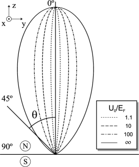
Figure 3: Angular dependence of the normalized tunnel current ranging from $U_{0}/E_{F}\rightarrow\infty$ for the outer ($\cos^{5}\theta$) curve to $U_{0}/E_{F}=1.1$ for the inner one. Finite barriers have a width $w=5\lambda_{F}$. Observe how the angular distribution focalizes around the perpendicular direction as the barrier hight decreases.

The current through a NS junction is most easily calculated when the interface section is much bigger than $\lambda_{F}$. We shall refer to it as the broad interface or thermodynamic limit. Its detailed understanding is of interest for later reference in the investigation of finite size interfaces. For $k_{B}T\ll eV\ll\Delta$, the set of equations in the previous section yields

$$I_{\rm{NS}}=I_{V}\frac{\tau^{4}}{2}\int_{0}^{\pi/2}\!d\theta\,\sin\!\theta\,g(\theta)\,,$$ (38)

where $g(\theta)$ is the angular distribution ($\theta$ being the angle between the outgoing electron momentum and the direction normal to the interface) and

$$I_{V}\equiv\ \frac{1}{2}\,e^{2}\,VN(0)\,v_{F}\,A\,=J_{V}A\ ,$$ (39)

with $V$ the applied voltage, $A$ the interface area, and $v_{F}$ the Fermi velocity. Eq. (39) may be written as $I_{V}=(2e^{2}/h)NV$, where $N=Ak_{F}^{2}/4\pi$ is the number of transverse channels that fit in an interface of area $A$. Thus, $I_{V}$ can be interpreted as the current that would flow through a transmissive [$T(E_{z})=1$ for all $E_{z}$] normal-normal interface with the same area and subject to the same voltage bias. The $\tau^{4}$ dependence of $I_{\rm NS}$ reflects the simultaneous tunneling of two electrons.

Using the previous definition $\varrho_{z}\equiv q_{z}/k_{F}$, the angular distribution for the current through an arbitrary square barrier is comm-morten99 ; mortensen99

$$g(\theta)=2\cos^{3}\theta\,e^{2p_{0}w[1-b(\cos\theta)]}\left[\frac{2}{\pi}\int_{0}^{\varrho_{c}}\!\!\!d\varrho_{z}\>\frac{\delta}{(\varrho_{z}^{2}-\cos^{2}\theta)^{2}+\delta^{2}}\>\varrho_{z}^{2}\>\left[a(\varrho_{z},\cos\theta)\right]^{2}\>e^{p_{0}w[1-b(\varrho_{z})]}\right]^{2}\,,$$

where $\varrho_{c}=\sqrt{E_{c}/E_{F}}$ is the cutoff and the functions $a$ and $b$ were defined in Eqs. (16) and (17).

For $\delta\rightarrow 0$, we have

$$\lim_{\delta\rightarrow 0}\int_{0}^{\varrho_{c}}\!\!\!d\varrho\,\frac{\delta}{(\varrho^{2}\!-\!x^{2})^{2}\!+\delta^{2}}\;\varrho\,f(\varrho)=\frac{\pi}{2}\,f(x)\,,$$ (41)

if, as is the case, $\varrho_{c}>1\geq|x|$. Therefore, in the limit $\delta\rightarrow 0$, Eq. (VI) yields

$$g(\theta)=2\,e^{4p_{0}w[1-b(\cos\!\theta)]}[b(\cos\!\theta)]^{4}\cos^{5}\!\theta\,.$$ (42)

For large barriers ($u\gg 1$) and finite $\delta$ we find (with $\varrho_{c}\rightarrow\infty$)

$$g(\theta) = \cos^{5}\!\theta+\cos^{3}\!\theta\sqrt{\cos^{4}\!\theta+\delta^{2}}$$ (43)

$$= 2\cos^{5}\theta\left[1+\mathcal{O}(\delta^{2})\right].$$ (44)

Combining Eqs. (38) and (43), we obtain for the total current

$$I_{\rm{NS}} = \frac{1}{12}I_{V}\tau^{4}\left[1+(1+\delta^{2})^{3/2}-\delta^{3}\right]$$ (45)

$$= \frac{1}{6}I_{V}\tau^{4}\left[1+\mathcal{O}(\delta^{2})\right].$$ (46)

However, if the cutoff $\varrho_{c}$ remains finite, Eq. (46) must be replaced by

$$I_{\rm{NS}}=\frac{1}{6}I_{V}\tau^{4}\left[1-\frac{24}{5\pi}\frac{\delta}{\varrho_{c}}+\mathcal{O}(\delta^{2})\right],$$ (47)

i.e. a finite cutoff qualitatively affects the leading low-$\delta$ dependence of $I_{\rm NS}$.

The underlying physics goes as follows. The product of hopping matrix elements appearing in (V) satisfies

$$T^{\ast}_{\mathbf{k_{1}}\mathbf{q}}T^{\ast}_{\mathbf{k_{2}},\mathbf{-q}}\propto k_{1z}\>k_{2z}\>q_{z}^{2}\>\delta(\mathbf{k}_{1\parallel}+\mathbf{k}_{2\parallel})\delta(\mathbf{k}_{1\parallel}-\mathbf{q}_{\parallel})\,.$$ (48)

Thus, when crossing the barrier, electrons forming a Cooper pair of momenta ($\mathbf{q},-\mathbf{q}$) undergo the following process: Their opposite interface-parallel momenta are conserved ($\mathbf{k}_{1\parallel}=\mathbf{q}_{\parallel}$ and $\mathbf{k}_{2\parallel}=-\mathbf{q}_{\parallel}$). By contrast, one of their perpendicular momentum components (more specifically, the negative one pointing away from the interface) is reversed so that both electrons enter the normal metal with perpendicular momenta $k_{1z},k_{2z}>0$. In the limit of $eV\rightarrow 0$ the modulus difference between $k_{1z}$ and $k_{1z}$ is negligible. This means that the electron current through a broad interface will propagate into the normal lead in the form of two rays which are symmetric with respect to the direction normal to the interface. Due to axial symmetry, $g$ is only a function of the zenithal angle $\theta\in[0,\pi/2]$.

The normalized angular distributions for several barrier heights are depicted in Fig. 3 in the limit $\delta\rightarrow 0$. The lowest barrier which we have considered has $u=1.1$. This means that, for a typical value of $E_{F}=5$ eV, the difference between the height of the barrier and the Fermi energy is $0.5$ eV, i.e. large enough to ensure that the junction operates in the tunneling regime. In Fig. 3, finite-height barriers are taken to have a width $w=5\lambda_{F}$. For large $U_{0}$ we reproduce the analytical $\cos^{5}\theta$ behavior given in Eq. (44). As the barrier height decreases, the angular distribution becomes more focussed in the forward direction because transmission is more sensitive to the perpendicular energy. Thus the relative fraction of Fermi surface electrons crossing the interface with $E_{z}$ close to the highest value $E_{F}$ increases. That majority of transmitted electrons have low parallel momenta and, accordingly, a characteristic parallel wave length much larger than $\lambda_{F}$. We will see later that this perpendicular energy selection bears consequences on the length scale characterizing the dependence of the total current on the radius of the interface.

In general, knowledge of the current angular distribution is physically relevant, as one is ultimately interested in directionally separating the pair of entangled electron beams for eventual quantum information processing. To acquire a more complete picture, we may compare the previous results with the case of a NN interface. In that case the total tunnel current is

$$I_{\rm{NN}}=I_{V}\tau^{2}\int_{0}^{\pi/2}\!d\theta\,\sin\!\theta\,g(\theta)\,,$$ (49)

where $I_{V}$ is given in Eq. (39) and, for large $u$,

$$g(\theta)=2\cos^{3}\theta\,.$$ (50)

Thus we see that electron transport through a tunneling NN interface also exhibits focussing which is however less sharp than in the NS case [see Eq. (44)]. The term $\tau^{2}$ in Eq. (50) reflects the dominance of single-electron tunneling at the NN interface. Finally, we may compare Eqs. (44) and (50) with the $\cos\theta$ distribution law exhibited by electron current in the bulk of a disordered wire comm1 .

VI.1 Connection with the multi-mode picture

We could have derived the angular distributions in Eqs. (38), (44), (49) and (50) following the scattering theory of conduction in normal landauer57 and normal-superconducting beenakker92 multichannel wires. For an NN interface we can write the relation between conductance and transmission probabilities at the Fermi energy as

$$G_{\rm NN}=\frac{2e^{2}}{h}\sum_{n=1}^{N}A_{n}=\frac{2e^{2}}{h}\sum_{n=1}^{N}T_{n}\,,$$ (51)

where $A_{n}$ $(n=1,2,...N)$ are the eigenvalues of the transmission matrix $tt^{+}$ at the Fermi energy and $T_{n}\equiv\sum_{m=1}^{N}|t_{nm}|^{2}$ are the modal transmission probabilities at the same energy beenakker95 , which is what we calculate. The exchangeability of $\sum_{n}A_{n}$ and $\sum_{n}T_{n}$ reflects the invariance of the trace comm-trace . Now consider the transmission probability through a square barrier given in Eq. (21). We replace $T_{n}\rightarrow T(E_{z})$. For $E_{z}/U_{0}\ll 1$, we have $T(E_{z})\propto E_{z}\propto\cos^{2}\theta$. Moreover, the sum over transverse modes can be replaced by an integration over the zenithal angle, $\sum_{n}\rightarrow{\rm cnst.}\times\int_{0}^{\pi/2}d\theta\sin\theta\cos\theta$. Altogether, the angular distribution follows the $\cos^{3}\theta$ law expressed in Eq. (50).

A similar line of argument can be followed for the Andreev current through a NS interface, whose conductance is given by

$$G_{\rm NS}=\frac{2e^{2}}{h}\sum_{n=1}^{N}\frac{2A_{n}^{2}}{(2-A_{n})^{2}}\,.$$ (52)

As noted in Ref. beenakker95 , the equivalence invoked in Eq. (51) is no longer applicable in Eq. (52) because of its nonlinearity. Nevertheless, in the tunneling limit one has $A_{n}\ll 1$ and $G_{\rm NS}$ can thus be approximated as

$$G_{\rm NS}\simeq\frac{2e^{2}}{h}\sum_{n=1}^{N}\frac{A_{n}^{2}}{2}=\frac{2e^{2}}{h}\sum_{n=1}^{N}\frac{T_{n}^{2}}{2}\,,$$ (53)

where the second equality is possible because $\sum_{n}A_{n}^{2}={\rm{Tr}}(tt^{+})^{2}$. Arguing as we did for the NN conductance, it follows that $g(\theta)\propto\cos^{5}\theta$, which confirms Eq. (44). We note here that, in Refs. beenakker92 ; beenakker95 , the Andreev approximation was made whereby all the momenta involved are assumed to be equal to $k_{F}$. In our language, this corresponds to taking $\delta\rightarrow 0$ in Eq. (VI) and thereafter.

Finally, comparison of Eqs. (51) and (53) also illuminates the contrast between the factor $\tau^{4}/2$ in Eq. (38) and the factor $\tau^{2}$ in Eq. (49).

VI.2 Universal relation between NN and NS tunneling conductances

In the case of a normal interface with high barrier, the total current can be integrated to yield

$$I_{\rm{NN}}=\frac{I_{V}\tau^{2}}{2}=\left(\frac{2e^{2}}{h}\right)\frac{\tau^{2}}{2}NV\,.$$ (54)

Thus $\tau^{2}/2$ is the average transmission per channel comm-BTK ; sharvin65 . In one dimension ($N=1$) one has $I_{\rm NN}=(2e^{2}/h)V\tau^{2}$. Eqs. (39), (45), and (54) suggest the universal relation

$$\frac{I_{V}I_{\rm NS}}{(I_{\rm NN})^{2}}=\frac{G_{V}G_{\rm NS}}{(G_{\rm NN})^{2}}=\frac{2}{3}\,,$$ (55)

where $G_{i}=I_{i}/V$ ($i={\rm V,NS,NN}$). Eq. (55) indicates that knowledge of $G_{\rm NS}$ and $G_{\rm NN}$ may allow us to infer $G_{V}$ and, from (39), the effective area of a tunneling interface.

VI.3 Comparison with the quasiparticle scattering method

Blonder et al. blonder82 studied transport through a one-dimensional NS interface modelled by a delta-barrier one-electron potential [$U(z)=H\delta(z)$] by solving for the quasiparticle scattering amplitudes. If the dimensionless parameter $Z=mH/\hbar^{2}k_{F}$ is employed to characterize the scattering strength of the barrier, the tunneling limit corresponds to $Z\gg 1$, for which they obtained $I_{\rm NS}^{\rm 1D}=I_{V}/Z^{4}$ assuming $k_{B}T\ll eV\ll\Delta\ll E_{F}$ (i.e. a low-transmission regime in which Andreev reflection is the only charge-transmitting channel). Later, Kupka generalized the work of Ref. blonder82 to investigate the sensitivity of Andreev and normal reflection to the thickness of the barrier kupka94 and to the presence of a realistic 3D geometry kupka97 . For the case of a broad interface in the tunneling limit he obtained $I_{\rm NS}^{\rm 3D}=I_{V}/6Z^{4}$. Therefore, Kupka found a result identical to Eq. (46) (to zeroth order in $\delta$) with $\tau$ replaced by $1/Z$. In fact, it is easy to see that, in the case of a delta-barrier with $Z\gg 1$, the transparency defined in section IV is precisely $\tau=1/Z$. Therefore, comparison of Eqs. (44) and (46) with the results of Ref. kupka97 completes the discussion of section II by establishing the quantitative equivalence between the pictures of quasiparticle Andreev reflection and two-electron (or two-hole) emission. We note that, in Refs. blonder82 ; kupka94 ; kupka97 , the Andreev approximation ($\delta\rightarrow 0$) was made.

VII Current through a circular interface of arbitrary radius

In this section we investigate transport through a circular NS tunneling interface of arbitrary radius. The setup is as depicted in Fig. 2(a). To make the discussion more fluent, lengthy mathematical expressions have been transferred to Appendix B, leaving here the presentation of the main results, which include some analytical expressions for the limit of small gap and high barrier.

VII.1 Total current

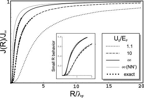
Figure 4: Radial dependence of the normalized NS Andreev tunnel current through a circular interface of radius $R$ for different barrier heights. $J(R)\equiv I(R)/\pi R^{2}$ and $J_{\infty}$ is the current density in the thermodynamic limit. Finite barriers have a width $w=5\lambda_{F}$. Everywhere $\Delta/E_{F}\ll 1$ is taken. Dots correspond to numerically exact results. Solid lines are computed with an approximation described in Appendix B which becomes exact for $R/\lambda_{F}\gg 1$. The inset magnifies results for small $R$.

The most general expression for the current is given in Eq. (B). Below we focus on the limit $\delta,u^{-1}\ll 1$. We find three regimes of interest, depending on the value of $R/\lambda_{F}$.

VII.1.1 Small radius ($R\ll\lambda_{F}$)

This limit is not physically realizable, at least with current materials. However, it is interesting for two reasons. First, it yields a radius dependence that directly reflects the entangled nature of the electron current. Second, it can be used as a unit of current such that, when referred to it, calculated currents have a range of validity that goes well beyond the geometrical model here considered. That permits a direct comparison between different theoretical models and experimental setups.

For $k_{F}R\ll 1$ we obtain

$$I(R)\simeq I_{0}\equiv\frac{2\pi}{6^{4}}J_{V}\tau^{4}k_{F}^{6}R^{8}.$$ (56)

This $R^{8}$ behavior is easy to understand. To compute the current we must square the matrix element between the initial and the final state, i.e. the Cooper pair hopping amplitude. The tunneling of each electron involves an integral over the interface, which for $k_{F}R\ll 1$ contributes a factor $R^{2}$ to the amplitude, regardless of the incident angle. The Cooper pair amplitude becomes $\sim R^{4}$, which leads to the $R^{8}$ behavior for the probability.

It is interesting to compare the $R^{8}$ law here derived with, e.g. the $R^{4}$ behavior of the NN tunnel current ($u\gg 1$), namely,

$$I_{0}\simeq\frac{\pi}{9}J_{V}\tau^{2}k_{F}^{2}R^{4}\,,$$ (57)

or with the $R^{6}$ dependence for the transmission of photons through a circular aperture bethe44 .

Eqs. (56) and Eq. (57) yield the following relation for the narrow interface conductances:

$$G_{\rm NS}=\frac{h}{4e^{2}}G^{2}_{\rm NN}\,\,\,(R\rightarrow 0)\ .$$ (58)

It is important to note that Eq. (58) still applies if both conductances are replaced by their momentum-independent counterparts.

In Fig. 4 we plot the current density as a function of the interface radius. Dots represent the exact calculation taken from Eqs. (90) and (92), which we have been able to evaluate numerically for $u\rightarrow\infty$ (up to $R=1.65\lambda_{F}$) and $u=10$ (up to $R=3\lambda_{F}$), while solid lines are obtained from a large-radius approximation described in Appendix B. For $u=1.1$ convergence problems prevent us from presenting numerically exact results. We find that the small-radius approximation ($\sim R^{8}$) is correct within $1\%$ accuracy up to $R\sim 0.1\lambda_{F}$. Above that value it overestimates the current.

VII.1.2 Intermediate radius ($\lambda_{F}<R<\infty$)

In this region no analytical expression for the current is possible. Above $R\approx 2\lambda_{F}$ even the numerical calculation of Eq. (92) (which presumes $\delta,u^{-1}\ll 1$) is difficult, since for large radii we cannot compute five strongly oscillating nested integrals. A set of two approximations which reduces the number of nested integrals from five to three is discussed in Appendix B and expressed in Eqs. (B) and (95).

In Fig. 4 we plot $I(R)/I(R\rightarrow\infty)$, which is the total current normalized to the thermodynamic limit expression (38) with $A$ in Eq. (39) replaced by $\pi R^{2}$. For finite barriers, $w=5\lambda_{F}$ has been taken. A free parameter has been adjusted to fit the numerically exact result in the region where it is available. As explained in Appendix B, such a scheme is particulary well suited for moderate-to-large radius values. The inset of Fig. 4 shows that, as expected, the approximation fails for small values of $R$, where it yields an $R^{4}$ behavior instead of the correct $R^{8}$ law, thus overestimating the current.

Here we wish to remark that, unlike in the case of a clean NS point contact beenakker92 ; beenakker95 , the radial current dependence shows no structure of steps and plateaus as more channels fit within the area of the interface. This is due the fact that we operate in the tunneling regime, which decreases the height of the possible steps and, more importantly, to the strongly non-adiabatic features of the structure along the $z$-direction.

VII.1.3 Large radius ($R\rightarrow\infty$)

While a numerically exact calculation is already nonfeasible for $R$ a few times $\lambda_{F}$, the approximation described in Appendix B becomes increasingly accurate for large $R$. This allows us to conveniently investigate how the broad interface limit is recovered [see Eqs. (38) and (46)]. Such a limit is characterized by $I(R)$ growing with $R^{2}$, i.e. proportionally to the area, a behavior also shown by the NN conductance. Convergence to the thermodynamic limit is much slower for low barriers than for large barriers. The reason has to do with focussing. The wave length of the characteristic energies $E_{\parallel}=E-E_{z}$ determines the length scale over which the relative phase between distant hopping events varies appreciably. This is the distance over which multiple hopping points (which play the role of multiple “Feynman paths”) cancel destructively for large radius interfaces. As discussed in the previous section, low barriers are more energy selective, making most of the electrons leave with $E_{z}$ close to $E_{F}$ and thus with small $E_{\parallel}$. As a consequence, saturation to the large radius limit is achieved on the scale of many times $\lambda_{F}$. By contrast, high barriers are less energy selective and give a greater relative weight to electrons with low $E_{z}$ and high $E_{\parallel}$. A large fraction of the electrons has a short parallel wave length. This explains why, for high barriers, the large $R$ behavior is reached on a short length scale.

VII.2 Length scales in the thermodynamic limit

It is known that pairing correlations between electrons decay exponentially on the scale of the coherence length $\xi_{0}=\lambda_{F}/\pi^{2}\delta$. This fact is reflected by the exponential factors contained in the integrands of the equations for $I(R)$ in Appendix B. Thus one might expect that the thermodynamic limit relies on such a decay of correlations.

The following argument might seem natural. The double integral over the interface of area $A$ may be viewed as an integral of the two-electron center of mass, which yields a factor $A$, and an integration over the relative coordinate, which is independent of $A$ due to a convergence factor which expresses the loss of pairing correlations. The final current would grow as $I\sim A\xi_{0}^{2}\sim A/\delta^{2}$. However, as discussed in the previous subsection, the thermodynamic limit is achieved on a much shorter scale, namely, the Fermi wave length. If an electron leaves through point ${\bf r}_{1}$ one may wonder what is the contribution to the amplitude stemming from the possibility that the second electron leaves through ${\bf r}_{2}$, eventually integrating over ${\bf r}_{2}$. Eq. (30) suggests that the amplitude for two electrons leaving through ${\bf r}_{1}$ and ${\bf r}_{2}$ will involve the sum of many oscillating terms with different wave lengths, the shortest ones being $\sim\lambda_{F}$. This reflects the interference among the many possible momenta that may be involved in the hopping process. Such an interference leads to an oscillating amplitude which decays fast on the scale of $\lambda_{F}$, rendering the exponentially convergent factor irrelevant. Thus, in the thermodynamic limit the current tends to a well defined value for $\xi_{0}\rightarrow\infty$ ($\delta\rightarrow 0$). In Appendix B we provide a more mathematical discussion of this result.

One may also investigate the first correction for small, finite $\delta$. As indicated in Eqs. (45) and (46), it increases the current. However, in the presence of a finite cutoff ($\varrho_{c}<\infty$), a nonzero value of $\delta$ generates the opposite trend. As discussed in Appendix B, at tiny relative distances between hopping points ($|{\bf r}_{1}-{\bf r}_{2}|\lesssim\delta\lambda_{F}$), the amplitude increases considerably. A finite upper momentum cutoff rounds the physics at short length scales, thus eliminating such a short-distance increase. The result is that, with a finite cutoff, the first correction to the $\delta=0$ limit is a decreasing linear term in $\delta$, as revealed in Eq. (47).

VII.3 Angular distribution and correlation

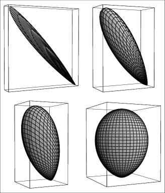
Figure 5: Angular correlation profile (in arbitrary units) of the conditional probability distribution $P(\Omega|\Omega_{0})$ that, in a given tunneling event, an electrons goes into $\Omega$ if the other electron has gone into $\Omega_{0}$. Here we plot $P(\Omega|\Omega_{0})$ as a function of $\Omega$ for fixed $\Omega_{0}\equiv(\theta_{0},\phi_{0})=(\pi/4,0)$. From top-left to bottom-right the radii are: $R=3,1,0.5,0.01\lambda_{F}$. Observe that, as $R$ increases, the angular dependence of the second electron tends to be the conjugate of the first one, i.e. the distribution becomes peaked around $\Omega=(\pi/4,\pi)$. Note also that, for small $R$, $P(\Omega|\Omega_{0})$ becomes $\propto\cos^{2}\theta$ regardless of $\Omega_{0}$.

We have computed the conditional probability distribution $P(\Omega|\Omega_{0})$ for an electron to be emitted into $\Omega\equiv(\theta,\phi)$ given that the other electron is emitted in a fixed direction $\Omega_{0}$. Such a distribution is shown in Fig. 5 for $\Omega_{0}=(\pi/4,0)$. We observe that, for large $R/\lambda_{F}$, the angular distribution of the second electron is quite focussed around $\Omega=(\pi/4,\pi)$, which is mirror-symmetric to $\Omega_{0}$. As $R/\lambda_{F}$ decreases, the angular correlation between electrons disappears and, as a function of $\Omega$, $P(\Omega|\Omega_{0})$ becomes independent of the given value of $\Omega_{0}$. In particular it tends to $\sim\cos^{2}\theta$.

We may also study the probability distribution that one electron is emitted into direction $\Omega$ regardless of the direction chosen by the other electron. This amounts to the calculation of an effective $g(\theta)$ for a finite radius interface to be introduced in an equation like Eq. (38) to compute the current (by symmetry, such a distribution is independent of $\phi$). As expected, one finds such effective angular distribution to be $\sim\cos^{5}\theta$ for large $R$ [see Eq. (44)], which contrasts with the sharp $\Omega$-dependence of the conditional angular distribution $P(\Omega|\Omega_{0})$ for given $\Omega_{0}$.

For small $R$, the effective $g(\theta)$ goes like $\cos^{2}\theta$, i.e. it becomes identical to $P(\Omega|\Omega_{0})$. This coincidence reflects the loss of angular correlations. The $\cos^{2}\theta$ behavior may be understood physically as stemming from a random choice of final ${\bf k}_{\parallel}$, which yields a $\cos\theta$ factor (since $|{\bf k}_{\parallel}|=k_{F}\sin\theta$), weighted by a $\cos\theta$ reduction accounting for the projection of the current over the $z$ direction. An equivalent study for a NN interface yields also $g(\theta)\propto\cos^{2}\theta$. Thus we see that the loss of angular correlations after transmission through a tiny hole makes the NN and NS interfaces display similar angular distributions.

The crossover from $g(\theta)\propto\cos^{2}\theta$ to $\cos^{5}\theta$ as $R$ increases involves a decrease of the width $\Delta\theta$ of the angular distribution. A detailed numerical analysis confirms this result but reveals that $\Delta\theta$ is not a monotonically decreasing function of $R$ (not shown).

VIII Nonlocal entanglement in a two-point interface

Let us turn our attention to a tunneling interface consisting of two small holes, as depicted in Fig. 2(b). By “small” we mean satisfying $R/\lambda_{F}\ll 1$. This is the limit in which the detailed structure of a given hole is not important and the joint behavior of the two holes is a sole function of their relative distance $r$ and the current that would flow through one of the holes if it were isolated. We expect the conclusions obtained in this section to be applicable to similar interfaces made of pairs of different point-like apertures such as, e.g. two point-contacts or two quantum dots weakly coupled to both electrodes recher01 .

The current through a two-point interface has three contributions. One of them is the sum of the currents that would flow through each hole in the absence of the other one. Since the two orifices are assumed to be identical we refer to it as $2I_{0}$, where $I_{0}$ is given in Eq. (56). This contribution collects the events in which the two electrons tunnel through the same opening. A second contribution $I_{e}(r)$ comes from those events in which each electron leaves through a different hole. This is the most interesting contribution since it involves two non-locally entangled electrons forming a spin singlet. The third contribution, $I_{i}(r)$, accounts for the interference between the previous processes.

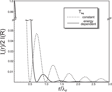
Figure 6: Current density through a two-point interface stemming from non-locally entangled electron pairs, as a function of the distance between points. The dashed line corresponds to the current obtained using an energy-independent hopping approximation whereas in the solid line the correct momentum dependence has been taken into account.

If we write

$$I=2I_{0}+I_{e}(r)+I_{i}(r)\,,$$ (59)

we obtain for the entangled current in the high barrier limit

$$I_{e}(r)=18I_{0}[B^{2}(k_{F}r)+F^{2}(k_{F}r)B^{2}(k_{F}r)]\,,$$ (60)

where $B(x)$ in Eq. (97) and

$$F(x)=3\,\frac{\sin x-x\cos x}{x^{3}}\,.$$ (61)

For $\delta\ll 1$, and noting that we are not interested in tiny distances $r\lesssim\delta\lambda_{F}$, we can write

$$I_{e}(r)=2I_{0}[F^{2}(k_{F}r)+F^{4}(k_{F}r)]e^{-2r/\pi\xi_{0}}\,.$$ (62)

This is a fast decay because of the geometrical prefactor, which goes like $r^{-4}$ for $k_{F}r\gg 1$. For instance, $I_{e}(\xi_{0})/I_{e}(0)\sim 10^{-15}$, with data taken from Al ($\xi_{0}\simeq 10^{3}\lambda_{F}$). For possible comparison with other tunneling models it is interesting to write the entangled conductance $G_{e}(r)\equiv I_{e}(r)/V$ in terms of the normal conductance through one narrow hole, $G_{\rm NN}$. Using Eq. (58), we obtain

$$G_{e}(r)=\frac{h}{2e^{2}}G_{\rm NN}^{2}\,[F^{2}(k_{F}r)+F^{4}(k_{F}r)]e^{-2r/\pi\xi_{0}}\,.$$ (63)

To keep track of the interference terms, it is convenient to adopt a schematic notation whereby $H_{T}=t_{a}+t_{b}$ is the tunneling Hamiltonian through points $a$ and $b$. Then one notes that, as obtained from Eqs. (31), (32) and (35), the total current can be symbolically written as $I\sim|(t_{a}+t_{b})(t_{a}+t_{b})|^{2}$. In this language $I_{0}\sim|t_{a}t_{a}|^{2}$. The $F^{2}$ term in (62) corresponds to $\sim|t_{a}t_{b}|^{2}+|t_{b}t_{a}|^{2}$, while the $F^{4}$ term stems from the interference $\sim(t_{a}t_{b})(t_{b}t_{a})^{*}+{\rm c.c.}$ Altogether, $I_{e}(r)\sim|t_{a}t_{b}+t_{b}t_{a}|^{2}$.

The interference current may be divided into two contributions,

$$I_{i}=I_{i1}+I_{i2}\ ,$$ (64)

corresponding to the different types of outgoing channel pairs which may interfere. The first contribution stems from the interference between both electrons leaving through point $a$ and both electrons leaving through point $b$, $I_{i1}\sim(t_{a}t_{a})(t_{b}t_{b})^{*}+{\rm c.c.}$ One obtains

$$I_{i1}(r)=2I_{0}F^{2}(k_{F}r)\ .$$ (65)

$I_{i2}(r)$ comes from the interference between the channel in which the two electrons leave through the same hole and that in which they exit through different openings, $I_{i2}(r)\sim(t_{a}t_{a})(t_{a}t_{b})^{*}+{\rm c.c.}$, plus three other equivalent contributions, altogether summing

$$I_{i2}(r)=8I_{0}F^{2}(k_{F}r)e^{-r/\pi\xi_{0}}\ .$$ (66)

In the hypothetical case where orifices $a$ and $b$ are connected to different normal electrodes [e.g. when an opaque barrier divides into two halves the normal metal of Fig. 2(b)], the interference contributions (65) and (66) would be absent. Then one would have $I=2I_{0}+I_{e}(r)$.

IX Failure of the momentum-independent hopping approximation

It has been common in the literature on the tunneling Hamiltonian to assume that the tunneling matrix elements appearing in (10) are independent of the perpendicular momenta $k_{z}q_{z}$ (see, for instance, Ref. mahan00 ). Below we show that, for three-dimensional problems, such an assumption is unjustified and leads to a number of physical inconsistencies comm-cancel .

For simplicity we focus on the high barrier limit. To investigate the consequences of the momentum-independent hopping approximation, we replace Eq. (18) by

$$T_{\mathbf{k}\mathbf{q}}=\frac{\tau}{\Omega N(0)}\delta(\mathbf{k}_{\parallel}-\mathbf{q}_{\parallel})\,k_{F}^{2}\,,$$ (67)

i.e. we change $k_{z}q_{z}$ by $k_{F}^{2}$.

Broad interface. For a large NS junction, we find that the total current in units of $I_{V}$ diverges ($x\equiv\cos\theta$):

$$I_{\rm{NS}}=\tau^{4}I_{V}\int_{0}^{1}\frac{dx}{x}\>\frac{x^{2}+\sqrt{x^{4}+\delta^{2}}}{2(x^{4}+\delta^{2})}\rightarrow\infty\,,$$ (68)

i.e. $I_{\rm{NS}}$ grows faster than $A$ for $A\rightarrow\infty$. Eq. (68) is the analogue of Eqs. (38) and (43).

A different divergence occurs for a broad NN tunnel junction:

$$I_{\rm{NN}}=2\tau^{2}I_{V}\int_{0}^{1}\frac{dx}{x}\rightarrow\infty\,,$$ (69)

which contrasts with the finite integral $I_{\rm NN}\sim\int_{0}^{1}dx\,x^{3}$ obtained from inserting (50) into (49).

Local Hamiltonian. If one attempts to derive the real space tunneling Hamiltonian with the assumption (67), one obtains an expression identical to that in Eq. (25) with $\widetilde{L}(z,z^{\prime})$ replaced by

$$\widetilde{M}(z,z^{\prime})=\frac{k_{F}^{2}}{L_{z}}{\sum_{k_{z},q_{z}}}\varphi_{k_{z}}\!(z)\,\varphi^{*}_{q_{z}}\!(z^{\prime})\,.$$ (70)

As in section IV, we use stationary waves for $\varphi_{k_{z},q_{z}}(z)$. Invoking the identity

$$\sum_{k_{z}>0}\sin(k_{z}z)={\cal P}\frac{1}{z}$$ (71)

we obtain

$$H_{T}=\sum_{\sigma}\frac{\tau k_{F}^{2}}{2\pi^{4}N(0)}\int d\mathbf{r}\int_{-L}^{0}\frac{dz}{z}\int_{0}^{L}\frac{dz^{\prime}}{z^{\prime}}\,\psi^{\dagger}_{N}(\mathbf{r},z;\sigma)\psi_{S}(\mathbf{r},z^{\prime};\sigma)+\textrm{H.c.}\,,$$ (72)

where the reference to the principal value has been removed because, in the tunneling limit, the fields vanish linearly at the origin.

If we had chosen plane wave functions for $\varphi_{k_{z},q_{z}}$ in Eq. (70), we would have obtained a different Hamiltonian, namely,

$$H_{T}=\sum_{\sigma}\frac{\tau k_{F}^{2}}{8\pi^{2}N(0)}\int\!d\mathbf{r}\,\psi^{\dagger}_{N}(\mathbf{r},0;\sigma)\psi_{S}(\mathbf{r},0;\sigma)+\textrm{H.c.}\,,$$ (73)

which is some times proposed in the literature (see e.g. Ref. falci01 ). This situation, whereby plane-wave and stationary-wave representations lead to different, both unphysical, local Hamiltonians contrasts with the scenario obtained with the right matrix element. As noted in section IV, the more physical choice (18) leads in both representations (plane and stationary waves) to the correct local Hamiltonian (29). The fact that Eq. (67) leads to a wrong real space Hamiltonian which, moreover, depends on the choice of representation, may be viewed as further proof of the inadequacy of the energy-independent hopping model.

Thermodynamic limit. For a NS interface with $\delta\rightarrow 0$, a dimensional analysis for $A\rightarrow\infty$ suggests that the total current $I_{\rm NS}$ diverges non-thermodynamically like $\sim A^{2}$. For a NN interface, we find the divergence $A\ln A$.

Unitarity. The divergences expressed in Eqs. (68) and (69), as well as the related anomalous thermodynamic behavior, could have been anticipated by noting that, if $T_{\bf kq}$ is assumed to be independent of energy, then Eq. (21) must be multiplied by $(E_{F}/E_{z})^{2}$. As a result, the transmission probability at energy $E_{z}$, which should stay smaller than unity, grows instead as $T(E_{z})\sim E_{z}^{-1}$ for $E_{z}\rightarrow 0$. Such a violation of unitarity necessarily generates a divergent current in the broad interface limit for both NN and NS interfaces.

Nonlocally entangled current. Finally, we note that, using (67), the nonlocally entangled current through two distant points is

$$\tilde{I}_{e}(r)=2\,\tilde{I}_{0}[\tilde{F}^{2}(k_{F}r)+\tilde{F}^{4}(k_{F}r)]e^{-2r/\pi\xi_{0}}\,,$$ (74)

where

$$\tilde{F}(x)=\frac{\sin x}{x}\,,$$ (75)

with the tildes generally referring to the momentum-independent approximation. Here, $\tilde{I}_{0}=81I_{0}$ is the current through one narrow hole. Correspondingly, the entangled conductance $G_{e}(r)$ is written like in Eq. (63) with $F(k_{F}r)$ replaced by $\tilde{F}(k_{F}r)$.

Comparison of Eqs. (62) and (74) indicates that the $r$-dependence of the geometrical prefactor is markedly different: For growing $r$, the nonlocally entangled current decays much more slowly ($r^{-2}$) than its momentum-dependent counterpart ($r^{-4}$). It is interesting to compare the ratios $\lambda(r)\equiv I_{e}(r)/I_{e}(0)$ and $\tilde{\lambda}(r)\equiv\tilde{I}_{e}(r)/\tilde{I}_{e}(0)$. While $\lambda(0)=\tilde{\lambda}(0)=1$ by construction, the ratio $\lambda/\tilde{\lambda}$ becomes $\sim 6\times 10^{-4}$ and $2\times 10^{-7}$ for $r/\lambda_{F}=20$ and $10^{3}$, respectively.

Interference terms. As expected from the comparison of Eqs. (62) and (74), the interference contributions are identical to those discussed in the previous section with $F(k_{F}r)$ replaced by $\tilde{F}(k_{F}r)$ in Eqs. (65) and (66).

Generality of the model. An important question is whether our results for the entangled and interference current through pairs of tiny geometrical holes apply to other, more realistic pairs of small interfaces such as two point contacts or two quantum dots recher01 . The fact that the decay with distance of the entangled current reported in Refs. deutscher00 ; recher01 ; falci01 ; apinyan02 ; melin02 ; feinberg02 ; recher02 ; feinberg03 ; recher03 follows the same law as Eqs. (74) and (75) (except for the $\tilde{F}^{4}$ term there neglected), suggests that such is indeed the case. Below we prove this expectation.

Due to Eq. (30), the sum in Eq. (V) involves

$$\sum_{\mathbf{q}}\frac{u_{\mathbf{q}}v_{\mathbf{q}}}{E_{\mathbf{q}}}q_{z}^{2}e^{-i{\bf q}_{\parallel}\cdot({\bf r}_{1}-{\bf r}_{2})}\,.$$ (76)

This sum over q is clearly affected by the presence of the $q_{z}^{2}$ factor, yielding a result $\propto F(k_{F}r)$, with $r=|{\bf r}_{1}-{\bf r}_{2}|$. In the momentum-independent hopping approximation, $q_{z}^{2}$ is replaced by $k_{F}^{2}$, rendering the sum $\propto\tilde{F}(k_{F}r)$. In fact, the two functions are related:

$$\left.\frac{\partial^{2}}{\partial z^{2}}\tilde{F}(k_{F}\sqrt{r^{2}+z^{2}})\right|_{z=0}=\frac{1}{3}k_{F}^{2}F(k_{F}r)\ .$$ (77)

We note that the distance dependence is determined by the properties of the superconductor and not by those of the normal electrode. If a quantum dot mediates between the superconductor and the normal metal, then an effective hopping must be introduced in (76) which, however, does not add any new momentum dependence [see Eq. (11) of Ref. recher01 ]. Departure from the specific type of contact here considered will translate only into a different value of $I_{0}$, the distance dependent prefactor remaining identical. We notice, however, that the preceding discussion is restricted to the case where quasiparticle propagation is ballistic in both electrodes, i.e. we neglect the effect of impurities or additional barriers hekk94 .

X Summary

We have investigated the electron current through a NS tunneling structure in the regime $k_{B}T\ll eV\ll\Delta$ where Andreev reflection is the dominant transmissive channel. We have rigorously established the physical equivalence between Cooper pair emission and Andreev reflection of an incident hole. A local tunneling Hamiltonian has been derived by properly truncating that of an infinite interface in order to describe tunneling through an arbitrarily shaped interface. Such a scheme has been applied to study transport through a circular interface of arbitrary radius and through an interface made of two tiny holes. In the former case, the angular correlations between the two emitted electrons have been elucidated and shown to be lost as the interface radius becomes small. We have also investigated how the thermodynamic limit is recovered, showing that, due to the destructive interference between possible exit points, it is achieved for radii a few times the Fermi wave length. For the case of a two-point interface, we have calculated the nonlocally entangled current stemming from processes in which each electron leaves the superconductor through a different orifice. We have found that, as a function of the distance between openings, such an entangled current decays quickly on the scale of one Fermi wave length. The interference between the various outgoing two-electron channels has also been investigated and shown to yield contributions comparable to the nonlocally entangled current. We have found that, in a three-dimensional problem, it is important to employ hopping matrix elements with the right momentum dependence in order to obtain sound physical results in questions having to do with the local tunneling Hamiltonian (whose correct form has also been obtained from a tight-binding description), the thermodynamic limit, the preservation of unitarity, and the distance dependence of the nonlocally entangled current through a two-point interface. An important virtue of the method here developed is that it enables the systematic study of Cooper pair emission through arbitrary NS tunneling interfaces and opens the door to a convenient exploration of the fate of Cooper pairs in the normal metal and, in particular, to the loss of phase and spin coherence between emitted electrons.

Appendix A Discrete vs. continuum space

Take a discrete chain made of $N$ sites with period $a$ described by the Hamiltonian

$$H_{0}=-t\sum_{i=1}^{N-1}c_{i+1}^{\dagger}c_{i}+\rm{H.c.}\,,$$ (78)

where $t=\hbar^{2}/2ma^{2}>0$ is the hopping parameter that yields an effective mass $m$ in the continuum limit.

The eigenstates of this chain are of the form

$$|\phi_{n}\rangle=\left(\frac{2}{N+1}\right)^{1/2}\sum_{i=1}^{N}\sin(k_{n}z_{i})c^{\dagger}_{i}|{\rm vac}\rangle\,,$$ (79)

where $z_{i}=ia$ and $k_{n}=\pi n/a(N+1)$ with $i,n\in[1,N]$. The eigenvalues are

$$E_{n}=-2t\cos(k_{n}a)\,.$$ (80)

The basis set $\{|\phi_{n}\rangle\}$ is orthonormal. Thus we may write

$$c^{\dagger}_{k_{n}} = \left(\frac{2}{N+1}\right)^{1/2}\sum_{i=1}^{N}\sin(k_{n}z_{i})c^{\dagger}_{i}\,,$$ (81)

$$c^{\dagger}_{i} = \left(\frac{2}{N+1}\right)^{1/2}\sum_{n=1}^{N}\sin(k_{n}z_{i})c^{\dagger}_{k_{n}}\,.$$ (82)

We write the transfer Hamiltonian between two $N$-site chains as

$$H_{T} = -t^{\prime}a^{\dagger}_{1}b_{-1}+\rm{H.c}$$ (83)

$$= \frac{2t^{\prime}}{N+1}\sum_{n=1}^{N}\sum_{m=1}^{N}\sin(k_{n}a)\sin(k_{m}a)a^{\dagger}_{k_{n}}b_{k_{m}}+\rm{H.c.}~{}~{}~{}~{}~{}~{}$$ (84)

which may be treated as a small perturbation when $t^{\prime}\ll t$.

To investigate the continuum limit, we take $a\rightarrow 0$ and $t\rightarrow\infty$ so that $m$ and $k_{F}$ remain finite. We also take $N\gg 1$. Noting that the sine functions in (84) can be approximated by their arguments $k_{n}a\lesssim k_{F}a\ll 1$ and that $k_{\rm{max}}=\pi/a\rightarrow\infty$, we get

$$H_{T}=\frac{2t^{\prime}a^{3}}{L}\sum_{k,q>0}k\>q\,a^{\dagger}_{k}b_{q}+\rm{H.c.}$$ (85)

This Hamiltonian is bilinear in the momenta of the electron on the right and left chain. If we were in 3D we would specify that the bilinearity refers to the momenta perpendicular to the interface plane. This hamiltonian is analogous to that which we proposed for the continuum Bardeen theory in the case of a high barrier [see Eqs. (10) and (18)].

We may work out the corresponding Hamiltonian in real space. For that we note that, in the continuum limit, $H_{T}$ in Eq. (83) can be expressed in terms of field operators evaluated in $z=\pm a$. When $a\rightarrow 0$, the field operators can be expanded as

$$\psi(a)=\psi(0)+a\left.\frac{d\psi(z)}{dz}\right|_{z=0}+{\cal O}(a^{2})\,,$$ (86)

where $\psi(0)=0$ is a condition that results naturally from the properties of the wave functions in a chain starting in $i=1$ or $i=-1$. For such chains, $i=0$ is an imaginary point where the wave function necessarily vanishes; it is the place where we would locate the hard wall in a continuum description sols89 . Then the tunneling Hamiltonian can be written

$$H_{T}=t^{\prime}a^{3}\left.\frac{d\psi^{\dagger}_{R}(z)}{dz}\right|_{z=0}\left.\frac{d\psi_{L}(z^{\prime})}{dz^{\prime}}\right|_{z^{\prime}=0}+\textrm{H.c.}$$ (87)

This Hamiltonian is exactly the one-dimensional version of that in Eq. (29). The fact that we have derived it from a completely different set of physical arguments should be viewed as a definite proof of the adequacy of the tunneling Hamiltonians proposed in section IV. The Hamiltonians (85) and (87) have been obtained in the continuum limit. On the other hand, Eqs. (18) and (29) were derived for high barriers or, equivalently, low energies. Clearly, this is not a coincidence, since it is at low energies where the long wavelengths make the electron move in the chain as in continuum space.

Appendix B Total current vs. interface radius

To calculate the total current as a function of the interface radius $R$ we have to evaluate the matrix element (V) using hopping energies obtained from the tunneling Hamitonian (30). In the resulting expression we need to integrate over the final momenta of the two electrons in the normal metal, the momentum of the intermediate virtual state consisting of a quasiparticle in the superconductor, as well as the coordinates of the points where each electron crosses the interface area. The integrations over the momenta in the final state lead to four angular integrals ($\theta_{1,2}\in[0,\pi/2];\varphi_{1,2}\in[0,2\pi]$), the moduli being fixed by the condition $k_{B}T,eV\rightarrow 0$. The integration over the superconductor excited states leads to three integrals: $\theta_{s}\in[0,\pi],\varphi_{s}\in[0,2\pi],q\in[0,q_{c}]$. On the other hand, integration over the hopping points of each electron leads to two interface integrals ($r_{1,2}\in[0,R]$, $\theta_{r1,r2}\in[0,2\pi]$), which makes four more integrals, totalling eleven real variables to be integrated. Using the symmetry property that the integrand is independent of one azimuthal angle, and solving analytically the four real space integrals, we are left with six non-reducible nested integrals of strongly oscillating functions.

We define $\vec{\kappa}\equiv\mathbf{k}/k_{F}$, $\vec{\varrho}\equiv\mathbf{q}/k_{F}$. Since the modula of the final momenta are fixed by conservation requirements, we may write $\kappa_{\parallel i}=\sin\theta_{i}$, $\kappa_{zi}=\cos\theta_{i}$ ($i=1,2$). For the virtual states in the superconductor: $\varrho_{\parallel}=\varrho\sin\theta_{s}$, $\varrho_{z}=\varrho\cos\theta_{s}$.

The general, exact formula for the total current as a function or $R$ is

$$I(R) = I_{V}\tau^{4}\frac{(k_{F}R)^{2}}{4\pi^{3}}\int d\Omega_{1}\int d\kappa_{2z}\kappa_{1z}^{2}\kappa_{2z}^{2}e^{2p_{0}w[1-b(\kappa_{1z},\kappa_{2z})]}$$

$$\times \left[\frac{2}{\pi}\int d\varrho\frac{\delta}{(\varrho^{2}-1)^{2}+\delta^{2}}\varrho^{4}\int d\Omega_{s}e^{p_{0}w[1-b(\varrho_{z})]}\prod_{j=1,2}a(\kappa_{zj},\varrho_{z})J(|\vec{\varrho}_{\parallel}-\vec{\kappa}_{1\parallel}|,|\vec{\varrho}_{\parallel}+\vec{\kappa}_{2\parallel}|)\right]^{2},$$

where $J$ is a short-hand notation for

$$J(x,y)\equiv\frac{J_{1}(k_{F}R\,x)J_{1}(k_{F}R\,y)}{x\,y}\,.$$ (89)

The first-order Bessel functions result from the exact integration over the tunneling points ${\bf r}_{1}$ and ${\bf r}_{2}$.

For $\delta\rightarrow 0$, the Lorentzian becomes a delta function and the integral over $\varrho$ is evaluated exactly. We get (with $u$ still arbitrary)

$$I(R) = I_{V}\tau^{4}\frac{(k_{F}R)^{2}}{4\pi^{3}}\int d\Omega_{1}\int d\kappa_{2z}\kappa_{1z}^{2}\kappa_{2z}^{2}e^{2p_{0}w[1-a(\kappa_{1z},\kappa_{2z})]}$$ (90)

$$\times \left[\int d\Omega_{s}e^{p_{0}w[1-b(\varrho_{z})]}\prod_{j=1,2}a(\kappa_{zj},\varrho_{z})J(|\vec{\varrho}_{\parallel}-\vec{\kappa}_{1\parallel}|,|\vec{\varrho}_{\parallel}+\vec{\kappa}_{2\parallel}|)\right]^{2}.$$

For $\delta$ arbitrary and $u\gg 1$, Eq. (B) becomes

$$I(R)=I_{V}\tau^{4}\frac{(k_{F}R)^{2}}{4\pi^{3}}\int d\Omega_{1}\int d\kappa_{2z}\kappa_{1z}^{2}\kappa_{2z}^{2}\left[\frac{2}{\pi}\int d\varrho\frac{\delta}{(\varrho^{2}-1)^{2}+\delta^{2}}\varrho^{4}\int d\Omega_{s}J(|\vec{\varrho}_{\parallel}-\vec{\kappa}_{1\parallel}|,|\vec{\varrho}_{\parallel}+\vec{\kappa}_{2\parallel}|)\right]^{2}.$$ (91)

Finally, for both $\delta\rightarrow 0$ and $u\gg 1$, we obtain

$$I(R)=I_{V}\tau^{4}\frac{(k_{F}R)^{2}}{4\pi^{3}}\int d\Omega_{1}\int d\kappa_{2z}\kappa_{1z}^{2}\kappa_{2z}^{2}\left[\int d\Omega_{s}J(|\vec{\varrho}_{\parallel}-\vec{\kappa}_{1\parallel}|,|\vec{\varrho}_{\parallel}+\vec{\kappa}_{2\parallel}|)\right]^{2},$$ (92)

which for $k_{F}R\ll 1$ leads to Eq. (56) in the main text. This is easy to see considering that $\lim_{x\rightarrow 0}J_{1}(k_{F}R\,x)/x=k_{F}R/2$.

Even after making $\delta,u^{-1}\rightarrow 0$, the resulting expression (92) is such that a numerical integration for arbitrary $R$ is not yet possible. In order to evaluate (90) and (92) numerically we need to introduce a set of two approximations which are good for $k_{F}R\gg 1$ and reasonable for intermediate $R$. To introduce the first approximation we go back to the original expression (31), where the space coordinates have not yet been integrated. Then we shift from the two space coordinates $(\mathbf{r}_{1},\mathbf{r}_{2})$ to center-of-mass and relative coordinates $(\mathbf{r}_{c},\mathbf{r})$. The integration domain of the center-of-mass coordinate $\mathbf{r}_{c}$ is still a circle of radius $R$. However, the integration region of the relative coordinate $\mathbf{r}$ is more complicated: It is eye-shaped and centered around $\mathbf{r}_{c}$. The first approximation consists in assuming that, for all $\mathbf{r}_{c}$, the integration domain of the relative coordinate is circular instead of eye-shaped. The area of such a circular region is a free parameter which can be adjusted by, e.g. comparing the approximate result with the exact calculation for those values of $R$ for which the latter can be performed.

It is intuitive (and rigorously proved in subsection VII.B) that, because of diffraction, when $R\lesssim\lambda_{F}$, the parallel momentum is not conserved and, in particular, the two electrons do not leave necessarily with opposite parallel momenta [see Fig. (5)]. Nevertheless, as $R$ increases the interface begins to be large enough so as to permit parallel momentum to become better conserved. A quasi-delta function $\widetilde{\delta}(\mathbf{k}_{1\parallel}+\mathbf{k}_{2\parallel})$ effectively appears. In particular we have: $\lim_{R\rightarrow\infty}J_{1}(k_{\parallel}R)/k_{\parallel}=2\pi\delta(\mathbf{k}_{\parallel})/R$. Thus, our second approximation consists in assuming that, for all $R>\lambda_{F}$, the quasi-delta is an exact delta: $\widetilde{\delta}\rightarrow\delta$. This is equivalent to the assumption that there is no diffraction, i.e. that we work in the ray optics limit. This approximation becomes exact as $R\rightarrow\infty$ and it is a reasonable one for finite radii. Of course, this approximation fails for $R\lesssim\lambda_{F}$, yielding a wrong $R^{4}$ behavior.

With the two previous approximations we can reduce the number of numerical integrals from five to three. To write the resulting expressions, let us introduce some compact notation. We define $x\equiv\cos\theta$ (where $\theta$ is the angle formed by the outgoing momentum with the direction normal to the interface), $y\equiv\cos\theta_{q}$ ($\theta_{q}$ having a similar definition within the superconductor), $\lambda\equiv k_{F}|\mathbf{r}_{c}|$, and $\mu\equiv k_{F}|\mathbf{r}|$.

For $\delta\rightarrow 0$ and arbitrary $u$ we obtain

$$I(R)\simeq I_{V}\tau^{4}\int_{0}^{1}dx\>x^{3}e^{2p_{0}w[1-b(x)]}\left\{\int_{0}^{k_{F}R}d\lambda\>\frac{2\lambda}{(k_{F}R)^{2}}\int_{0}^{1}dy\frac{r(\lambda)y^{2}}{x^{2}-y^{2}}[a(x,y)]^{2}e^{2p_{0}w[1-b(y)]}\right.$$

$$\left.\times\left[\sqrt{1-y^{2}}\;J_{0}\!\!\left(r(\lambda)\sqrt{1-x^{2}}\right)J_{1}\!\!\left(r(\lambda)\sqrt{1-y^{2}}\right)-\sqrt{1-x^{2}}\;J_{0}\!\!\left(r(\lambda)\sqrt{1-y^{2}}\right)J_{1}\!\!\left(r(\lambda)\sqrt{1-x^{2}}\right)\right]\right\}^{2}\,,$$

where $r(\lambda)$ is the radius of the approximate circular domain over which the relative coordinate ${\bf r}$ is integrated. If the circle is assumed to have the same area as the eye, we obtain

$$r(\lambda)\equiv\sqrt{\frac{8}{\pi}}\left[(k_{F}R)^{2}\arccos\left(\frac{\lambda}{k_{F}R}\right)-\lambda\sqrt{(k_{F}R)^{2}-\lambda^{2}}\right]^{1/2},$$ (94)

but in practice this criterion is found to overestimate the total current. Thus we decide to adopt the ansatz

$$r(\lambda)\equiv 2k_{F}R\left(1-\frac{\lambda}{k_{F}R}\right)^{\alpha}\,,$$ (95)

where $\alpha$ is a parameter to be adjusted by comparison with the exact solution in those cases where it can be computed. In particular, $\alpha$ has been adjusted from the last two exact numerical values of each curve, i.e. from the two largest computationally possible radii. We note that both (94) and (95) satisfy the requirement $r(\lambda)\rightarrow 2k_{F}R$ for $\lambda\rightarrow 0$. The value $\alpha=1$ corresponds to the case where the circle is chosen to be the maximum circle which fits within the eye-shaped integration domain. As expected, this criterion underestimates the current. The formula (94), which overestimates the result, can be approximated with $\alpha\approx 0.7$. Thus it comes as no surprise that the value of $\alpha$ obtained by comparing with the exact result (when available) is an intermediate number, namely, $\alpha=0.84$, which has been used for the NS curves in Fig. 4.

For arbitrary $\delta$ and $u\gg 1$, the total current becomes

$$I(R) \simeq I_{V}\tau^{4}\int_{0}^{1}dx\>x^{3}\left[\frac{2}{(k_{F}R)^{2}}\int_{0}^{k_{F}R}d\lambda\>\lambda\int_{0}^{r(\lambda)}d\mu\>\mu J_{0}(\mu\sqrt{1-x^{2}})B(\mu)\right]^{2}\,,$$ (96)

$$B(\mu) = \left\{\frac{\sin[S(\delta)\mu)]}{\mu^{3}}-\frac{\sqrt[4]{1+\delta^{2}}\cos[\arctan\delta/2+S(\delta)\mu]}{\mu^{2}}\right\}e^{-D(\delta)\mu}\,,$$ (97)

where

$$S(\delta)=\left(\frac{\sqrt{1+\delta^{2}}+1}{2}\right)^{1/2}\stackrel{{\scriptstyle\delta\ll 1}}{{\rightarrow}}1\,,$$ (98)

$$D(\delta)=\left(\frac{\sqrt{1+\delta^{2}}-1}{2}\right)^{1/2}\stackrel{{\scriptstyle\delta\ll 1}}{{\simeq}}\frac{\delta}{2}\,.$$ (99)

Thus, for $\delta\ll 1$ we may write

$$B(\mu)\simeq\left[\frac{\sin(\mu)}{\mu^{3}}-\frac{\cos(\mu+\delta/2)}{\mu^{2}}\right]e^{-\delta\mu/2}\,.$$ (100)

The effect of the phase-shift $\delta/2$ is only appreciable for $\mu\lesssim\delta$, i.e. for $r\lesssim\delta\lambda_{F}\ll\lambda_{F}$, as can be seen by expanding $B(\mu)$ for small $\mu$:

$$B(\mu)=\frac{\delta}{2\mu}+\frac{1}{3}-\frac{\delta\mu}{4}-\frac{\delta^{2}}{8}+{\cal O}(\delta^{4},\mu^{2}).$$ (101)

The phase-shift generates a divergence for $\mu\rightarrow 0$. Although integrable thanks to the multiplying $\mu$ factor in Eq. (96), this divergence affects the final result. Its range of relevance may be estimated by making $\delta/2\mu$ equal to the limiting value $1/3$ which one would obtain with $\delta=0$. This yields a range $r_{0}=(3/4\pi)\delta\lambda_{F}$, which will be washed out by any realistic momentum cutoff $q_{c}\sim k_{F}\ll k_{F}/\delta$.

Finally, we note that comparison of Eqs. (62) and (100) clearly reveals that the entangled current $I_{e}(r)$ given in (62) is essentially proportional to $B^{2}(k_{F}r)$. As discussed in Sec. IX, $I_{e}(r)$ decays faster than the prefactor obtained from momentum-independent hopping matrix elements [see Eq. (74)]. The current increase which results from such an unphysical approximation translates into a divergent thermodynamic limit (see also Sec. IX).

References

- (1) A. F. Andreev, Zh. Ekps. Teor. Fiz. 46, 1823 (1964) [Sov. Phys. JETP 19, 1228 (1964)]; 49, 655 (1966) [22, 455 (1966)].
- (2) J. Demers and A. Griffin, Can. J. Phys. 49, 285 (1970).
- (3) G. E. Blonder, M. Tinkham and T. M. Klapwijk, Phys. Rev. B 25, 4515 (1982).
- (4) M. Tinkham, Introduction to Superconductivity, 2nd ed. (McGraw-Hill, New York, 1996).
- (5) J. M. Byers and M. E Flatté, Phys. Rev. Lett. 74, 306 (1995).
- (6) J. Torres and T. Martin, Eur. Phys. J. B 12, 319 (1999).
- (7) G. Deutscher and D. Feinberg, Appl. Phys. Lett. 76, 487 (2000).
- (8) P. Recher, E. V. Sukhorukov and D. Loss, Phys. Rev. B 63, 165314 (2001).
- (9) G. Falci, D. Feinberg and F. W. J. Hekking, Europhys. Lett. 54, 255 (2001).
- (10) R. Mélin, J. Phys.: Condens. Matter 13, 6445 (2001).
- (11) G. B. Lesovik, T. Martin and G. Blatter, Eur. Phys. J. B 24, 287 (2001).
- (12) V. Apinyan and R. Mélin, Eur. Phys. J. B 25, 373 (2002).
- (13) R. Mélin and D. Feinberg, Eur. Phys. J. B 26, 101 (2002).
- (14) D. Feinberg and G. Deutscher, Physica E 15, 88 (2002).
- (15) P. Recher and D. Loss, Phys. Rev. B 65, 165327 (2002).
- (16) N. M. Chtchelkatchev, G. Blatter, G. B. Lesovik and T. Martin, Phys. Rev. B 66 161320 (2002).
- (17) D. Feinberg, Eur. Phys. J. B 36, 419 (2003).
- (18) P. Recher and D. Loss, Phys. Rev. Lett. 91, 267003 (2003).
- (19) P. Samuelsson, E. V. Sukhorukov, and M. Büttiker, Phys. Rev. Lett. 91, 157002 (2003).
- (20) M. Kupka, Phys. C 221, 346 (1994).
- (21) M. Kupka, Phys. C 281, 91 (1997).
- (22) P. G. de Gennes, Superconductivity of Metals and Alloys, (Addison-Wesley, Reading, 1989).
- (23) C. W. J. Beenakker, in Mesoscopic Quantum Physics, E. Akkermans, G. Montamboux, and J. L. Pichard, eds. (North-Holland, Amsterdam, 1995).
- (24) J. Sánchez-Cañizares and F. Sols, J. Phys.: Condens. Matter 7, L317 (1995).
- (25) J. Sánchez-Cañizares and F. Sols, Phys. Rev. B 55, 531 (1997).
- (26) R. Kümmel, Z. Physik 218, 472 (1969).
- (27) F. Sols and J. Sánchez-Cañizares, Superlatt. and Microstruct. 25, 627 (1999).
- (28) C. J. Lambert, J. Phys.: Condens. Matter 3, 6579 (1991).
- (29) C. W. J. Beenakker, Phys. Rev. B 46, 12841 (1992).
- (30) H. Nakano and H. Takayanagi, Phys. Rev. B 50, 3139 (1994).
- (31) A. Levy Yeyati, A. Martín-Rodero, F. J. García-Vidal, Phys. Rev. B 51, 3743 (1995).
- (32) J. Sánchez-Cañizares and F. Sols, J. Low Temp. Phys. 122, 11 (2001).
- (33) J. R. Kirtley, Phys. Rev. B 47, 11379 (1992).
- (34) J. Bardeen, Phys. Rev. Lett. 6, 57 (1961).
- (35) G. D. Mahan, Many-Particle Physics, 3rd ed. (Kluwer Academic/Plenum, New York, 2000), p. 561.
- (36) R. E. Prange, Phys. Rev. 131, 1083 (1963).
- (37) A. Galindo and P. Pascual, Quantum Mechanics (Springer, Berlin, 1990).
- (38) P. V. Gray, Phys. Rev. 140, 179 (1965).
- (39) The low-energy linear dependence and the related bilinear dependence is implicit in Ref. duke69 . We note, however, that here we find perfect agreement between Bardeen’s perturbative method and the exact results in the tunneling limit.
- (40) C. B. Duke, Tunneling in Solids, (Academic Press, New York and London, 1969), p. 218.
- (41) C. J. Chen, Phys. Rev. B 42, 8841 (1990).
- (42) E. Merzbacher, Quantum Mechanics, 3rd ed. (John Wiley & Sons, New York, 1998), ch. 20.
- (43) Note that, as defined in Eq. (34), the final state is identical to the state . Thus, when summing over final states, one must avoid double counting. Specifically, in Eq. (31), is to be understood as , where is an unrestricted sum over indices .
- (44) A study of the angular dependence of Andreev reflection in the broad interface limit has been presented in Ref. mortensen99 . However, it is restricted to a delta barrier interface and consider the case where is a doped semiconductor.
- (45) N. A. Mortensen, K. Flensberg and A. P. Jauho, Phys. Rev. B 59, 10176 (1999).
- (46) There, under the constraint of a given total current, entropy is maximized by the electron system adopting a displaced Fermi sphere configuration which exactly yields the law.
- (47) R. Landauer, IBM J. Res. Dev. 1, 223 (1957); M. Büttiker, Phys. Rev. Lett. 57, 1761 (1986); A. Szafer and A. D. Stone, IBM J. Res. Dev. 32, 384 (1988).
- (48) For a broad interface, is conserved and can be identified with . However, invoking trace invariance confers general validity to the argument and makes it more rigorous in the particular case of a broad interface embedded in an even broader wire.
- (49) Together with the factor appearing in the definition (39), this factor yields the geometrical correction given by Ref. sharvin65 and cited in Ref. blonder82 . We emphasize however that such correction applies only to the normal conductance, as derived in Ref. sharvin65 , but not to the NS interface where, rather, the correct geometrical correction is , as implicitly noted in Eqs. (39) and (47).
- (50) Yu. V. Sharvin, Zh. EKsp. Teor. Fiz. 48, 984 (1965) [Sov. Phys.–JETP 21, 655 (1965)].
- (51) H. A. Bethe, Phys. Rev. 66, 163 (1944).
- (52) We do not rule out, however, that the errors derived from the use of Eq. (67) may cancel in the calculation of some physical quantities such as e.g. the ratio between the critical current and the normal conductance of a superconducting tunnel junction ambegaokar63 ; mahan00 .
- (53) V. Ambegaokar and A. Baratoff, Phys. Rev. Lett. 10, 486 (1963).
- (54) F. W. J. Hekking and Yu. V. Nazarov, Phys. Rev. B 49, 6847 (1994).
- (55) F. Sols, M. Macucci, U. Ravaioli, and K. Hess, J. Appl. Phys. 66, 3892 (1989).