The signal-to-noise analysis of the Little-Hopfield model revisited

Abstract

Using the generating functional analysis an exact recursion relation is derived for the time evolution of the effective local field of the fully connected Little-Hopfield model. It is shown that, by leaving out the feedback correlations arising from earlier times in this effective dynamics, one precisely finds the recursion relations usually employed in the signal-to-noise approach. The consequences of this approximation as well as the physics behind it are discussed. In particular, it is pointed out why it is hard to notice the effects, especially for model parameters corresponding to retrieval. Numerical simulations confirm these findings. The signal-to-noise analysis is then extended to include all correlations, making it a full theory for dynamics at the level of the generating functional analysis. The results are applied to the frequently employed extremely diluted (a)symmetric architectures and to sequence processing networks.

1 Introduction

During the last number of years, the treatment of dynamics using generating functional techniques (GFA) has received a lot of attention in the field of statistical mechanics of disordered systems, in particular neural networks (see, e.g., [1]–[4] and references therein). Such a treatment allows for the exact solution of the dynamics and finds all relevant physical order parameters at any time step via the derivatives of a generating functional [5]–[8]. An alternative method to study dynamics of neural networks is the so called signal-to-noise analysis (SNA) or statistical neurodynamics (see, e.g., [9]–[12]) where the idea is to start from a splitting of the local field into a signal part originating from the pattern to be retrieved and a noise part arising from the other patterns. The differences in the existing versions of this approach consist out of the different treatments of this noise term, ranging from the assumption that it is Gaussian with various approximations for its variance [9, 10, 13] to a supposedly exact treatment [14, 15].

In two recent papers some comparisons have been made between the two methods for a sequence processing network [4] respectively the fully connected Blume-Emery-Griffiths network [2]. For the first system, surprisingly, the order parameter equations obtained through the exact GFA solution are shown to be completely equivalent to those of statistical neurodynamics, known to be an approximation that assumes Gaussian noise. These theoretical results are verified by computer simulations. We recall that this system contains no feedback correlations. For the second system that is fully connected and, hence, does contain feedback correlations, it has been shown that the results of the GFA and SNA coincide up to the third time step. Some numerical experiments then indicated that they may differ for further time steps, certainly for those parameters of the system corresponding to spin-glass behaviour.

The idea of the present work is to perform a systematic analytical study of the relationship between both techniques using the fully connected Little-Hopfield model. In order to do so, we take the GFA one step further by deriving a recursion relation for the effective local field. To our knowledge such a recursion relation has not yet been reported upon in the literature. Furthermore, it is precisely this relation that we use as basis for studying the correspondence between both methods.

For the fully connected model we show that the SNA as it has been applied up to now in fact approximates the exact dynamics because it forgets about a part of the correlations. We discuss the physics behind such a short-memory approximation and explain why it leads to very good results in the case of retrieval. Moreover, we show how to apply the SNA correctly leading to a complete equivalence with the GFA. The results obtained are applied to other architectures and to sequence processing networks.

The paper is organized as follows. In Section 2 we recall the fully connected Little-Hopfield model and discuss the SNA approach to solve its dynamics. Section 3 shortly reviews the GFA and derives recursion relations for the effective local field in this framework. Section 4 introduces the short-memory approximation and shows how this reduces the results of the GFA to those of the SNA. It also explains the physics behind this approximation and discusses some numerical results. Section 5 presents a scheme how to apply exactly the SNA. In section 6 we apply our findings to the extremely diluted symmetric and asymmetric architectures and to sequence processing models. Finally, Section 7 contains some concluding remarks.

2 Signal-to-noise analysis of the Little-Hopfield model

2.1 The Little-Hopfield model

By now, the Little-Hopfield model is a standard model for associative memory and can be found in many textbooks (see, e.g, [11]). Consider a system of $N$ Ising spins $\sigma_{i}$, $i=1,\dots,N$. We want to store $p=\alpha N$ patterns ${\boldsymbol{\xi}}^{\mu}=\{\xi^{\mu}_{1},\dots,\xi^{\mu}_{N}\}$, $\mu=1,\dots,p$, independent and identically distributed with respect to $i$ and $\mu$. The local field in neuron $i$ is defined by

$$h_{i}(t)=\sum_{j=1}^{N}J_{ij}\,\sigma_{j}(t)\,,$$ (1)

with the couplings given by the Hebb rule

$$J_{ij}=\frac{1}{N}\sum_{\mu=1}^{p}\xi_{i}^{\mu}\xi_{j}^{\mu}\,,\quad J_{ii}=0\ .$$ (2)

All neurons are updated in parallel according to the Glauber dynamics

$$\mbox{Prob}[\sigma_{i}(t+1)=s|h_{i}(t)]=\frac{e^{\beta sh_{i}(t)}}{2\cosh(\beta h_{i}(t))}\ ,\quad s=\pm 1\,,$$ (3)

which becomes, in the limit $\beta=1/T\to\infty$, equivalent to the gain function formulation

$$\sigma_{i}(t+1)=\mbox{sgn}(h_{i}(t))\ .$$ (4)

In general, we write

$$\sigma_{i}(t+1)=g(h_{i}(t))\,.$$ (5)

The long time behaviour of the system is governed by the Hamiltonian [16]

$$H=-\frac{1}{\beta}\sum_{i}\ln[\cosh(\beta h_{i}(t))]\,.$$ (6)

The thermodynamic and retrieval properties are visualized in the $(T-\alpha)$ phase diagram [17]. There is a transition curve starting at $T=0,\alpha=0.138$ and ending at $T=1,\alpha=0$ beyond which the system does not retrieve any patterns anymore and behaves like a spin-glass. For higher temperatures the system undergoes a transition to the paramagnetic phase.

The parallel dynamics of this model using both the SNA and GFA and, especially, the comparison between these approaches is the subject of the following sections.

2.2 Signal-to-noise analysis

In order to keep this paper self-contained we shortly review the signal-to-noise analysis. We assume that the system has an initial finite overlap with one of the patterns, say the first one, which we call condensed. The other patterns (non-condensed) act as noise, making it harder for the network to retrieve the condensed pattern.

We first focus on zero temperature. The key idea is to separate the signal from the noise in the local field

$$h_{i}(t)=\xi_{i}^{1}\frac{1}{N}\sum_{j}\xi_{j}^{1}\sigma_{j}(t)+\frac{1}{N}\sum_{\mu\neq 1}\xi^{\mu}_{i}\sum_{j}\xi_{j}^{\mu}\sigma_{j}(t)-\alpha\sigma_{i}(t)$$ (7)

whereby it is technically convenient to include the self-interaction and subtract it again leading to the term $\alpha\sigma_{i}(t)$. Quantities that have a site-index, or an index $N$ are quantities for a finite system. We define the overlap, respectively the residual overlap by

$$m_{N}(t)=\frac{1}{N}\sum_{j}\xi_{j}^{1}\sigma_{j}(t)\,,\qquad r_{N}^{\mu}(t)=\frac{1}{\sqrt{N}}\sum_{j}\xi_{j}^{\mu}\sigma_{j}(t)\,,\quad\mu>1\,.$$ (8)

The local field (7) then becomes

$$h_{i}(t)=\xi_{i}^{1}m_{N}(t)+\frac{1}{\sqrt{N}}\sum_{\mu\neq 1}\xi^{\mu}_{i}r^{\mu}_{N}(t)-\alpha\sigma_{i}(t)\,.$$ (9)

Our aim is to determine the form of the local field in the thermodynamic limit $N\to\infty$. To the signal term we apply the law of large numbers (LLN)

$$\lim_{N\to\infty}m_{N}(t)\stackrel{{\scriptstyle{\mathcal{P}r}}}{{=}}m(t)$$ (10)

where the convergence is in probability. Taking a closer look at the second term in (9), we could apply the central limit theorem (CLT) if all the terms in the sum would be independent. This, of course, depends on the architecture and it is true, e.g., for asymmetrically extremely diluted models [18, 19]. In general, there are non-trivial correlations between the terms and the different implementations of the SNA mentioned before treat these correlations in a different way.

For the fully connected architecture at hand, the most naive and simple approach [13] is to keep the assumption that all terms in the sum are uncorrelated, and that one can simply apply the CLT theorem to the second term in (9). The local field becomes normally distributed with mean $\xi_{i}^{1}m(t)$ and variance $\alpha$. This approach has then been refined in the theory of statistical neurodynamics [9]. There one also assumes that the noise part of the local field is normally distributed but one calculates explicitly its variance starting from its definition and taking into account part of the correlations between the embedded pattern and neuron states in the dynamics. This results in a more complex structure of the variance of the local field. For more technical details we refer to [9, 11]. Detailed simulations show that the assumption of Gaussian noise is approximately valid and close to reality as long as retrieval is successful. In particular, it succeeds in explaining qualitatively the dynamical behaviour of retrieval in the associative memory model. However, in addition to a different critical capacity at $T=0$, the basin of attraction calculated in this scheme is larger than the one obtained by computer simulations [20]. This is attributed to the fact that the correlations of the local fields at successive time steps are neglected. More specific, the average over the Gaussian distribution of the local field at time $t+1$ is taken independently of the average of the neuron state at time $t$, which clearly depends on the local field at time $t-1$.

Later on these correlations between the local field at successive time steps (and therefore also correlations between neuron states at different time steps) have been taken into account. In this treatment one rewrites the noise part of the local field as the sum of two correlated terms to which one can apply the CLT but one keeps the Gaussian assumption throwing away possible non-Gaussian noise. For more details we refer to [10]. This further refined theory gives a better explanation of the dynamics and the basin of attraction. Moreover, the storage capacity resulting from this method is in good agreement with the results from computer simulations.

However, we recall that the a priori Gaussian approximation is only valid when retrieval is successful. An improvement of the approximation is obtained by taking into account explicitly the feedback: the network state at time $t+1$, $\boldsymbol{\sigma}(t+1)$, depends on its previous states up to $t-1$ namely $\boldsymbol{\sigma}(0),\dots,\boldsymbol{\sigma}(t-1)$. One proposal has been to assume two Gaussian peaks with variance calculated from the residual noise and separated by an appropriately chosen distance [21] but also here the correlations between the network states $\boldsymbol{\sigma}(t),\boldsymbol{\sigma}(t-1),\boldsymbol{\sigma}(t-2),\dots$ are only partially taken into account.

More recently, one has studied the distribution of the local field without any a priori assumption on the residual noise, trying to take into account all correlations of the different terms of the sum (9) using the insight gained before [14, 15] (see also [12] and references therein).

In the treatment of the correlations between the variables appearing in this expression for the local field , one has to be very careful, because even a small dependence of order ${\cal O}(1/\sqrt{N})$ may give rise to a macroscopic contribution after summation. Therefore, we rewrite the local field

$$h_{i}(t)=\hat{h}_{i}^{\mu}(t)+\frac{1}{\sqrt{N}}\xi_{i}^{\mu}r_{N}^{\mu}(t)$$ (11)

where we have split of the part of $h_{i}(t)$ that depends strongly on $\xi_{i}^{\mu}$, such that $\hat{h}_{i}^{\mu}$ only depends weakly on $\xi^{\mu}_{i}$. Remark that the second term is small for large $N$, so

$$\sigma_{i}(t+1) = g(h_{i}(t))$$ (12)

$$= g\left(\hat{h}_{i}^{\mu}(t)+\frac{1}{\sqrt{N}}\xi_{i}^{\mu}r_{N}^{\mu}(t)\right)$$

$$= g(\hat{h}_{i}^{\mu}(t))+\left(\frac{1}{\sqrt{N}}\xi_{i}^{\mu}r_{N}^{\mu}(t)\right)\left.\frac{\partial g}{\partial h_{i}}\right|_{\hat{h}_{i}^{\mu}(t)}+{\cal O}(N^{-1})\,.$$

Using this and the definition of the residual overlap in (8), we get

$$r_{N}^{\mu}(t+1)\approx\tilde{r}_{N}^{\mu}(t)+\chi_{N}(t)\,r_{N}^{\mu}(t)$$ (13)

where we have defined

$$\tilde{r}_{N}^{\mu}(t)=\frac{1}{\sqrt{N}}\sum_{i}\xi_{i}^{\mu}g(\hat{h}_{i}^{\mu}(t))\ ,\quad\mu>1\,,\qquad\chi_{N}(t)=\frac{1}{N}\sum_{i}\left.\frac{\partial g}{\partial h_{i}}\right|_{\hat{h}_{i}^{\mu}(t)}\ .$$ (14)

Now, we take the limit $N\to\infty$. In this limit the density distributions of $\hat{h}$ and $h$ are equal since they only differ upto a factor $1/\sqrt{N}$. Since $\hat{h}^{\mu}_{i}(t)$ only depends weakly on $\xi^{\mu}_{i}$, we assume that in the limit we can use the CLT for the first term. To the second term in (13), we apply the LLN arriving at

$$r^{\mu}(t+1)=\tilde{r}^{\mu}(t)+\chi(t)\,r^{\mu}(t)$$ (15)

with $\tilde{r}^{\mu}(t)$ a normally distributed random variable ${\cal N}(0,1)$ and

$$\chi(t)=\Bigg{\langle}\!\!\!\Bigg{\langle}\Bigg{\langle}\left.\frac{\partial g}{\partial h}\right|_{h(t)}\Bigg{\rangle}_{\boldsymbol{h}}\Bigg{\rangle}\!\!\!\Bigg{\rangle}=\Bigg{\langle}\!\!\!\Bigg{\langle}\int\prod_{s=0}^{t}d{h(s)}\,P(h(0),h(1),\ldots,h(t))\left.\frac{\partial g}{\partial h}\right|_{h(t)}\Bigg{\rangle}\!\!\!\Bigg{\rangle}$$ (16)

where the average denoted by $\langle.\rangle_{{\boldsymbol{h}}}$ is over the distribution of the local field with probability density $P(h(0),h(1),\ldots,h(t))\equiv P({\boldsymbol{h}})$ and where $\left\langle\!\left\langle\cdot\right\rangle\!\right\rangle$ denotes the average over the initial conditions and the condensed pattern.

Next, in order to find the distribution of the local field in the thermodynamic limit, we start from (7) and use (8) and (13)

$$h_{i}(t+1) = \xi^{\mu}_{i}m_{N}(t+1)+\frac{1}{N}\sum_{\mu\neq 1}g(\hat{h}_{i}^{\mu}(t))+\frac{1}{N}\sum_{\mu\neq 1}\sum_{j\neq i}\xi_{i}^{\mu}\xi_{j}^{\mu}g(\hat{h}_{j}^{\mu}(t))$$ (17)

$$+ \chi_{N}(t)\frac{1}{\sqrt{N}}\sum_{\mu\neq 1}\xi_{i}^{\mu}r^{\mu}_{N}(t)-\alpha\sigma_{i}(t+1)\,.$$

The first term on the r.h.s., using (10) is clear. In the second term, we can replace $\hat{h}^{\mu}_{i}(t)$ by $h^{\mu}_{i}(t)$ leading to a contribution $\alpha\sigma_{i}(t+1)$. The third term is a sum of independent random variables and by the CLT it converges to ${\cal N}(0,\alpha)$. In the fourth term, we employ (9). From this we obtain, omitting the site index $i$

$$h(t+1)=\xi^{\mu}m(t+1)+\chi(t)\left[h(t)-\xi^{\mu}m(t)+\alpha\sigma(t)\right]+{\cal N}(0,\alpha)\,.$$ (18)

In this way we arrive at the recursion relation (18) for the local field and (15) for the residual overlap. We still want a recursion relation for the overlap by using the dynamics (5) starting from (8)

$$m(t)=\Big{\langle}\!\!\Big{\langle}\left\langle\xi^{1}\,g(h(t-1))\right\rangle_{{\boldsymbol{h}}}\Big{\rangle}\!\!\Big{\rangle}\,.$$ (19)

Finally, from (18) it is clear that the local field consist out of a discrete part and a normally distributed part

$$h(t+1)=M(t)+{\cal N}(0,\alpha D(t))$$ (20)

where $M(t)$ can be found by iterating the recursion relation for the local field, i.e.

$$M(t)=\xi^{1}m(t)+\alpha\sum_{s=0}^{t-1}\left(\prod_{s^{\prime}=s}^{t-1}\chi(s^{\prime})\right)\sigma(s)\ .$$ (21)

The variance of the noise in (20) can be calculated by using (15)

$$\mbox{Var}(r^{\mu}(t+1))=D(t+1)=1+\chi^{2}(t)\,D(t)+2\chi(t)\,\mbox{Cov}(\tilde{r}^{\mu}(t),r^{\mu}(t))\,.$$ (22)

We still have to write out the probability density of the local field used to define $\chi(t)$ in (16). The evolution equation tells us that $\sigma(t)$ can be replaced by $g(h(t-1))$, such that the second term of $M(t)$ in (20) is the sum of step functions of correlated variables. These variables are also correlated with the Gaussian part of the local field through the dynamics. Therefore, the local field can be seen as a transformation of a set of correlated Gaussian variables $x(s)$ which we choose to normalize. Defining the correlation matrix by $W(s,s^{\prime})$, $s,s^{\prime}\neq t-1$ we arrive at the following expression for this probability density

$$P({\boldsymbol{h}})=\int\prod_{s=0}^{t-2}dx(s)dx(t)\,\delta\left(h(t)-M(t)-\sqrt{\alpha D(t)}x(t)\right)\\ \times\frac{1}{\sqrt{\det(2\pi{\boldsymbol{W}})}}\exp\left(-\frac{1}{2}\sum_{s,s^{\prime}=0\atop s,s^{\prime}\neq t-1}^{t}x(s){\boldsymbol{W}}^{-1}(s,s^{\prime})x(s^{\prime})\right)\,.$$ (23)

This concludes the SNA treatment of the Little-Hopfield model at zero temperature. The above equations form a recursive scheme in order to calculate the dynamical properties of the system up to an arbitrary time step. The practical difficulty which remains, certainly after a few time steps is the explicit calculation of the correlations.

It is possible to extend the method to arbitrary temperatures by introducing auxiliary thermal fields to express the stochastic dynamics within the gain function formulation of the deterministic dynamics [22]

$$\sigma(t+1)=g(h(t)+T\gamma(t))$$ (24)

where the $\gamma(t)$ are independent and identically distributed with probability density

$$P(\gamma(t))=\frac{1}{2}\left(1-\tanh^{2}(\gamma(t))\right)\,.$$ (25)

One then averages the zero temperature results over the auxiliary field $\gamma(t)$. This alters the equations in a non-trivial way but such that the idea of the derivation can be completely retained. At this point we remark that in the derivation of the local field distribution one has to replace $\sigma(t)$ by $g(h(t-1))$ with $h(t-1)$ given by (20). For arbitrary temperatures one has to replace $\sigma(t)$ by $g(h(t-1)+T\gamma(t-1))$ and the average over the $\gamma(t)$ then enters at the same level as the average over the noise. For more details we refer to the literature [22].

2.3 Explicit results for the first four time steps

In order to compare with the results of the GFA method to be explained in the following section it is useful to recall the SNA results for the first few time steps as found in [23] (and references therein). We only write down explicitly the expressions for the overlap $m(t)$ at zero temperature

$$m(1) = \Big{\langle}\!\!\Big{\langle}\xi\int{\cal D}z\,g(\xi m(0)+\sqrt{\alpha D(0)}z)\Big{\rangle}\!\!\Big{\rangle}$$ (26)

$$m(2) = \Big{\langle}\!\!\Big{\langle}\xi\int{\cal D}z\,g(\xi m(1)+\alpha\chi(0)\sigma(0)+\sqrt{\alpha D(1)z})\Big{\rangle}\!\!\Big{\rangle}$$ (27)

$$m(3) = \Big{\langle}\!\!\Big{\langle}\xi\int{\cal D}W^{0,2}{(x,y)}\,g(\xi m(2)+\alpha\chi(1)[g(\xi m(0)$$ (28)

$$\qquad+\sqrt{\alpha D(0)}x)+\chi(0)\sigma(0)]+\sqrt{\alpha D(2)}y)\Big{\rangle}\!\!\Big{\rangle}$$

$$m(4) = \Big{\langle}\!\!\Big{\langle}\xi\int{\cal D}W^{0,1,3}{(x,y,z)}\,g\Big{[}\xi m(3)$$ (29)

$$\qquad+\alpha\chi(2)\,g(\xi m(1)+\alpha\chi(0)\sigma(0)+\sqrt{\alpha D(1)}y)$$

$$\qquad+\alpha\chi(2)\chi(1)\,g(\xi m(0)+\sqrt{\alpha D(0)}x)$$

$$\qquad+\alpha\chi(2)\chi(1)\chi(0)\sigma(0)$$

$$\qquad+\sqrt{\alpha D(3)}z\Big{]}\Big{\rangle}\!\!\Big{\rangle}\,.$$

Here ${\cal D}z$ is the Gaussian measure with variable $z$ while ${\cal D}W{(x_{1},\dots,x_{t})}$ is the multidimensional Gaussian measure with correlation matrix ${\boldsymbol{W}}$ as it appears in (23). For the explicit form of the expressions for the variance of the residual overlap, the function $\chi$ and the correlations we refer to the literature [23].

3 Generating functional approach to the Little-Hopfield model

3.1 The effective local field

The idea of the GFA aproach to study dynamics [3, 5, 6] is to look at the probability to find a certain microscopic path in time. The basic tool to study the statistics of these paths is the generating functional

$$Z[{\boldsymbol{\psi}}]=\sum_{\boldsymbol{\sigma}(0),\dots,{\boldsymbol{\sigma}}(t)}P[{\boldsymbol{\sigma}}(0),\dots,{\boldsymbol{\sigma}}(t)]\,\prod_{i=1}^{N}\prod_{s=0}^{t}e^{-i\,\psi_{i}(s)\,\sigma_{i}(s)}$$ (30)

with $P[{\boldsymbol{\sigma}}(0),\dots,{\boldsymbol{\sigma}}(t)]$ the probability to have a certain path in phase space

$$P[{\boldsymbol{\sigma}}(0),\dots,{\boldsymbol{\sigma}}(t)]=P[{\boldsymbol{\sigma}(0)}]\prod_{s=0}^{t-1}W[{\boldsymbol{\sigma}}(s+1)|{\boldsymbol{\sigma}}(s)]$$ (31)

and $W[{\boldsymbol{\sigma}}|{\boldsymbol{\sigma}}^{\prime}]$ the transition probabilities from $\boldsymbol{\sigma}^{\prime}$ to $\boldsymbol{\sigma}$. Looking back at (3) and assuming parallel dynamics we have

$$W[{\boldsymbol{\sigma}}(s+1)|{\boldsymbol{\sigma}}(s)]=\left.\prod_{i}\frac{e^{\beta\sigma_{i}(s+1)h_{i}(s)}}{2\cosh(\beta h_{i}(s))}\right|_{h_{i}(s)=\sum_{j}J_{ij}\sigma_{j}(s)+\theta_{i}(s)}$$ (32)

where we have introduced a time-dependent external field $\theta_{i}(s)$ in order to define a response function.

One can find all the relevant order parameters, i.e., the overlap $m(t)$, the correlation function $C(t,t^{\prime})$ and the response function $G(t,t^{\prime})$, by calculating appropriate derivatives of the above functional and letting ${\boldsymbol{\psi}}=\{\psi_{i}\}$ tend to zero afterwards

$$m(t) = i\lim_{\boldsymbol{\psi}\to 0}\frac{1}{N}\sum_{i}\xi_{i}\frac{\delta Z[\boldsymbol{\psi}]}{\delta\psi_{i}(t)}$$ (33)

$$G(t,t^{\prime}) = i\lim_{\boldsymbol{\psi}\to 0}\frac{1}{N}\sum_{i}\frac{\delta^{2}Z[\boldsymbol{\psi}]}{\delta\psi_{i}(t)\delta\theta_{i}(t^{\prime})}$$ (34)

$$C(t,t^{\prime}) = -\lim_{\boldsymbol{\psi}\to 0}\frac{1}{N}\sum_{i}\frac{\delta^{2}Z[\boldsymbol{\psi}]}{\delta\psi_{i}(t)\delta\psi_{i}(t^{\prime})}\,.$$ (35)

In the thermodynamic limit one expects the physics of the problem to be independent of the quenched disorder and, therefore, one is interested in derivatives of $\overline{Z[{\boldsymbol{\psi}}]}$ with the overline denoting the average over this disorder, i.e., all pattern realizations. This results in an effective single spin local field given by

$$h(t)=\xi\,m(t)+\alpha\sum_{s=0}^{t-1}R(t,s)\,\sigma(s)+\sqrt{\alpha}\eta(t)$$ (36)

with $\eta(t)$ temporally correlated noise with zero mean and correlation matrix

$$\boldsymbol{D}=({\boldsymbol{I}}-\boldsymbol{G})^{-1}\boldsymbol{C}({\boldsymbol{I}}-\boldsymbol{G}^{\dagger})^{-1}$$ (37)

and the retarded self-interaction

$$\boldsymbol{R}=({\boldsymbol{I}}-\boldsymbol{G})^{-1}\boldsymbol{G}\,.$$ (38)

We refer to [3] for further details. The order parameters defined above can be written as

$$m(t) = \langle\langle\left\langle\xi\sigma(t)\right\rangle_{\star}\rangle\rangle$$ (39)

$$C(s,s^{\prime}) = \langle\langle\left\langle\sigma(s)\,\sigma(s^{\prime})\right\rangle_{\star}\rangle\rangle$$ (40)

$$G(s,s^{\prime}) = \Bigg{\langle}\!\!\!\Bigg{\langle}\left\langle\frac{\partial\sigma(s)}{\partial\theta(s^{\prime})}\right\rangle_{\star}\Bigg{\rangle}\!\!\!\Bigg{\rangle}\,.$$ (41)

The average over the effective path measure is given by

$$\left\langle f\right\rangle_{\star}=\mbox{Tr}_{\{\sigma(1),\ldots,\sigma(t)\}}\int d{\boldsymbol{\eta}}\,P({\boldsymbol{\eta}})\,P({\boldsymbol{\sigma}}|{\boldsymbol{\eta}})\,f\ ,$$ (42)

where $d{\boldsymbol{\eta}}=\prod_{s}\eta(s)$ and with

$$P({\boldsymbol{\sigma}}|{\boldsymbol{\eta}})=\prod_{s=0}^{t-1}\left.\frac{\exp(\beta\sigma(s+1)h(s))}{2\cosh(\beta h(s))}\right|_{h(s)=\xi\,m(s)+\sum_{p}R(s,p)\,\sigma(p)+\eta(s)}$$ (43)

$$P({\boldsymbol{\eta}})=\frac{1}{\sqrt{\det(2\pi\boldsymbol{D})}}\exp\left(-\frac{1}{2}\sum_{s,s^{\prime}=0}^{t-1}\eta(s)\,\boldsymbol{D}^{-1}(s,s^{\prime})\,\eta(s^{\prime})\right)\ .$$ (44)

The average denoted by the double brackets is again (as in the SNA) over the condensed pattern and initial conditions. We remark that $G(s,s^{\prime})=0$ for $s\leq s^{\prime}$ and $D(s,s^{\prime})=D(s^{\prime},s)$, and that for all $s<t$

$$G(t,s)=\beta\left\langle\!\left\langle\left\langle\sigma(t)[\sigma(s+1)-\tanh(h(s))]\right\rangle_{\star}\right\rangle\!\right\rangle$$ (45)

where $h(s)$ is given by (36).

3.2 An alternative stochastic description

The GFA at arbitrary temperatures starts from the transition probabilities (32) following from the Glauber dynamics (3). In order to make the comparison with the SNA later on we want to introduce an alternative description starting from the deterministic dynamics as in (24)-(25).

Starting from (43) and (44), taking the limit of zero temperature and introducing the auxiliary thermal field $\gamma(t)$ both formulations are equivalent. Indeed, suppose that we want to calculate the effective path average of a general function $f$ using the alternative description. Writing out the expression for this average (the average over the condensed pattern and initial conditions is not relevant here)

$$\int d\boldsymbol{\gamma}P(\boldsymbol{\gamma})\left(\lim_{\beta\to\infty}\left\langle f({\boldsymbol{\sigma}})\right\rangle_{\star}\right)_{h\to h+T\gamma}$$

$$=\mbox{Tr}_{\{\sigma(1),\ldots,\sigma(t)\}}\int d{\boldsymbol{\gamma}}\int d{\boldsymbol{h}}\int d{\boldsymbol{\eta}}\,\,P({\boldsymbol{\eta}})$$

$$\qquad\prod_{s=0}^{t-1}\left[\delta\left(h(s)-\xi m(s)-\alpha\sum_{s^{\prime}}R(s,s^{\prime})\sigma(s^{\prime})-\sqrt{\alpha}\eta(s)-T\gamma(s)\right)\right.$$

$$\qquad\left.\frac{1}{2}\left(1-\tanh^{2}\left({\gamma(s)}\right)\right)\Theta(\sigma(s+1)\,h(s))\,\right]f({\boldsymbol{\sigma}})$$ (46)

where $\gamma$ is the thermal field. Since the latter only occurs inside the $\delta$-function and the probability density, we can evaluate the integral over $\gamma$. Then the integration over the local field becomes

$$\prod_{s=0}^{t-1}\int dh(s)\,\Theta(\sigma(s+1)\,h(s))\\ \left[1-\tanh^{2}\left(h(s)-\xi m(s)-\alpha\sum_{s^{\prime}}R(s,s^{\prime})\sigma(s^{\prime})-\sqrt{\alpha}\eta(s)\right)\right]\,.$$ (47)

This integral can be evaluated, and yields

$$\prod_{s=0}^{t-1}\left.\frac{\exp(\beta\sigma(s+1)h(s))}{2\cosh(\beta h(s))}\right|_{h(s)=\xi\,m(s)+\alpha\sum_{s^{\prime}}R(s,s^{\prime})\,\sigma(s^{\prime})+\sqrt{\alpha}\eta(t)}$$ (48)

which is exactly the same as (43) showing that we can use both representations for the dynamics.

Using this alternative description for the thermal dynamics it is straightforward to write the distribution of the local field as

$$P({\boldsymbol{h}}) = \int d{\boldsymbol{\gamma}}d{\boldsymbol{\eta}}\,P({\boldsymbol{\eta}})\,P({\boldsymbol{\gamma}})$$ (49)

$$\left.\delta(h(t)-\xi\,m(t)-\alpha\sum_{s=0}^{t-1}R(t,s)\,\sigma(s)-\sqrt{\alpha}\eta(t)-T\gamma(t))\right|_{\sigma,h}$$

where we denote by $|_{\sigma,h}$ the substitutions $\sigma(s)=g(h(s-1))$ and $h(s)=\xi\,m(s)+\sum_{s^{\prime}}R(s,s^{\prime})\,\sigma(s^{\prime})+\sqrt{\alpha}\eta(s)+T\gamma(s)$ for all $s\leq t$. The above discussion makes it trivial to perform the zero temperature limit in the GFA and also shows that it is enough to look at the relation between both methods at zero temperature in order to be able to compare them in the whole phase diagram, because the way to extend the methods to finite temperature is completely equivalent.

3.3 Recursive scheme

The aim of this subsection is to derive recursion relations for the local field and also for the noise appearing in the local field starting from the GFA. In this way we want to gain more insight into the equations at hand and make a detailed comparison between the SNA and GFA.

From expression (36) for the effective local field, it is not immediately obvious how $h(t)$ depends on $h(s)$, $s<t$. First, we want an expression for the retarded self-interaction $\boldsymbol{R}$ as a function of the previous time step(s). To this end we write the response matrix at time $(t+1)$ in the following way

$$\boldsymbol{G}_{t+1}=\left(\begin{array}[]{cc}\boldsymbol{G}_{t}&0\\ \boldsymbol{g}_{t+1}&0\end{array}\right)$$ (50)

where $\boldsymbol{g}_{t+1}$ is the following vector of dimension $t$

$$\boldsymbol{g}_{t+1}=(G(t+1,0),G(t+1,1),\dots,G(t+1,t))$$ (51)

and $\boldsymbol{G}_{t}$ is the response matrix at time $t$. It is clear that adding a time step adds a row and a column to the matrix while it leaves the other elements unaltered. From the decomposition of the response matrix, we calculate $\boldsymbol{R}_{t+1}$ (see, e.g., [24])

$$\boldsymbol{R}_{t+1}=\left(\begin{array}[]{cc}\boldsymbol{R}_{t}&0\\ \boldsymbol{g}_{t+1}({\boldsymbol{I}}+\boldsymbol{R}_{t})&0\end{array}\right)$$ (52)

and use this expression in (36) to arrive at

$$h(t)=\xi\,m(t)+\sum_{s=0}^{t-1}G(t,s)\left[h(s)-\xi\,m(s)+\alpha\sigma(s)\right]+\sqrt{\alpha}\sum_{s=0}^{t}({\boldsymbol{I}}-\boldsymbol{G})(t,s)\,\eta(s)\,.$$

This is one of the main results of this Section and will be used as the basis of comparison between the GFA and SNA approaches. It leads naturally to the definition of a modified noise variable $\phi$

$$\phi(t)=\sum_{s=0}^{t}({\boldsymbol{I}}-\boldsymbol{G})(t,s)\,\eta(s)\,,\qquad\left\langle\phi(s)\phi(s^{\prime})\right\rangle=\boldsymbol{C}(s,s^{\prime})$$ (53)

and it follows that the covariance matrix of the noises, $\boldsymbol{B}$, is given by

$$B(s,s^{\prime})=\left\langle\eta(s)\,\phi(s^{\prime})\right\rangle=\sum_{s^{\prime\prime}}^{t}({\boldsymbol{I}}-\boldsymbol{G}^{\dagger})(s^{\prime\prime},s^{\prime})\left\langle\eta(s)\,\eta(s^{\prime\prime})\right\rangle=[({\boldsymbol{I}}-\boldsymbol{G})^{-1}\boldsymbol{C}](s,s^{\prime})\,.$$ (54)

The correlation matrix of this transformed noise variable is clearly simpler than the original one and is in fact the correlation matrix of the spins.

Next, we derive recursion relations for the noise in a similar way. Analogous to (50) we write

$$\boldsymbol{C}_{t+1}=\left(\begin{array}[]{cc}\boldsymbol{C}_{t}&\boldsymbol{c}_{t+1}^{\dagger}\\ \boldsymbol{c}_{t+1}&1\end{array}\right)$$ (55)

where $\boldsymbol{c}_{t+1}$ is the following vector of dimension $t$

$$\boldsymbol{c}_{t+1}=(C(t+1,0),C(t+1,1),\dots,C(t+1,t))\,.$$ (56)

One then finds

$$\boldsymbol{D}_{t+1}=\left(\begin{array}[]{cc}\boldsymbol{D}_{t}&\boldsymbol{D}_{t}\boldsymbol{g}^{\dagger}_{t}+({\boldsymbol{I}}-\boldsymbol{G}_{t})^{-1}\boldsymbol{c}^{\dagger}_{t+1}\\ \\ \boldsymbol{g}_{t}\boldsymbol{D}_{t}+\boldsymbol{c}_{t+1}({\boldsymbol{I}}-\boldsymbol{G}^{\dagger}_{t})^{-1}&1+\boldsymbol{g}_{t}\boldsymbol{D}_{t}\boldsymbol{g}^{\dagger}_{t}+2\boldsymbol{c}_{t+1}({\boldsymbol{I}}-\boldsymbol{G}_{t})^{-1}\boldsymbol{g}^{\dagger}_{t}\end{array}\right)$$ (57)

Again, going one time step further implies adding one row and column to the matrix while the rest of the matrix remains unchanged. From (57) we find a relation for the variance of the noise at time $t+1$

$$D(t+1,t+1) = 1+\sum_{s,s^{\prime}=0}^{t}G(t+1,s)\,D(s,s^{\prime})\,G(t+1,s^{\prime})$$ (58)

$$\qquad\qquad+2\sum_{s=0}^{t}G(t+1,s)\,B(s,t+1)$$

as a function of the variance of the noise at time $s<t$ and other quantities. Apparently, the right-hand side of this equation does still depend on $t+1$ and, therefore, does not seem to be really a recursion relation. However, as we will show, the quantities on the right-hand side can be calculated without having full information about time $t+1$, e.g., $G(t+1,s)$ can be obtained without knowing $D(t+1,t+1)$.

4 SNA versus GFA

4.1 Short-memory approximation

Comparing the expressions for the effective local field (3.3) and (18) we notice that the first one contains a sum over all time steps up to $t-1$ while the second one only contains $t-1$ itself. Therefore, we introduce the following approximation

$$\sum_{s=0}^{t-1}G(t,s)\,h(s)\approx\hat{X}(t-1)\,\hat{h}(t-1)\equiv\sum_{s=0}^{t-1}\hat{G}(t,s)\,\hat{h}(s)$$ (59)

where we have defined $\hat{X}$, $\hat{h}$ and $\hat{\boldsymbol{G}}$ in this way. The approximated matrix $\hat{\boldsymbol{G}}$ now has a simple form

$$\hat{\boldsymbol{G}}=\left(\begin{array}[]{ccccc}0&0&\dots&0&0\\ \hat{X}(0)&0&\dots&0&0\\ 0&\hat{X}(1)&\dots&0&0\\ \vdots&\vdots&\vdots&0&0\\ 0&0&0&\hat{X}(t-1)&0\\ \end{array}\right)$$ (60)

This approximation reduces the expression for the local field (3.3) to

$$\hat{h}(t+1)=\xi\,\hat{m}(t+1)+\hat{X}(t)\left[\hat{h}(t)-\xi\,\hat{m}(t)+\alpha\hat{\sigma}(t)\right]+\sqrt{\alpha}\hat{\phi}(t+1)\,.$$ (61)

Furthermore, the modified noise equation (53) simplifies to

$$\hat{\phi}(t)=\hat{\eta}(t)-\hat{X}(t-1)\hat{\eta}(t-1)$$ (62)

and the variance of the noise itself (58) becomes

$$\hat{D}(t+1,t+1)=1+\hat{X}^{2}(t)\,\hat{D}(t,t)+2\hat{X}(t)\,\hat{B}(t,t+1)\,.$$ (63)

Another consequence of this approximation is that the discrete part in the local field (20) can be written down or, in other words, the retarded self-interaction $\boldsymbol{R}$ can be calculated explicitly to be

$$R(t,s)=\prod_{s^{\prime}=s}^{t-1}\chi(s^{\prime})\,.$$ (64)

Comparing the recursion relations (18) and (61) for the local field, those for the residual overlap, (15) and (62), and the ones for the variance of the residual overlaps, (22) and (63), we find that they are formally the same by taking

$$\hat{X}(t)=\chi(t)\,,\qquad\hat{\phi}(t)=\tilde{r}^{\mu}(t-1)\,,\qquad\hat{\eta}(t)=r^{\mu}(t)\,.$$ (65)

Next, we would like to know what is the physics behind this approximation. In fact, all solutions to (59) can be called k-th order short-memory approximations because they approximate the feedback

$$\sum_{{s=0}}^{t-1}G(t,s)\,h(s)\sim\left(\sum_{s=t-k\atop s\geq 0}^{t-1}G(t,s)\right)\,h(t-1)\,.$$ (66)

These approximations take into account that responses, in general, decrease very fast as a function of time. As we will show, the first order approximation obtained for $k=1$ and simply called the short-memory approximation, corresponds to the SNA

$$\sum_{s=0}^{t-1}G(t,s)\,h(s)\sim G(t,t-1)\,h(t-1)\,,\qquad\chi(t)=G(t+1,t)\,.$$ (67)

We remark that these approximations all have a different $\chi(t)$ so that we can use the latter in order to distiguish between them. We calculate the $\chi(t)$ corresponding to $k=1$, starting from the alternative stochastic description of the GFA (forgetting about the average over the initial conditions and condensed pattern). We find

$$G(t+1,t) = \int d{\boldsymbol{\eta}}\,d{\boldsymbol{\gamma}}\,P({\boldsymbol{\eta}})\,P({\boldsymbol{\gamma}})\left.\frac{\partial\sigma(t+1)}{\partial h(t)}\right|_{\sigma,h}$$

$$= \int d{\boldsymbol{\eta}}\,d{\boldsymbol{\gamma}}\,P({\boldsymbol{\eta}})\,P({\boldsymbol{\gamma}})\left.\frac{\partial g(h(t))}{\partial h(t)}\right|_{\sigma,h}$$

$$= \left.\int d{\boldsymbol{\eta}}\,d{\boldsymbol{\gamma}}\,P({\boldsymbol{\eta}})\,P({\boldsymbol{\gamma}})\,\delta(h(t))\right|_{\sigma,h}$$

$$= \int\left(\prod_{s=0}^{t}\frac{d\eta(s)d\gamma(s)}{\det(2\pi\boldsymbol{D})}\right)$$

$$\qquad\left.\exp\left(-\frac{1}{2}\sum_{s,s^{\prime}}^{t}\eta(s)\boldsymbol{D}^{-1}(s,s^{\prime})\eta(s^{\prime})\right)\,P({\boldsymbol{\gamma}})\,\delta(h(t))\right|_{\sigma,h}\,.$$

Recalling the distribution of the local field at time $t$ (49), and taking the temperature to be zero (which means vanishing $\gamma$), this expression already resembles the analogous expression (23) in the SNA approach. Furthermore, one sees that $\eta(t-1)$ does not occur in the integrand of this expression. As a consequence, one can show that the matrix $\boldsymbol{D}$ can be replaced by

$$\overline{D}(s,s^{\prime})=\left\langle\eta(s)\eta(s^{\prime})\right\rangle_{\eta}\,,\quad s,s^{\prime}\neq t-1$$ (68)

or in more detail

$$\overline{\boldsymbol{D}}=\left(\begin{array}[]{ccccc}D(0,0)&D(0,1)&\dots&D(0,t-2)&D(0,t)\\ D(1,0)&D(1,1)&\dots&D(1,t-2)&D(1,t)\\ \vdots&\vdots&\vdots&\vdots&\vdots\\ D(t-2,0)&D(t-2,1)&\dots&D(t-2,t-2)&D(t-2,t)\\ D(t,0)&D(t,1)&\dots&D(t,t-2)&D(t,t)\\ \end{array}\right)$$ (69)

One can then verify that ${G(t+1,t)}$, for zero temperature, is then exactly the same as the expression for $\chi(t)$ in the SNA approach, viz.

$$G(t+1,t)=\int\left(\prod_{s=0\atop s\neq t-1}^{t}\frac{d\eta(s)}{\det(2\pi\overline{\boldsymbol{D}})}\right)\\ \,\left.\exp\left(-\frac{1}{2}\sum_{s,s^{\prime}\atop s,s^{\prime}\neq t-1}^{t}\eta(s)\overline{\boldsymbol{D}}^{-1}(s,s^{\prime})\eta(s^{\prime})\right)\,\delta(h(t))\right|_{\sigma,h}.$$ (70)

In conclusion, compared with the exact GFA method we find that the SNA approach is a short-memory approximation, in which the response from earlier times is not taken into account.

4.2 Discussion

The origin of the approximation inherent in the SNA approach as discussed above lies in the treatment of the residual noise $\tilde{r}_{N}^{\mu}(t)$ (recall (14)). We have assumed that after taking out the term ${N}^{-1/2}\xi_{i}^{\mu}r_{N}^{\mu}(t)$ of the local field, $\xi_{i}^{\mu}$ and $\hat{h}_{i}^{\mu}(t)$ are only weakly correlated, and therefore we have applied the CLT to find that $\tilde{r}_{N}^{\mu}(t)$ converges to a normal distribution. Comparing with the GFA it appears that we took out only part of the correlations between $\sigma_{i}(t)$ and $\xi_{i}^{\mu}$, those coming from the previous time step. In a fully connected system however, there are not only feedback loops of length 1 and 2, but of arbitrary length, although they may be less probable [25].

Therefore, one would expect the SNA method to approximate the dynamics already from the second time step onwards. However, we can show that $\boldsymbol{G}(t,t-2)$ is zero such that the second time step is still exact. Moreover, some of the order parameters in the third time step, e.g., the overlap only involve noises up to the second time step, so that they are also correct for the third time step.

In order to show that $G(t,t-2)=0$ we proceed as follows (recall (45))

$$G(t,t-2) = \frac{\partial\left\langle\sigma(t)\right\rangle_{\star}}{\partial\theta(t-2)}$$ (71)

$$= \beta\left\langle\sigma(t)\left[\sigma(t-1)-\tanh(\beta h(t-2)\right)]\right\rangle_{\star}\,.$$

Considering the effective path average the sum over $\sigma(t)$ can be done explicitly

$$\sum_{\sigma(t)=\pm 1}\sigma(t)\frac{e^{\beta\sigma(t)h(t-1)}}{2\cosh(\beta h(t-1)}=\tanh(\beta h(t-1))\,.$$ (72)

Moreover, the expression for the distribution only contains summations over $\sigma(0)$ up to $\sigma(t-1)$ and there is only one term left that contains $\sigma(t-1)$ so

$$\sum_{\sigma(t-1)=\pm 1}\sigma(t-1)\frac{e^{\beta\sigma(t-1)h(t-2)}}{2\cosh(\beta h(t-2))}=\tanh(\beta h(t-2))\,.$$ (73)

Remark that further sums over spins can not be done since $h(t-1)$ contains the spins at times $s\leq t-2$. This shows that $G(t,t-2)=0$.

4.3 Accuracy in retrieval

First, for $\alpha=0$, one can easily verify that the GFA analysis yields

$$\boldsymbol{G}=\left(\begin{array}[]{ccccc}0&0&\dots&0&0\\ \chi(0)&0&\dots&0&0\\ 0&\chi(1)&\dots&0&0\\ \vdots&\vdots&\vdots&0&0\\ 0&0&0&\chi(t-1)&0\\ \end{array}\right)$$ (74)

implying that the short-memory approximation, i.e., the SNA is exact. The reason is that the local field at time $t$ does not depend on previous times because the terms in the retarted self-intereaction and the noise are proportional to $\alpha$. The only correlation that remains in the system comes from the dependence of the spins on the local field at the previous time step. Consequently, we expect the SNA to be a very good approximation to the exact dynamics for small loading capacities. Some extra reasons to do so is that for small loading capacities, the convergence time to the attractor is very small, only a few time steps, and the SNA is exact up to time step $3$. Moreover, to write down the evolution equations for the order parameters like the overlap one performs averages over the noise. Therefore, not surprisingly, the SNA results for the first few time steps coincide with numerical simulations as has been reported in the literature before. Only discrepancies of the order ${\cal O}(10^{-3})$ that are of the same magnitude as the finite size effects in the simulations, and hence not conclusive, have been observed (see, e.g., [12] and references therein).

Analytically, of course, one notices the difference from the fourth time step onwards. Starting from the exact GFA approach and writing the expression in a convenient form for comparison, we get at zero temperature

$$m(4) = \Big{\langle}\!\!\Big{\langle}\xi\int{\cal D}W^{0,1,3}{(x,y,z)}\,g\Big{[}\xi m(3)$$ (75)

$$\qquad\left.\left.+\alpha\tilde{\chi}(2)\,g(\xi m(1)+\alpha\chi(0)\sigma(0)+\sqrt{\alpha D(1)}y)\right.\right.$$

$$\qquad\left.\left.+\alpha\tilde{\chi}(2)\tilde{\chi}(1)\,g(\xi m(0)+\sqrt{\alpha D(0)}x)\right.\right.$$

$$\qquad\left.\left.+\alpha\tilde{\chi}(2)\tilde{\chi}(1)\tilde{\chi}(0)\sigma(0)\underline{+\alpha\boldsymbol{G}(3,0)\sigma(0)}\right.\right.$$

$$\qquad+\sqrt{\alpha D(3)}z\Big{]}\Big{\rangle}\!\!\Big{\rangle}\,$$

The only difference with the SNA result (29) is in the term that is underlined. It is present due to the fact that beyond $t=3$, $\boldsymbol{R}$ is not simply given by (64). We will show numerically in the next subsection that this difference is small (e.g., of the order of 0.3% upto 3% for $T=0.1,\alpha=0.1$, $m_{0}=0.4$ respectively $m_{0}=0.2$). It will be interesting to see how this difference behaves for further time steps.

4.4 Numerical results

Now that we know precisely what the origin is of the approximation inherent in the SNA method as usually applied, we can check numerically how accurate it is for retrieval and also for spin-glass behaviour, although from the point of view of neural networks one is not primarily interested in the latter.

We first want to compare the limiting normal distribution of $\tilde{r}_{N}^{\mu}$ in the SNA approach with simulations for different time steps. This is done in Fig. 1 for two representative values of the capacity, i.e. $\alpha=.06$ which lies in the retrieval phase and $\alpha=.16$ which is above the critical capacity and thus within the spinglass phase.

Figure 1: Simulations for the distribution of the residual overlap, $\tilde{r}(t)$, for different time steps compared with their theoretical distribution as calculated using the SNA (full curve). The picture on the left is for $\alpha=0.06$ while the one on the right is for $\alpha=0.16$ corresponding to retrieval respectively spinglass behaviour. Both pictures where made for $T=.1$, $m_{0}=.6$ using a finite size simulation with $N=3000$ ($N=2000$) for the left (right) figure and averaging over 200 samples.

We conclude that in the retrieval region ($\alpha_{c}<.135$ for $T=.1$) the simulation results coincide quite good with the limiting SNA distribution, while in the spin-glass region, the results for $t=3$ start to divert systematically. This is consistent with the results obtained in the fully connected Blume-Emery-Griffiths neural network [2]. Remark that the distribution of $\tilde{r}^{\mu}$ starts to divert for $t=3$, while $m(3)$ is still exact as discussed before.

We also want to compare the evolution of the order parameters. As a typical result we show in Fig. 2 the overlap $m(t)$ as a function of time using the method in [26], precisely in order to avoid finite size effects.

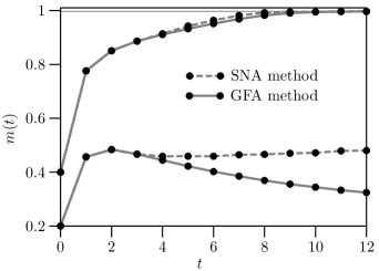
Figure 2: The overlap order parameter as a function of time for the SNA versus the GFA approach for $\alpha=0.1$, $T=0.1$ for retrieval behaviour $m_{0}=0.4$ and spin-glass behaviour $m_{0}=0.2$. The thin line represents the stationary limit for retrieval.

We see that the SNA results coincide with those of the GFA up to the third time step, as shown analytically. For further time steps the results are strongly dependent upon the parameters of the network determining its behaviour: retrieval or spin-glass behaviour. The parameters chosen in Fig. 2 are $\alpha=0.1$, $T=0.1$, and $m_{0}=0.4$ respectively $m_{0}=0.2$. For the first choice (the two upper curves) the system evolves to the retrieval attractor and one observes that there is only a marginal difference between the SNA and GFA method. This confirms the previous observations made in the literature ([12] and references therein). For the second choice (the two lower curves) the initial overlap is too small such that we are outside the basin of attraction for retrieval and, hence, we do not evolve to the attractor (spin-glass behaviour). Here the SNA method, as used in the literature, does not give good results for further time steps. We remark that we have also compared these results with finite size simulations. These simulations are not indicated on the figure because they lie almost exactly on the GFA lines.

5 The SNA revisited

In this section we show how to treat the feedback correlations in the SNA approach correctly. Looking at the definition of the residual overlap at time $t$, i.e.,

$$r_{N}^{\mu}(t)=\frac{1}{\sqrt{N}}\sum_{i=1}^{N}\xi^{\mu}_{i}\sigma_{i}(t)\quad\mu>1\ ,$$ (76)

we want to know how the dependence between spins and patterns evolves in the course of the dynamics.

In general, the local field at a certain time step $h_{i}(t)$ depends on $\xi_{i}^{\mu}$ in two ways. First, there is the correlation through the occurrence of $\xi_{i}^{\mu}$ in the coupling matrix ($J_{ij}$). We call this type of correlations first order correlations because they are the most obvious ones. Second, there may be so-called second order correlations, being correlations with pattern $\xi_{i}^{\mu}$ through the dynamics as a result of feedback. Second order correlations can only appear due to first order correlations earlier in the dynamics. Therefore, extracting the first order correlations at every time step results in a system that does not depend on $\xi_{i}^{\mu}$ anymore.

We define $\delta h_{i}^{\mu}(s)$ by

$$\delta h_{i}^{\mu}(s)=-\frac{1}{N}\sum_{j}\xi_{i}^{\mu}\xi_{j}^{\mu}\sigma_{j}(s)=-\frac{1}{\sqrt{N}}\xi_{i}^{\mu}r^{\mu}(s)\ .$$ (77)

In this way, adding $\delta h_{i}^{\mu}(t)$ removes the first order correlations from the local field at time $t$, i.e.,

$$\tilde{h}_{i}^{\mu}(s)=h_{i}(s)+\delta h_{i}^{\mu}(s)$$ (78)

such that $\tilde{h}_{i}^{\mu}(s)$ only depends on $\xi_{i}^{\mu}$ in second order. Moreover, $\delta h_{i}^{\mu}(s)$ tends to zero as $1/\sqrt{N}$ in the thermodynamic limit, and can therefore be regarded as a perturbation to the field $h_{i}(s)$. We apply this perturbation for all time steps $s<t$ and find

$$\tilde{\sigma}^{\mu}_{i}(t)=\sigma_{i}(t)+\sum_{s=0}^{t-1}\frac{\partial\sigma_{i}(t)}{\partial\tilde{h}_{i}^{\mu}(s)}\Bigg{|}_{\delta h_{i}^{\mu}(s)=0}\delta h_{i}^{\mu}(s)+{\cal O}(1/N)\ ,$$ (79)

where $\tilde{\sigma}^{\mu}_{i}(t)$ is now completely independent of $\xi_{i}^{\mu}$. We rewrite the derivatives by introducing an external field $\theta_{i}(s)$,

$$\frac{\partial\sigma_{i}(t)}{\partial\delta h_{i}^{\mu}(s)}\Bigg{|}_{\delta h_{i}^{\mu}(s)=0}=\frac{\partial\sigma_{i}(t)}{\partial\theta_{i}(s)}\Bigg{|}_{\theta_{i}(s)=0}\ .$$ (80)

Inserting (77) in (79) and using (80) yields

$$\sigma_{i}(t)=\tilde{\sigma}^{\mu}_{i}(t)+\frac{\xi_{i}^{\mu}}{\sqrt{N}}\sum_{s}\frac{\partial\sigma_{i}(t)}{\partial\theta_{i}(s)}\Bigg{|}_{\theta_{i}(s)=0}r^{\mu}(s)+{\cal O}(1/N)\,.$$ (81)

We multiply both sides by $\xi_{i}^{\mu}/\sqrt{N}$ and sum over $i$, so that

$$r_{N}^{\mu}(t)=\frac{1}{\sqrt{N}}\sum_{i}\xi_{i}^{\mu}\tilde{\sigma}^{\mu}_{i}(t)+\sum_{s}\frac{1}{N}\sum_{i}\frac{\partial\sigma_{i}(t)}{\partial\theta_{i}(s)}\Bigg{|}_{\theta_{i}(s)=0}r_{N}^{\mu}(s)+{\cal O}(1/\sqrt{N})$$ (82)

by using the definition of $r^{\mu}_{N}(t)$. We now take the limit $N\to\infty$. By construction, the first term on the r.h.s. is a sum of independent terms and thus converges to a normal distribution with zero mean and variance 1. To the second term we apply the LLN. The result of the limit reads

$$r^{\mu}(t)=\tilde{r}^{\mu}(t)+\sum_{s}G(t,s)r^{\mu}(s)\,.$$ (83)

This recursion relation for $r^{\mu}(s)$ corresponds to (53) by using the substitution $r^{\mu}$ for $\eta$ and $\tilde{r}^{\mu}$ for $\phi$ as in (65). Finally, we insert this relation into the expression (18) of the local field at time $t+1$ leading to, after some algebra, the expression for the exact local field as in equation (3.3) for the GFA. This shows that we have found all feedback correlations.

6 Other architectures

In this section we shortly discuss the application of the SNA approach to other architectures.

For the extremely diluted symmetric architecture one has found an exact solution for the dynamics up to time step $3$ by using a probabilistic method analogous to the SNA [27] and comparing it with the generating functional approach [28]. In this case, the effective local field, starting from the GFA is given by

$$h(t)=\xi\,m(t)+\alpha\sum_{s=0}^{t-1}R(t,s)\,\sigma(s)+\sqrt{\alpha}\eta(t)$$ (84)

with $\eta(t)$ a temporally correlated noise with zero mean and correlation matrix $\boldsymbol{D}$. Hereby,

$$\boldsymbol{D}=\boldsymbol{C}\qquad\qquad\boldsymbol{R}=\boldsymbol{G}\,.$$ (85)

It is clear that, besides the simplification in both the correlations and retarded self-interaction, feedback correlations of arbitrary length survive and make the dynamics as hard to solve as the one of the fully connected model. Hence, a completely analogous discussion as the one before can be made in this case.

For the extremely diluted asymmetric architecture the effective local field in the GFA approach is given by (84), where now

$$\boldsymbol{D}=\boldsymbol{C}\qquad\qquad\boldsymbol{R}=0\,.$$ (86)

Hence, the retarded self-interaction is zero, telling us that the local field at time $t$ does not directly depend on the spins at previous times but only indirectly via the noise. This is precisely the reason why for $\alpha=0$, the short-memory approximation gives the exact answer (see above). It amounts to having a response function of the form (74). Therefore, the SNA describes the correct dynamics. The reason is that for asymmetric dilution the probability to have a loop of finite length tends to zero in the thermodynamic limit [18, 19].

For sequence processing networks the GFA effective local field is given by (84) with

$$\boldsymbol{D}=\sum_{n\geq 0}(\boldsymbol{G}^{\dagger})^{n}\boldsymbol{C}(\boldsymbol{G})^{n}\qquad\qquad\boldsymbol{R}=0$$ (87)

and the situation is analogous to the one for the asymmetrically diluted model in the sense that the retarded self-interaction is zero. Again we have a response function of the form (74) and, hence, the short-memory approximation is exact. This is consistent with and further explains the results in [4] where it has been shown through explicit calculation that the order parameter equations obtained through the GFA are equivalent to those of statistical neurodynamics.

7 Concluding remarks

In this paper we have revisited the signal-to-noise approach for solving the dynamics of the fully connected Little-Hopfield model by comparing it with the exact generating functional analysis. In order to do so we have derived a recursion relation for the effective local field in the generating functional approach. We have shown that the signal-to-noise analysis is a short-memory approximation that is exact up to the third time step. For further time steps, it stays very accurate in the retrieval region but not in the spin-glass region. These results are confirmed by numerical simulations. The application of these methods to other architectures and to sequence processing models has also been discussed.

References

- [1] Galla T, Coolen A C C and Sherrington D 2003 Preprint cond-mat/0303615
- [2] Bollé D, Busquets Blanco J, Shim G M and Verbeiren T 2003 Preprint cond-mat/0304553 (Physica A at Press)
- [3] Coolen A C C 2001 in Handbook of Biological Physics Vol 4, ed. by Moss F and Gielen S (Elsevier Science) 597
- [4] Kawamura M and Okada M 2002 J. Phys. A: Math. Gen. 35 253
- [5] Siggia E D, Martin P C and Rose H A 1973 Phys. Rev. A, 8423
- [6] De Dominicis C 1978 J. Phys. A: Math. Gen. 18 4913
- [7] Rieger H, Schreckenberg M and Zittartz J 1989 Z. Phys. B 74 527
- [8] Horner H, Bormann D, Frick M, Kinzelbach H and Schmidt A 1989 Z. Phys. B 76 381
- [9] Amari S and Maginu K 1988 Neural Networks 1 63
- [10] Okada M 1995 Neural Networks 8 833
- [11] Nishimori H 2001 Statistical Physics of Spin Glasses and Information Processing (Oxford Univ. Press)
- [12] Bollé D 2003 cond-mat/0307104 to appear in Advances in Condensed Matter and Statistical Mechanics ed. by Korutcheva F and Cuerno R (Nova Science Publishers)
- [13] Kinzel W 1985 Z. Phys. B 60 205
- [14] Patrick A E and Zagrebnov V A 1991 J. Phys. A: Math. Gen. 24 3413
- [15] Patrick A E and Zagrebnov V A 1991 J. Stat. Phys. 63 59
- [16] Peretto P 1984 Biol. Cybern. 50 51
- [17] Fontanari J F and Köberle R 1988 J. Physique 49 13
- [18] Derrida B Gardner E and Zippelius A 1987 Europhys. Lett. 4 167
- [19] Kree R and Zippelius A 1991 in Models of neural networks, eds. Domany E van Hemmen J L and Schulten K (Springer, Berlin)
- [20] Nishimori H and Ozeki T 1993 J. Phys. A: Math. Gen. 26 859
- [21] Henkel R D and Opper M 1990 Europhys. Lett. 11 403
- [22] Patrick A E and Zagrebnov V A 1990 J. Phys France 51 1129
- [23] Bollé D, Jongen G and Shim G M 1998 J. Stat. Phys. 91 125
- [24] Horn R A and Johnson C R 1985 Matrix Analysis, Cambridge University Press
- [25] Barkai E, Kanter I and Sompolinsky H 1990 Phys. Rev. A 41 590
- [26] Eissfeller H and Opper M 1992 Phys. Rev. Lett. 68 2094
- [27] Patrick A E and Zagrebnov V A 1992 J. Phys A: Math. Gen. 25 1009
- [28] Watkin T L H and Sherrington D 1991 J. Phys A: Math. Gen. 24 5427