Effect of inhomogeneous magnetic flux on double-dot Aharonov-Bohm Interferometer

Abstract

The influence of the inhomogeneous distribution of the magnetic flux on quantum transport through coupled double quantum dots embedded in an Aharonov-Bohm interferometer are investigated. We show that the effective tunnelling coupling between two dots can be tuned by the magnetic flux imbalance threading two AB subrings. Thus the conductance and the local densities of states become periodic functions of the magnetic flux imbalance. Therefore, transport signals can be manipulated by adjusting the magnetic flux imbalance. Thus accurate control of the distribution of the magnetic flux is necessary for any practical application of such an Aharonov-Bohm interferometer.

I Introduction

Due to recent advances in nanotechnologies, quantum transport through ultra-small quantum dots (QD) has drawn considerable interests in the last decades.books In such small structures with geometrical dimensions smaller than the elastic mean free paths, electron transport is ballistic and its phase coherence can be sustained. To probe the coherence, interference experiments, most notably Aharonov-Bohm (AB) interferometry, are needed. The presence of conductance oscillations as a function of magnetic flux has been experimentally demonstrated for AB interferometers with one QD.Yacobi95 ; Schuster97 ; Ji00 ; Wiel00 ; Kobayashi ; Kobayashi-fano In Ref. Kobayashi-fano, , mesoscopic Fano effect with complex Fano’s asymmetric parameters is observed, and it is shown that Fano effect can be a powerful tool to investigate the electron phase variation in such mesoscopic transport.

Recently, the AB interferometer containing two coupled QD’s with a QD inserted in each arm has also been studied experimentally.holleitner01 ; holleitner02 ; blick03 ; Sigrist03 While there have already been many works for the AB interferometer containing two QD’s, most of them consider only the system without direct coupling between dots. Particular interest in the coupled system lies in its potential application in quantum communication,Loss00 because entanglement of electrons is possible in the presence of direct tunnelling between dots. Just like the molecule of two atoms, two coupled QD’s can form the bonding and antibonding states. Therefore, such an AB interferometer can also be used to probe the phase coherence of the bonding between dots. Moreover, the possibility to control each of two QD’s separately increases the dimension of the parameter space for the transport properties as compared to their single-dot AB counterparts. Thus it can be considered as the starting point of the study for experimentally unexplored region. Motivated by these experimental works, theoretical investigations for such a system have just begun.Jiang02 ; Kang02 It is noted in Ref. Jiang02, that the interdot tunnelling divides the AB interferometer into two coupled subrings, and the total magnetic flux through the device is composed of magnetic flux through two subrings. If the applied magnetic field is non-uniform and/or the construction of the AB interferometer is asymmetric, the magnetic flux threading two subrings can in general be different.note-1 The possibility of non-uniform distribution of magnetic flux is not taken into account in Ref. Kang02, .

In this paper, the AB interferometer containing two coupled QD’s is investigated, and we focus our attention on the effect of inhomogeneous magnetic flux. While this effect has been studied in Ref. Jiang02, by solving numerically the modified rate equations, they consider only a special case with integer values of magnetic flux ratio of two subrings. Our aim is to provide general analytic expressions of the conductance and the local densities of states, which may serve as guides for the ongoing and future experimental endeavor.note-2

By solving exactly a simple model system, we derive general formulas of the conductance and the local densities of states, which includes most of the previous results.Kang02 ; Jiang02 ; Guevara Moreover, we find that non-uniform distribution of the magnetic field piercing the AB interferometer will give an important influence on electrons transport. Thus complex characteristic transport features can occur, which can easily be manipulated by applied gate voltages and magnetic flux. First, the magnetic flux imbalance contributes a phase factor on the tunnelling coupling. Thus the overlapping of the dot’s wave functions can be tuned through the phase of the interdot tunnelling matrix element by adjusting the flux imbalance. Second, the conductance and the local densities of states consist of the Breit-Wigner and the Fano resonances. The corresponding Fano factors, the positions and the widths of these resonances depend not only on the total magnetic flux, but also on the magnetic flux imbalance. Thus electron transport can be controlled by changing both the total magnetic flux and the magnetic flux imbalance. Third, the normal AB oscillations with a period of 2$\pi$ are destroyed, and complex periodic oscillations can be generated. The oscillation periods for the total magnetic flux and the magnetic flux imbalance are in general $4\pi$, while in some particular situations, the $2\pi$-periodicity can be recovered. Besides the $2\pi$ and the $4\pi$-period oscillation, if $\phi$ and $\delta\phi$ are not independent, the oscillating periods can have other possibilities. For the particular case where the ratio of the magnetic flux in two subrings is an integer $n$,Jiang02 the oscillating period becomes $2(n+1)\pi$. All of these results can be easily read off from our general analytic expressions. Furthermore, the AB oscillations can be very sensitive to the magnetic flux imbalance. Thus accurate control of the distribution of the magnetic flux is necessary for any practical application of such an AB interferometer.

The paper is organized as follows. We describe the model in Sec. II. The general expressions of the differential conductance and the density of states are derived there. In Sec. III, we evaluate the conductance as a function of the Fermi energy, and show that the conductance in the present case consists of two resonances which are composed of a Breit-Wigner resonance and a Fano resonance. The local densities of states are calculated in Sec. IV, which show similar behaviors to the conductance. In Sec. V, the AB oscillation of the conductance as a function of total magnetic flux and flux imbalance are studied. Finally, the results are summarized and discussed in Sec. VI. In Sec. III-V symmetric coupling of the dots to the left and right leads is assumed for simplicity. The effect of asymmetric coupling is briefly discussed in Appendix.

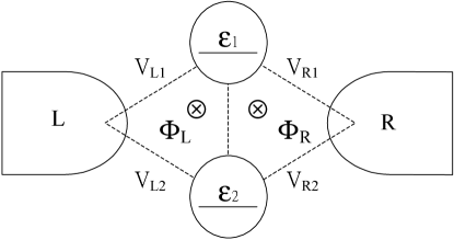
Figure 1: Schematic diagram of two transversely coupled quantum dots embedded in an Aharonov-Bohm interferometer.

II Theory

We consider an AB geometry as depicted in Fig. 1, which is basically equivalent to the experimental setup of Ref. holleitner01, . The interdot and the intradot electron-electron interactions are neglected, and only one energy level in each dot is assumed relevant. The magnetic flux threading the right-handed (left-handed) subring is denoted by $\Phi_{R}$ ($\Phi_{L}$). Thus the total magnetic flux through the whole AB interferometer is $\Phi=\Phi_{L}+\Phi_{R}$. The Hamiltonian of the system can be written as

$$H = \sum_{k\alpha}\varepsilon_{k\alpha}c_{k\alpha}^{\dagger}c_{k\alpha}+{\bf d}^{\dagger}{\bf H}_{0}{\bf d}$$ (1)

$$+\sum_{k\alpha}\left(c_{k\alpha}^{\dagger}{\bf V}_{k\alpha}{\bf d}+{\rm H.c.}\right),$$

where $c_{k\alpha}^{\dagger}$ ($c_{k\alpha}$) are the creation (annihilation) operators for electrons with momentum $k$ in the leads $\alpha=L,R$. For convenience, we introduce the following matrix representation for the dynamics of the isolate double QD’s and the tunnelling between dots and leads:

$${\bf d}^{\dagger}=(d_{1}^{\dagger},d_{2}^{\dagger}),\qquad{\bf d}=\left(\begin{array}[]{c}d_{1}\\ d_{2}\end{array}\right),$$ (4)

$${\bf H}_{0}=\left(\begin{array}[]{cc}\varepsilon_{1}&t\\ t^{*}&\varepsilon_{2}\end{array}\right),$$ (7)

$${\bf V}_{k\alpha}=(V_{k\alpha 1},V_{k\alpha 2}),$$

where $d_{i}$ ($d_{i}^{\dagger}$) annihilates (creates) an electron in $i$-th dot ($i=1,2$). The energy level in dot $i$ is denoted by $\varepsilon_{i}$, which can be varied by the applied gate voltages. $t$ is the interdot tunnelling coupling, and $V_{k\alpha i}$ are the tunnelling matrix elements between dots and leads. The magnetic flux is described by an AB phase factors attached to the interdot tunnelling coupling and the tunnelling matrix elements. We choose a gauge such that $t=|t|\exp(i\delta\phi/2)$, $V_{kL1}=|V_{kL1}|\exp(-i\phi/4)$, $V_{kL2}=|V_{kL2}|\exp(i\phi/4)$, $V_{kR2}=|V_{kR2}|\exp(-i\phi/4)$, and $V_{kR1}=|V_{kR1}|\exp(i\phi/4)$ with the (dimensionless) total magnetic flux $\phi\equiv 2\pi\Phi/\Phi_{0}$ and the (dimensionless) magnetic flux imbalance $\delta\phi\equiv 2\pi(\Phi_{L}-\Phi_{R})/\Phi_{0}$, where $\Phi_{0}=h/e$ is the flux quantum.

By employing the Landauer formula at zero temperature, the differential conductance $G$ is related to the transmission $T(\omega)$ of an electron of energy $\omega$,Meir

$$G=\frac{e^{2}}{h}T(\varepsilon_{F}),$$ (8)

where $\varepsilon_{F}$ stands for the Fermi level of both leads. The total transmission $T(\omega)$ can be expressed as

$$T(\omega)={\rm Tr}\left\{{\bf\Gamma}^{L}{\bf G}^{a}(\omega){\bf\Gamma}^{R}{\bf G}^{r}(\omega)\right\},$$ (9)

where ${\bf G}^{r(a)}(\omega)$ is the Fourier transform of the retarded (advanced) Green’s function of the QD’s, ${\bf G}^{r(a)}(t)=\mp i\theta(\pm t)\langle\{{\bf d}(t),{\bf d}^{\dagger}(0)\}\rangle$, where $\theta(t)$ is the step function and the upper (lower) signs correspond to the retarded (advanced) one. The matrix ${\bf\Gamma}^{\alpha}=2\pi\sum_{k}{\bf V}_{k\alpha}^{\dagger}{\bf V}_{k\alpha}\delta(\omega-\varepsilon_{k\alpha})$ describes the tunnelling coupling of the two QD’s to the lead $\alpha$. Here we neglect the energy dependence of ${\bf\Gamma}^{\alpha}$. Notice that the off-diagonal matrix elements of ${\bf\Gamma}^{\alpha}$ are complex numbers due to the AB phase factors.

By using the equation of motion method, the exact retarded (advanced) Green’s function of the QD’s is given by

$${\bf G}^{r(a)}(\omega)=\frac{1}{D^{r(a)}(\omega)}\left(\begin{array}[]{cc}\omega-\varepsilon_{2}\pm\frac{i}{2}\Gamma_{22}&t\mp\frac{i}{2}\Gamma_{12}\\ t^{*}\mp\frac{i}{2}\Gamma_{21}&\omega-\varepsilon_{1}\pm\frac{i}{2}\Gamma_{11}\end{array}\right),$$ (12)

where

$$D^{r(a)}(\omega) = (\omega-\varepsilon_{1}\pm\frac{i}{2}{\Gamma}_{11})(\omega-\varepsilon_{2}\pm\frac{i}{2}\Gamma_{22})+\frac{1}{4}(|\Gamma^{L}_{12}|^{2}+|\Gamma^{R}_{12}|^{2})$$ (13)

$$+\frac{1}{2}|\Gamma^{L}_{12}||\Gamma^{R}_{12}|\cos\phi-|t|^{2}\mp i|t||\Gamma^{L}_{12}|\cos(\frac{\phi+\delta\phi}{2})\mp i|t||\Gamma^{R}_{12}|\cos(\frac{\phi-\delta\phi}{2})$$

with ${\bf\Gamma}=\sum_{\alpha}{\bf\Gamma}^{\alpha}$. From the above expression, we find that the conductance depends not only on the total magnetic flux $\phi$, but also on the magnetic flux imbalance $\delta\phi$ between the right and the left parts of the present double-dot AB interferometer. As mentioned before, without the interdot tunnelling coupling $|t|=0$, there is only one loop in the AB interferometer, and the transport is determined only by the phase $\phi$. In the special case of zero magnetic field, our result reduces to that obtained in Ref. Guevara, .

From Eqs. (12) and (13), general expressions of the conductance and the local density of states can be reached. However, since we focus our attention on the effect of flux imbalance, we assume for simplicity that the magnitudes of tunnelling matrix elements between the dots and the leads are the same. Thus all of the magnitudes $|\Gamma^{\alpha}_{ij}|$ become identical, which is denoted by $\Gamma/2$, while their values are not the same because of the AB phase factors. (As shown in Appendix, the following results are qualitatively unchanged even when the magnitudes of $|\Gamma^{\alpha}_{ij}|$ are different.) After substituting Eqs. (9)-(13) into Eq. (8), we can obtain a compact form of the differential conductance

$$G=\frac{e^{2}}{h}\frac{(e_{+}-e_{-})^{2}+4\Delta}{|(i-e_{+})(i-e_{-})-\Delta^{\prime}|^{2}}$$ (14)

with

$$e_{\pm} \equiv \frac{2\left(\bar{\varepsilon}\pm|t|\cos\frac{\delta\phi}{2}-\varepsilon_{F}\right)}{\Gamma_{\pm}},$$

$$\Delta \equiv \frac{(\delta\varepsilon)^{2}}{\Gamma_{+}\Gamma_{-}},$$

$$\Delta^{\prime} \equiv \frac{(\delta\varepsilon)^{2}+4|t|^{2}\sin^{2}\frac{\delta\phi}{2}}{\Gamma_{+}\Gamma_{-}},$$ (15)

$$\Gamma_{\pm} \equiv (1\mp\cos\frac{\phi}{2})\Gamma,$$

where $\bar{\varepsilon}\equiv(\varepsilon_{1}+\varepsilon_{2})/2$ and $\delta\varepsilon\equiv\varepsilon_{1}-\varepsilon_{2}$ denote the mean energy and the energy detuning of two QD’s, respectively. The parameters of $e_{+}$ and $\Gamma_{+}$ ($e_{-}$ and $\Gamma_{-}$) are relevant to the antibonding (bonding) state of the QD molecule. From the above result, we find that the conductance shows oscillation patterns when either the total magnetic flux $\phi$ or the magnetic flux imbalance $\delta\phi$ is changed (see also Sec. V). We note that Eq. (14) becomes identical to that obtained in Ref. Kang02, in the special case of $\delta\phi=0$, which will even reduces to the result obtained in Ref. Kubala02, in the case of the absence of the interdot coupling ($t=0$). However, when the distribution of the magnetic flux is non-uniform (i.e., $\delta\phi\neq 0$), more interesting behaviors can show up. It is clear from the expression of $e_{\pm}$ that, by adjusting the phase of the interdot tunnelling matrix element through the flux imbalance $\delta\phi$ in the AB interferometer, one can tune the overlapping of the dot’s wave functions. Moreover, the level crossing of the bonding and the antibonding states can occur by varying $\delta\phi$. We emphasize again that these are possible only when interdot tunnelling coupling is nonzero.

The local density of states at the $i$-th QD is given by $\rho_{i}(\omega)=-{\rm Im}G_{ii}^{r}(\omega)/\pi$. By using the expression of the retarded Green’s function in Eq. (12), the general formula of the local densities of states at $\varepsilon_{F}$ can be written as

$$\rho_{1(2)}(\varepsilon_{F})=\frac{\Gamma_{+}e_{+}^{2}+\Gamma_{-}e_{-}^{2}+(\Gamma_{+}+\Gamma_{-})(1+\Delta^{\prime})\mp 2\;\delta\varepsilon(e_{+}+e_{-})}{2\pi\Gamma_{+}\Gamma_{-}|(i-e_{+})(i-e_{-})-\Delta^{\prime}|^{2}},$$ (16)

where the upper (lower) sign corresponds to $\rho_{1}$ ($\rho_{2}$). Because most of the parameters defined in Eq. (15) depend on $\phi$ and/or $\delta\phi$, the local densities of states $\rho_{1}$ and $\rho_{2}$ again have oscillating behaviors as the total magnetic flux and/or the magnetic flux imbalance are varied.

III conductance

The general form of the conductance in Eq. (14) is quite similar to that obtained in Ref. Kang02, for the $\delta\phi=0$ case. Therefore, following the same kind of analysis, one can easily show that the conductance in the present case consists of two resonances which are composed of a Breit-Wigner resonance and a Fano resonance.

Without loss of generality, we can discuss the case in the limit $\Gamma_{-}\gg\Gamma_{+}$. If the energy scale is larger than $\Gamma_{+}$ ($|e_{+}|\gg 1$), the conductance in Eq. (14) indeed takes the Breit-Wigner form:

$$G\simeq G_{\rm BW}=\frac{e^{2}}{h}\frac{1}{e_{-}^{2}+1}.$$ (17)

Its width is $\Gamma_{-}$ which depends on the total magnetic flux but not on the flux imbalance [see Eq. (15)]. Near the narrower resonance regime $(|e_{+}|\lesssim 1)$, the conductance does show the Fano-resonance behavior,

$$G\simeq G_{\rm Fano}=\frac{e^{2}}{h}T_{b}\frac{|e^{\prime}_{+}+Q|^{2}}{{e^{\prime}_{+}}^{2}+1},$$ (18)

where the background transmission is given by $T_{b}=1/(q^{2}+1)$ with $q=4|t|\cos(\delta\phi/2)/\Gamma_{-}$, and

$$e^{\prime}_{+}=\frac{e_{+}+qT_{b}\Delta^{\prime}}{1+T_{b}\Delta^{\prime}}.$$ (19)

The modified Fano factor is now given by

$$Q=q\frac{1-T_{b}\Delta^{\prime}}{1+T_{b}\Delta^{\prime}}+i\frac{2\sqrt{\Delta}}{1+T_{b}\Delta^{\prime}},$$ (20)

and the width of the Fano resonance becomes $\Gamma^{\prime}_{+}=\Gamma_{+}(1+T_{b}\Delta^{\prime})$. While these results are formally identical to those obtained in Ref. Kang02, , we show that the modified Fano factor, the position and the width of the resonance all depend not only on the total magnetic flux $\phi$, but also on the magnetic flux imbalance $\delta\phi$. Thus transport signals can be manipulated by adjusting both $\phi$ and $\delta\phi$.

For the perfectly symmetrical geometry (i.e, $\delta\varepsilon=0$ and $|\Gamma^{\alpha}_{ij}|$ are all the same) and in the case of zero magnetic field (or more generally $|\cos(\phi/2)|=1$ and $|\cos(\delta\phi/2)|=1$), the width of the Fano resonance becomes zero (or the life time of the antibonding state becomes infinitely long). It is because the antibonding state now becomes totally decoupled to the leads. Therefore, the Fano resonance will disappear in this case. This phenomena had been pointed out a decade ago,Shahbazyan94 which is recently called as a “ghost of Fano resonance”.Guevara We note that this disappearance of the Fano resonance can happen only in this very special case. For example, even for the perfectly symmetrical geometry, the Fano resonance will show up when the magnetic field is turned on (see also Appendix).

To illustrate the above discussions, the differential conductance $G$ as a function of the Fermi energy $\varepsilon_{F}$ is shown in Fig. 2 for various $\delta\phi$ with $|t|/\Gamma=1$, $\delta\varepsilon=0$ (the so-called “covalent limit”), and $\phi=0.3\pi$. Here $\bar{\varepsilon}$ is taken as the zero-energy level. Fig. 2(a) reproduces the topmost one of Fig. 2 in Ref. Kang02, . We find that, as $\delta\phi$ increases from zero to $\pi$, two resonances come closer and closer, and finally two energy level of resonance meet each other when $\delta\phi=\pi$. This can be understood from the expressions of $e_{-}$ and $e^{\prime}_{+}$. Further increase of $\delta\phi$, the Breit-Wigner resonance keeps moving to the positive-energy side, while the Fano resonance goes to the negative-energy side. The resonance levels will move back when $\delta\phi>2\pi$ and the curve for $\delta\phi=0$ is recovered when $\delta\phi$ is increased to $4\pi$. Thus the conductance has in general a period of $4\pi$ for $\delta\phi$ (for further discussions, see Sec. V).

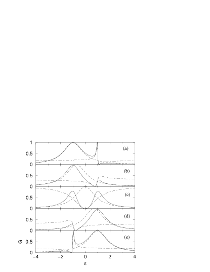
Figure 2: Differential conductance $G$ in unit of $e^{2}/h$ (solid lines) as a function of the Fermi energy (in unit of $\Gamma$) for various flux imbalance. The results shown in panels (a) through (e) correspond to the flux imbalance $\delta\phi=0$, $\pi/2$, $\pi$, $3\pi/2$, and $2\pi$. Other parameters are given by $\bar{\varepsilon}=\delta\varepsilon=0$, $|t|/\Gamma=1$, and $\phi=0.3\pi$. Dashed and dashed-dotted lines denote the Breit-Wigner and the generalized Fano asymptote given in Eq.(17) and Eq.(18), respectively.

In Fig. 2, we find that the zero and the full transmission can occur at some particular values of the Fermi energies. The analytic expressions of these Fermi energies can be easily derived. From Eqs. (14) and (15), it is obvious that, if the two levels of the double QD’s are not the same ($\delta\varepsilon\neq 0$), the conductance cannot be zero. In this case, $\Delta\neq 0$ and the modified Fano factor in Eq. (20) becomes a complex number. It means that the completely destructive interference in the present AB interferometer will not appear in this case. However, when $\delta\varepsilon=0$, the completely destructive interference and transmission zero happen at the Fermi energy

$$\varepsilon_{F}=\bar{\varepsilon}+|t|\cos\frac{\delta\phi}{2}/\cos\frac{\phi}{2},$$ (21)

provided that $\sin(\phi/2)\neq 0$ or $\sin(\delta\phi/2)\neq 0$. It is sensitive to the total magnetic flux $\phi$ and the magnetic flux imbalance $\delta\phi$. On the other hand, the conductance can reach its quantum limit $G=e^{2}/h$ at the Fermi energies

$$\varepsilon_{F}=\bar{\varepsilon}\pm\sqrt{\left(\frac{\delta\varepsilon}{2}\right)^{2}+|t|^{2}-\left(\frac{\Gamma}{2}\right)^{2}\sin^{2}\frac{\phi}{2}}$$ (22)

if $\sin(\phi/2)\sin(\delta\phi/2)=0$ and the expression in the square root is positive. The last term in the square root of Eq. (22) gives the so-called “flux-dependent level attraction” mentioned in Ref. Kubala02, . From the above discussion, it is realized that the value of transmission will in general not be zero or one unless some particular conditions happen to be satisfied.note1

IV local density of states

Similar behaviors to the results in the previous section can be found by examining the local density of states in each of the quantum dots.

For the perfectly symmetrical geometry, $\delta\varepsilon=0$ and $\delta\phi=0$, therefore $\Delta=\Delta^{\prime}=0$, Eq. (16) reduces to

$$\rho_{1}=\rho_{2}=\frac{1}{2\pi\Gamma_{-}(e^{2}_{-}+1)}+\frac{1}{2\pi\Gamma_{+}(e^{2}_{+}+1)}.$$ (23)

That is, both of the local densities of states take the form of the superposition of two Breit-Wigner resonances of widths $\Gamma_{-}$ and $\Gamma_{+}$ at the bonding and antibonding energies, respectively. However, in other cases, following the same kind of analysis in the previous section, it can be shown that the local densities of states consist of a Breit-Wigner at the bonding energy and a Fano line shape at the antibonding energy.

Figure 3: Local density of states at a QD as a function of the Fermi energy (in unit of $\Gamma$). The results shown in panels (a) through (e) correspond to the flux imbalance $\delta\phi=0$, $\pi/2$, $\pi$, $3\pi/2$, and $2\pi$. Other parameters are the same as those used in Fig. 2. Dashed and dashed-dotted lines denote the Breit-Wigner and the generalized Fano asymptote given in Eq.(24) and Eq.(25), respectively.

Without loss of generality, we discuss the case again in the limit $\Gamma_{-}\gg\Gamma_{+}$. If the energy scale is larger than $\Gamma_{+}$ ($|e_{+}|\gg 1$), both of the local densities of states in Eq. (16) take the Breit-Wigner form of width $\Gamma_{-}$:

$$\rho_{1(2)}\simeq\frac{1}{2\pi\Gamma_{-}(e_{-}^{2}+1)}.$$ (24)

Near the narrower resonance regime $(|e_{+}|\lesssim 1)$, the local densities of states show the Fano-resonance behavior,

$$\rho_{1(2)}\simeq\rho_{b}\frac{|e^{\prime}_{+}-P_{1(2)}|^{2}}{1+{e^{\prime}_{+}}^{2}},$$ (25)

where $\rho_{b}\equiv T_{b}/(2\pi\Gamma_{-})$ and the corresponding Fano factor is

$$P_{1(2)}=\frac{qT_{b}\Delta^{\prime}\pm\sqrt{\Delta\frac{\Gamma_{-}}{\Gamma_{+}}}}{1+T_{b}\Delta^{\prime}}+i\frac{\sqrt{\left[\left(q\pm\sqrt{\Delta\frac{\Gamma_{+}}{\Gamma_{-}}}\right)^{2}+(1+\Delta^{\prime}-\Delta)\left(1+\frac{\Gamma_{+}}{\Gamma_{-}}\right)\right]\frac{\Gamma_{-}}{\Gamma_{+}}}}{1+T_{b}\Delta^{\prime}},$$ (26)

where the upper (lower) sign corresponds to $P_{1}$ ($P_{2}$). The Fano factor in Eq. (26) is more complicated than that for the conductance [Eq. (20)]. Thus it is possible in some situations (say, $\Delta=0$) that $P_{1(2)}$ is a complex number but $Q$ is real. Notice that the present Fano factors are in general not the same for different QD’s. From the above results, it can be understood that the Fano factor $P_{1(2)}$, the position and the width of the resonance all can be manipulated by adjusting both of the total magnetic flux $\phi$ and the magnetic flux imbalance $\delta\phi$. In the absence of the magnetic field, the above expressions are equivalent to Eqs. (27) and (28) of Ref. Guevara, .

The local density of states of as a function of Fermi energy $\varepsilon_{F}$ is plotted in Fig. 3 for the same parameters used in Fig. 2. In this case, $\rho_{1}=\rho_{2}$. We find that same level crossing appears as $\delta\phi$ is varied and the curve has again a period of $4\pi$ for $\delta\phi$ (for further discussions, see Sec. V). We notice that the local density of states is always nonvanishing for the chosen parameters, because the Fano factor $P_{1(2)}$ is complex in these cases. As compared with Fig. 2, it is found that the states with small density of states can have almost full transmission and those with large density of states can show zero transmission. This indicates that the full and the zero transmission are indeed consequences of the quantum interference, as mentioned before.

V Aharonov-Bohm Oscillations

We now discuss the AB oscillation of the conductance as a function of total magnetic flux $\phi$ and the magnetic flux imbalance $\delta\phi$ with fixed mean energy $\bar{\varepsilon}$ and energy detuning $\delta\varepsilon$ of two QD’s.

From Eq. (14), it is clear that the conductance [and also the local densities of states, see Eq. (16)] is a periodic function of both $\phi$ and $\delta\phi$. The oscillation periods for $\phi$ and $\delta\phi$ are in general $4\pi$. The $4\pi$-period oscillation for $\delta\phi$ has be implied in Fig. 2, and the $4\pi$-period oscillation for $\phi$ in the case of $\delta\phi=0$ has be found in Ref. Kang02, . However, in the following particular situations, the $2\pi$-periodicity can occur. (i) If we take $\varepsilon_{F}=\bar{\varepsilon}$, then $\Gamma_{+}e_{+}=-\Gamma_{-}e_{-}=2|t|\cos(\delta\phi/2)$. In this case, one can show that the conductance is now a function of $\cos^{2}(\phi/2)$ and $\cos^{2}(\delta\phi/2)$. Hence the conductance shows $2\pi$-period oscillation.note2 This $2\pi$-period oscillation for $\delta\phi$ can be understood from Fig. 2, if we trace the change of $G$ at $\varepsilon_{F}=\bar{\varepsilon}=0$ as $\delta\phi$ is varied from 0 to $2\pi$. (ii) If $\delta\phi=\pi$ [or more generally $\cos(\delta\phi/2)=0$], we have $\Gamma_{+}e_{+}=\Gamma_{-}e_{-}=2\left(\bar{\varepsilon}-\varepsilon_{F}\right)$. Therefore, the conductance becomes a function of $\cos^{2}(\phi/2)$ and the oscillation periods for $\phi$ is $2\pi$. (iii) If $\phi=\pi$ [or more generally $\cos(\phi/2)=0$], we have $\Gamma_{+}=\Gamma_{-}=\Gamma$. In this case, the conductance is a function of $\cos^{2}(\delta\phi/2)$ with a $2\pi$-period oscillation for $\delta\phi$.

As an illustration, the AB oscillation as a function of $\phi$ is shown in Fig. 4 for different values of $\delta\phi$ with $|t|/\Gamma=0.3$ and $\delta\varepsilon/\Gamma=0.1$. Here we choose $\varepsilon_{F}=\bar{\varepsilon}-\sqrt{\left(\delta\varepsilon/2\right)^{2}+|t|^{2}}$, which is the energy for the bonding state when the QD’s are decoupled to the leads. $\bar{\varepsilon}$ is again taken as the zero-energy level for convenience. The curve for $\delta\phi=0$ corresponds to the $A1$ curve in Fig. 4(c) of Ref. Kang02, , where sharp peaks around $\phi=4n\pi$ ($n=0,\pm 1,\pm 2,\dots$) result. It shows that the conductance can be very sensitive to the total magnetic flux $\phi$ for the chosen parameters (say, near $\phi=0$). This opens the possibility to manipulate transport in a nontrivial way by varying the magnetic field. As shown in Fig. 4, we see that this sensitivity can be even strengthened when $\delta\phi$ is present. As $\delta\phi$ increases to $\pi$, the periodicity even changes from $4\pi$ to $2\pi$, as discussed above.

Figure 4: AB oscillations as a function of the total magnetic flux $\phi$ for various flux imbalance $\delta\phi$. (a) $\delta\phi=0$ (solid line), $\pi/2$ (dotted line), $\pi$ (dashed line). (b) $\delta\phi=\pi$ (dashed line), $3\pi/2$ (dotted line), $2\pi$ (solid line). Here the Fermi energy is taken as the energy for the bonding state when the QD’s are decoupled to the leads (see text). Other parameters are given by $\bar{\varepsilon}=0$, $|t|/\Gamma=0.3$, $\delta\varepsilon/\Gamma=0.1$.

Besides the $2\pi$ and the $4\pi$-period oscillation studied above, it is found that, if $\phi$ and $\delta\phi$ are not independent, the oscillating periods can have other possibilities.Jiang02 The authors of Ref. Jiang02, show numerically that the oscillating period will be $2(n+1)\pi$ when $\delta\phi=[(n-1)/(n+1)]\phi$ (or the magnetic flux ratio $\Phi_{L}/\Phi_{R}=n$) with $n$ being integers. This result can be easily explained from our analytic expression of Eq. (14). As $\phi$ being varied from 0 to $2(n+1)\pi$, $\delta\phi$ is increased from 0 to $2(n-1)\pi$, therefore we have $\Gamma_{\pm}\rightarrow\Gamma_{\pm}$, $e_{\pm}\rightarrow e_{\pm}$ ($\Gamma_{\pm}\rightarrow\Gamma_{\mp}$, $e_{\pm}\rightarrow e_{\mp}$), and $\Delta^{\prime}\rightarrow\Delta^{\prime}$ if $n$ is odd (even). This makes $G$ back to its original value. It means that the oscillating period is $2(n+1)\pi$ in this case.

VI Conclusions

In conclusion, we have investigated the influence of the non-uniform distribution of the magnetic flux on quantum transport through coupled double QD’s embedded in an AB interferometer. We show that the effective tunnelling coupling between two dots can be tuned by the magnetic flux imbalance $\delta\phi$ threading two AB subrings. Therefore, the conductance and the local densities of states become periodic functions of $\delta\phi$. Moreover, the conductance and the local densities of states are shown to be composed of a Breit-Wigner resonance and a Fano resonance. The corresponding Fano factors, the positions and the widths of the resonances all depend not only on $\phi$, but also on $\delta\phi$. Thus transport signals can be manipulated by adjusting both $\phi$ and $\delta\phi$. Finally, we point out that the AB oscillations can be very sensitive to $\delta\phi$. Thus accurate control of the distribution of the magnetic flux is necessary for any practical application of such an AB interferometer.

*

Appendix A effect of asymmetric coupling between dots and leads

In this appendix, we devote ourselves to the effect of difference in the matrix elements of $\Gamma^{\alpha}_{ij}$. As an example, we follow the setup which are considered in Ref. Guevara, in the case of zero magnetic field: $\Gamma_{11}^{R}=\Gamma_{22}^{L}\equiv\gamma_{1}$ and $\Gamma_{11}^{L}=\Gamma_{22}^{R}\equiv\gamma_{2}$, and the magnitudes of the off-diagonal matrix elements $|\Gamma_{21}^{L}|=|\Gamma_{12}^{L}|=|\Gamma_{21}^{R}|=|\Gamma_{12}^{R}|\equiv\sqrt{\gamma_{1}\gamma_{2}}$.

In this case, the conductance and the local densities of states are again given by Eq. (14) and (16) respectively, where $e_{\pm}$ and $\Delta^{\prime}$ are identical to those given in Eq. (15), but $\Delta$ and $\Gamma_{\pm}$ now become:

$$\Delta = \left[\frac{2(\gamma_{1}-\gamma_{2})|t|\sin\frac{\delta\phi}{2}-2\sqrt{\gamma_{1}\gamma_{2}}\;\delta\varepsilon\sin\frac{\phi}{2}}{\Gamma_{+}\Gamma_{-}}\right]^{2},$$ (27)

$$\Gamma_{\pm} = (\gamma_{1}+\gamma_{2})\mp 2\sqrt{\gamma_{1}\gamma_{2}}\cos\frac{\phi}{2}.$$ (28)

When $\gamma_{1}=\gamma_{2}\equiv\Gamma/2$, the above expressions reduce to the corresponding ones in Eq. (15). Thus, merely by replacing the functional forms of $\Delta$ and $\Gamma_{\pm}$, the discussions in the text are still applied in this case of asymmetric coupling between dots and leads. From Eq. (28), one finds that, when $\phi=0$, $\Gamma_{+}$ approaches zero as $\gamma_{1}-\gamma_{2}\rightarrow 0$. This result had been pointed out in Ref. Shahbazyan94, . However, for nonzero magnetic field, none of $\Gamma_{\pm}$ will be zero in the limit $\gamma_{1}-\gamma_{2}\rightarrow 0$ as long as $|\cos\frac{\phi}{2}|\neq 1$. Thus the phenomena of a “ghost of Fano resonance”Guevara will not appear when the magnetic field is nonzero.

References

- (1) Mesoscopic Electron Transport, edited by L. L. Sohn, L. P. Kouwenhoven, and G. Schön (Kluwer, Dordrecht,1997); Single Charge Tunnelling, edited by H. Grabert and M. H. Devoret, (Plenum, New York, 1991); D. V. Averin and K. K. Likharev, in Mesoscopic Phenomena in Solids, ed. B. L. Altshuler, P. A. Lee, and R. A. Webb (Elsevier, Amsterdam, 1991), pp. 173-271.
- (2) A. Yacoby, M. Heiblum, D. Mahalu, and H. Shtrikman, Phys. Rev. Lett. 74, 4047 (1995).
- (3) R. Schuster, E. Buks, M. Heiblum, D. Mahalu, V. Umansky, and H. Shtrikman, Nature (London) 385, 417 (1997).
- (4) Y. Ji, M. Heiblum, D. Sprinzak, D. Mahalu, and H. Shtrikman, Science 290, 779 (2000); Y. Ji, M. Heiblum, and H. Shtrikman, Phys. Rev. Lett. 88, 076601 (2002).
- (5) W.G. van der Wiel, S. De Franceschi, T. Fujisawa, J.M. Elzerman, S. Tarucha, and L.P. Kouwenhoven, Science 289, 2105 (2000).
- (6) K. Kobayashi, H. Aikawa, S. Katsumoto, and Y. Iye, J. Phys. Soc. Jpn. 71, L2094-2097 (2002); H. Aikawa, K. Kobayashi, A. Sano, S. Katsumoto, and Y. Iye, cond-mat/0309084.
- (7) K. Kobayashi, H. Aikawa, S. Katsumoto, and Y. Iye, Phys. Rev. Lett. 88, 256806 (2002); cond-mat/0309570.
- (8) A. W. Holleitner, C. R. Decker, H. Qin, K. Eberl, and R. H. Blick, Phys. Rev. Lett. 87, 256802 (2001).
- (9) A. W. Holleitner, R. H. Blick, A. K. Hüttel, K. Eberl, and J. P. Kotthaus, Science 297, 70 (2002).
- (10) R. H. Blick, A. K. Hüttel, A. W. Holleitner, E. M. Höhberger, H. Qin, J. Kirschbaum, J. Weber, W. Wegscheider, M. Bichler, K. Eberl, and J. P. Hotthaus, Physica E 16, 76 (2003).
- (11) M. Sigrist, A. Fuhrer, T. Ihn, K. Ensslin, W. Wegscheider, M. Bichler, cond-mat/0307269; M. Sigrist, A. Fuhrer, T. Ihn, K. Ensslin, S. E. Ulloa, W. Wegscheider, M. Bichler, cond-mat/0308223.
- (12) D. Loss and E.V. Sukhorukov, Phys. Rev. Lett. 84, 1035 (2000).
- (13) Z. T. Jiang, J. Q. You, S. B. Bian, and H. Z. Zheng, Phys. Rev. B 66, 205306 (2002)
- (14) Kicheon Kang and Sam Young Cho, cond-mat/0210009.
- (15) Here we suggest a possible way to adjust experimentally the flux imbalance in the double-dot AB interferometer. Periodic magnetic field with period about one micrometer has been generated by using a regular array of superconductor [H. A. Carmona et al., Phys. Rev. Lett. 74, 3009 (1995)] or micromagnet [P. D. Ye et al., Phys. Rev. Lett. 74, 3013 (1995)]. By covering various periodic magnetic fields with different periods on the top of the sample with the double-dot AB interferometer, one can change to some extent the magnetic flux imbalance threading two subrings.
- (16) For example, our general analytic expressions of the conductance and the local densities of states provide a better fitting formula for the experimental data as long as the flux imbalance is there. The fitting parameter of the flux imbalance can give an indication of the degree of asymmetry in the construction of the AB interferometer.
- (17) M. L. Ladrón de Guevara, F. Claro, and Pedro A. Orellana, Phys. Rev. B 67, 195335 (2003). There are some typographic errors in their Eqs. (9), (10), (14) and (15).
- (18) Y. Meir and N. Wingreen, Phys. Rev. Lett. 68, 2512 (1992); A. P. Jauho, N. S. Wingreen, and Y. Meir, Phys. Rev. B 50, 5528 (1994).
- (19) B. Kubala and J. König, Phys. Rev. B 65, 245301 (2002).
- (20) T. V. Shahbazyan and M. E. Raikh, Phys. Rev. B 49, 17 123 (1994).
- (21) Similar expressions of the Fermi energies corresponding to the zero and the full transmission have be given in Refs. Guevara, and Kubala02, for various limiting cases. By taking and , Eq. (22) reduces to the condition of full transimission given in Ref. Kubala02, . On the other hand, when the magnetic field is absent and the setup is perfectly symmetrical, i.e., and , Eqs. (21) and (22) can be related to those in Ref. Guevara, .
- (22) In this case, the total density of states, , has also oscillating periods for and . However, the oscillating periods for and of the local densities of states, and , are still unless (i.e., the enrrgy detuning ).