Spin-Flip Noise in a Multi-Terminal Spin-Valve

Abstract

We study shot noise and cross correlations in a four terminal spin-valve geometry using a Boltzmann-Langevin approach. The Fano factor (shot noise to current ratio) depends on the magnetic configuration of the leads and the spin-flip processes in the normal metal. In a four-terminal geometry, spin-flip processes are particular prominent in the cross correlations between terminals with opposite magnetization.

The discovery of the giant magneto resistance effect in magnetic multi-layers has boosted the interest in spin-dependent transport in the last years (for a review see e.g. bauer:97 ). In combination with quantum transport effects the field is termed spintronics prinz:98 . In recent experiments spin-dependent transport in metallic multi-terminal structures has also been demonstrated jedema:00 . One important aspect of quantum transport is the generation of shot noise in mesoscopic conductors blanter:00 ; nazarov:03 . Probabilistic scattering in combination with Fermionic statistics leads to a suppression of the shot noise from its classical value khlus:87 ; lesovik:89 ; buettiker:90 .

A particular interesting phenomenon are the nonlocal correlations between currents in different terminals of a multi-terminal structure. For a non-interacting fermionic system the cross correlations are generally negative buettiker:92 . In a one-channel beam splitter the negative sign was confirmed experimentally henny:99 ; oliver:99 . If the electrons are injected from a superconductor, the cross correlations may change sign and become positive martin:96 ; boerlin:02 ; samuelsson:02 ; taddei:02 . In these studies, however, the spin was only implicitly present due to the singlet pairing in the superconductor.

Current noise in ferromagnetic - normal metal structures, in which the spin degree of freedom plays an essential role, has so far attracted only little attention. Non-collinear two-terminal spin valves have been studied in brataas:02 and it was shown that the noise depends on the relative magnetization angle in a different way than the conductance. Thus, the noise reveals additional information on the internal spin-dynamics. Noise has been exploited to study the properties of localized spins by means of electron spin resonanceengel:00 . Quantum entanglement of itinerant spins can also be probed through noise measurements loss:00 .

In this work we propose a new instrument for the study of spin-dependent transport: the use of cross correlations in a multi-terminal structure. The basic idea is to use a four-terminal structure like sketched in Fig. 1. An electron current flows from the left terminals to the right terminals and is passing a scattering region. In the absence of spin-flip scattering the currents of spin-up electrons and spin-down electron are independent, and the cross correlations between any of the two currents in different spin channels vanish. However, spin-flip scattering can convert spin-up into spin-down electrons and vice versa, and induces correlations between the different spin currents. This has two effects. First, the equilibration of the spin-populations leads to a weakened magneto-resistance effect. Second, the current cross correlations between the differently polarized terminals contain now information on the spin-flip processes taking place in the scattering region.

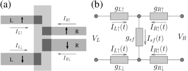
Figure 1: Four-terminal setup to measure spin-flip correlations. (a) a possible experimental realization with a normal diffusive metal strip, on which four ferromagnetic strips are deposited (of different width to facilitate different magnetization orientations). The total length of the diffusive metal underneath the ferromagnetic contacts should be less that the spin-diffusion length in the normal metal. (b) theoretical model of the device. Spin $\uparrow(\downarrow)$ current is flowing in the upper(lower) branch. Spin-flip scattering connects the two spin-branches and is modelled as resistor with also induces additional flutuation.

To this end we will study a four-terminal structure, in which the currents can be measured in all four terminals independently. The layout is shown in Fig. 1, in which the various currents are defined. For simplicity, we assume that all four terminals are coupled by tunnel junctions to one node. The node is assumed to have negligible resistance, but provides spin-flip scattering. The ferromagnetic character of the terminals is modelled by spin-dependent conductances of the tunnel junctions. The two left(right) terminals have chemical potential $V_{1}(V_{2})$. In most of the final results we will assume zero temperature, but this is not crucial. Furthermore, we will assume fully polarized tunnel contacts, characterized by $g_{a\sigma}$, where $a=L,R$ denotes left and right terminals, and $\sigma=\uparrow,\downarrow$ stands for the spin directions (in equations we take $\uparrow=+1$ and $\downarrow=-1$).

The current fluctuations in our structure can be described by a Boltzmann-Langevin formalism nagaev:92 . The time-dependent currents at energy $E$ through contact $a\sigma$ are written as

$$I_{a\sigma}(t,E) = g_{a\sigma}\left[f_{a\sigma}(E)-f_{c\sigma}(E)-\delta f_{c\sigma}(t,E)\right]$$ (1)

$$+\delta I_{a\sigma}(t,E)\,.$$

The averaged occupations of the terminals are denoted by $f_{a\sigma}(E)$, the one of the central node by $f_{c\sigma}(E)$. The occupation of the central node is fluctuating as $\delta f_{c\sigma}(t,E)$. The Langevin source $\delta I_{a\sigma}(t,E)$ induces fluctuations due to the probabilistic scattering in contact $a\sigma$. We assume elastic transport in the following, so all equations are understood to be at the same energy E. Since we assume tunnel contacts, the fluctuations are Poissonian and given by blanter:00

$$\langle\delta I_{a\sigma}(t)\delta I_{a^{\prime}\sigma^{\prime}}(t^{\prime})\rangle=$$ (2)

$$g_{a\sigma}\delta_{\sigma\sigma^{\prime}}\delta_{aa^{\prime}}\delta(t-t^{\prime})\left[f_{a\sigma}+f_{c\sigma}-2f_{a\sigma}f_{c\sigma}\right]\,.$$

The brackets $\langle\cdots\rangle$ denote averaging over the fluctuations. The conservation of the total current at all times $t$ leads to the conservation law displace

$$\sum_{a,\sigma}I_{a\sigma}(t)=0$$ (3)

The equation presented so far describe the transport of two unconnected circuits for spin-up and spin-down electrons, i.e. the spin current is conserved in addition to the total current. Spin-flip scattering on the dot leads to a non-conserved spin current, which we write as

$$\sum_{a,\sigma}\sigma I_{a\sigma}(t) = 2g_{sf}\left[f_{c\uparrow}+\delta f_{c\uparrow}(t)-f_{c\downarrow}-\delta f_{c\downarrow}(t)\right]$$ (4)

$$+2\delta I_{sf}(t)\,.$$

Here we introduced a phenomenological spin-flip conductance $g_{sf}$, which connects the two spin occupations on the node. Correspondingly, we added an additional Langevin source $\delta I_{sf}(t)$, which is related to the probabilistic spin scattering and has a correlation function malek

$$\langle\delta I_{sf}(t)\delta I_{sf}(t^{\prime})\rangle = g_{sf}\delta(t-t^{\prime})$$

$$\times\left[f_{c\uparrow}(1-f_{c\downarrow})+f_{c\downarrow}(1-f_{c\uparrow})\right]\,.$$

Eqs. (1)-(Spin-Flip Noise in a Multi-Terminal Spin-Valve) form a complete set and determine the average currents and the current noise of our system. Solving for the average occupations of the node we obtain

$$f_{c\sigma} = \left[\left(g_{-\sigma}g_{L\sigma}+g_{sf}g_{L}\right)f_{L}\right.$$

$$+\left.\left(g_{-\sigma}g_{R\sigma}+g_{sf}g_{R}\right)f_{R}\right]/Z\,.$$

Here we introduced $g_{\sigma}=g_{L\sigma}+g_{R\sigma}$, $g_{L(R)}=g_{L(R)\uparrow}+g_{L(R)\downarrow}$, and $Z=g_{\uparrow}g_{\downarrow}+(g_{\uparrow}+g_{\downarrow})g_{sf}$. The average currents are then

$$I_{L\sigma}=\frac{g_{L\sigma}}{Z}\left[g_{R\sigma}g_{-\sigma}+g_{R}g_{sf}\right](f_{L}-f_{R})\,,$$ (7)

and the currents through the right terminals are obtained by interchanging $R\leftrightarrow L$ in Eq. (7). The fluctuating occupations on the node are

$$\delta f_{c\sigma}(t) = \left[\left(g_{-\sigma}+g_{sf}\right)\delta I_{\sigma}(t)\right.$$

$$+\left.g_{sf}\delta I_{-\sigma}(t)+g_{-\sigma}\sigma\delta I_{sf}(t)\right]/Z\,,$$

where we introduced $\delta I_{\sigma}(t)=\delta I_{1\sigma}(t)+\delta I_{-1\sigma}(t)$. The total fluctuations of the current in a terminal are obtained from $\Delta I_{a\sigma}(t)=\delta I_{a\sigma}(t)-g_{a\sigma}\delta f_{c\sigma}(t)$ and we find

$$\Delta I_{L\sigma} = \frac{1}{Z}\left[\left(g_{R\sigma}g_{-\sigma}+\left(g_{-\sigma}+g_{R\sigma}\right)g_{sf}\right)\delta I_{L\sigma}\right.$$ (9)

$$-g_{L\sigma}\left(g_{-\sigma}+g_{sf}\right)\delta I_{R\sigma}+\sigma g_{L\sigma}g_{-\sigma}\delta I_{sf}$$

$$\left.-g_{L\sigma}g_{sf}\left(\delta I_{L-\sigma}+\delta I_{R-\sigma}\right)\right]\,.$$

Now we can calculate all possible current correlators in the left terminals, defined by

$$S_{L\sigma\sigma^{\prime}} = \int_{-\infty}^{\infty}d\tau\langle\Delta I_{L\sigma}(t+\tau)\Delta I_{L\sigma^{\prime}}(t)\rangle\,.$$ (10)

The total current noise in the left terminals is

$$S_{L}=S_{L\uparrow\uparrow}+S_{L\downarrow\downarrow}+2S_{L\uparrow\downarrow}\,.$$ (11)

Of course the same quantities can be calculated for the right terminals. From particle conservation it follows that $S_{L}=S_{R}$, but in the presence of spin-flip scattering the individual correlators can differ. For convenience we also define a Fano factor $F=S_{L}/e|I|$, where $I=I_{L\uparrow}+I_{L\downarrow}$ is the total current.

We will discuss general results below, but first concentrate on simple limiting cases. We will restrict ourselves to zero temperature from now on. Assuming a bias voltage $V$ is applied between the right and the left terminals, the occupations are $f_{L}=1$ and $f_{R}=0$ in the energy range $0\leq E\leq eV$. The full current noise can be written as

$$S_{L} = \frac{\left|eV\right|}{Z^{3}}\sum_{\sigma=\uparrow\downarrow}\left[g_{L\sigma}(g_{sf}g_{R}+g_{-\sigma}g_{R\sigma})^{3}\right.$$

$$+g_{R\sigma}(g_{sf}g_{L}+g_{-\sigma}g_{L\sigma})^{3}$$

$$+\frac{g_{sf}}{Z}(g_{\downarrow}g_{L\uparrow}-g_{\uparrow}g_{L\downarrow})^{2}(g_{sf}g_{R}+g_{\sigma}g_{R-\sigma})$$

$$\left.\times(g_{sf}g_{L}+g_{-\sigma}g_{L\sigma})\right]\,.$$

For the cross correlations at the left side we find

$$S_{L\uparrow\downarrow} = -g_{sf}\left|eV\right|\frac{g_{L\uparrow}g_{L\downarrow}}{Z^{3}}\sum_{\sigma=\uparrow\downarrow}$$

$$\big{\{}\left[g_{-\sigma}g_{R\sigma}+(g_{-\sigma}+g_{R\sigma})g_{sf}\right](g_{sf}g_{R}+g_{-\sigma}g_{R\sigma})$$

$$-g_{R\sigma}(g_{-\sigma}+g_{sf})(g_{-\sigma}g_{L\sigma}+g_{sf}g_{L})$$

$$+\frac{g_{\downarrow}g_{\uparrow}}{Z}(g_{-\sigma}g_{L\sigma}+g_{sf}g_{L})(g_{\sigma}g_{R-\sigma}+g_{sf}g_{R})\big{\}}\,.$$

It can be shown, that the cross correlations are always negative, as it should bebuettiker:92 .

In the case of a two-terminal geometry two different configurations are possible. Either both terminals have the same spin-direction, or the opposite configuration. In the first case we can take $g_{\downarrow}=0$. There is no effect of the spin-flip scattering and we obtain for the Fano factor $F=(g_{L}^{2}+g_{R}^{2})/(g_{L}+g_{R})^{2}$, in agreement with the known results blanter:00 . If the two terminals have different spin orientations (’antiferromagnetic’ configuration), the situation is completely different, since transport is allowed only by spin-flip scattering. We take $g_{L\downarrow}=g_{R\uparrow}=0$. The Fano factor is

$$F=1-2g_{sf}g_{L}g_{R}\frac{(g_{L}+g_{R})(g_{L}+g_{sf})(g_{R}+g_{sf})}{(g_{L}g_{R}+(g_{L}+g_{R})g_{sf})^{3}}\,,$$ (14)

where we have used the result for the mean current $I=g_{sf}g_{L}g_{R}/(g_{L}g_{R}+(g_{L}+g_{R})g_{sf})$. The Fano factor, given in Eq. (14) interpolates between the Poisson limit $F=1$ for $g_{sf}\ll g_{L}+g_{R}$ and the result for the double barrier junction $F=(g_{L}^{2}+g_{R}^{2})/(g_{L}+g_{R})^{2}$ for $g_{sf}\gg g_{L}+g_{R}$, coinciding with two-terminal ’ferromagnetic’ configuration mish-prep .

Let us now turn the four-terminal structure and study the effect of spin-flip scattering on the spin cross correlation in lowest order in $g_{sf}/(g_{\uparrow}+g_{\downarrow})$. The zero-frequency cross-correlation between the currents in the left terminals gives

$$\frac{S_{L\uparrow\downarrow}}{|eV|}=-2g_{sf}\frac{g_{L\uparrow}g_{L\downarrow}}{g_{\uparrow}^{2}g_{\downarrow}^{2}}\left[g_{R\uparrow}g_{R\downarrow}+\frac{(g_{L\downarrow}g_{R\uparrow}-g_{L\uparrow}g_{R\downarrow})^{2}}{g_{\uparrow}g_{\downarrow}}\right]\,.$$ (15)

The first term is also present in a spin-symmetric situation, and is caused by the additional current path opened by the spin-flip scattering. The second term in the Eq. (15) depends on the amount of spin accumulation on the central metal, i.e. is proportional to $(f_{c\uparrow}-f_{c\downarrow})^{2}$.

We first consider the symmetric ’ferromagnetic’ configuration $g_{L\uparrow}=g_{R\uparrow}=g_{\uparrow}/2$ and $g_{L\downarrow}=g_{R\downarrow}=g_{\downarrow}/2$. Note, that also $g_{L}=g_{R}$ follows in this configuration. The Fano factor of the full current noise is $F=1/2$, i. e. we recover the usual suppression of the shot noise characteristic for a symmetric double barrier structure. There is no spin accumulation in this configuration, and, consequently, no effect of the spin-flip scattering on the Fano factor. The cross correlations in the ’ferromagnetic’ configuration are

$$S_{L\uparrow\downarrow} = -\frac{g_{sf}}{8}\frac{g_{\uparrow}g_{\downarrow}}{g_{\uparrow}g_{\downarrow}+g_{sf}(g_{\uparrow}+g_{\downarrow})}|eV|\,.$$ (16)

Thus, in the limit of strong spin-flip scattering the cross correlations become independent on $g_{sf}$.

Figure 2: Cross correlations, Fano factor and average currents (symmetric case). We assume symmetric contacts $g_{L}=g_{R}$ and parametrize the magnetic properties with the spin polarization $p_{L(R)}=(g_{L(R)\uparrow}-g_{L(R)\downarrow})/(g_{L(R)\uparrow}+g_{L(R)\downarrow})$. The upper part shows the Fano factor of the current fluctuations in the left contacts for different polarization configurations. Inset: average current. The lower part shows the spin-flip induced cross correlations between $\uparrow$- and $\downarrow$-currents in the left terminals.

Next we consider the symmetric ’antiferromagnetic’ configuration $g_{L\uparrow}=g_{R\downarrow}=g_{1}$ and $g_{L\downarrow}=g_{R\uparrow}=g_{2}$. The Fano factor is

$$F=\frac{1}{2}\left[1-\frac{(g_{1}-g_{2})^{2}}{(g+2g_{sf})^{2}}\left(\frac{2g_{sf}^{2}}{gg_{sf}+2g_{1}g_{2}}-\frac{g}{g+2g_{sf}}\right)\right]\,.$$ (17)

The second term in the brackets in Eq. (17) can be either positive or negative. In the latter case $F$ drops below the symmetric double barrier value of 1/2. For the cross correlations we obtain

$$\frac{S_{L\uparrow\downarrow}}{|eV|} = -\frac{g_{sf}g_{1}g_{2}}{2g^{2}(g+2g_{sf})^{4}}\left[g(g+2g_{sf})^{3}\right.$$ (18)

$$\left.+(g_{1}-g_{2})^{2}\left(3g^{2}+6gg_{sf}+4g_{sf^{2}}\right)\right]\,,$$

where we introduced the abbreviation $g=g_{1}+g_{2}$. Again, the second term in the brackets in Eq. (18) is proportional to the spin accumulation of the island, which enhances the spin-flip induced cross correlations.

The transport properties for symmetric junctions are shown in Fig. 2. For equal polarizations of both sides there is no effect of spin-flip scattering on the Fano factor and average currents. However, the cross correlations do depend on the polarizations even in this case. For small $g_{sf}$ the cross correlations rapidly increase in magnitude. For $g_{sf}\gg g_{L}+g_{R}$ the cross correlations become independent of the relative polarizations. Their absolute value, however, depends strongly on the absolute value of the polarization. For antiparallel polarizations the Fano factor differs strongly from its value 1/2 in the unpolarized case. With increasing spin-flip scattering rate, the Fano factor goes from a value larger than 1/2 through a minimum, which is always lower that 1/2.

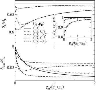
Figure 3: Cross correlations, Fano factor and average currents (asymmetric case). We take here $g_{L}=4g_{R}$. The definition of the polarizations are taken over from Fig. 2.

Let us now turn to the general case of asymmetric junctions. The noise correlations are plotted in Fig. 3. We have taken $g_{L}=4g_{R}$ and various configurations of the polarizations $0.3$ and $0.7$. The Fano factors and the average currents are now different for all parameter combinations. However, the variations of the Fano factors are small, i. e. they are alway close to the unpolarized case. This is different for the cross correlations. Even for weak spin-flip scattering they change dramatically if some of the polarizations are reversed.

In conclusion we have suggested to use shot noise and cross correlations as a tool to study spin-flip scattering in mesoscopic spin-valves fourterm . In a two-terminal device with antiferromagnetically oriented electrodes spin-flip scattering leads to a transition from full Poissonian shot noise (Fano factor $F=1$) to a double-barrier behaviour ($F=1/2$) with increasing spin-flip rate. We have proposed to measure the spin correlations induced by spin-flips in a four-terminal device. If the spin-flip scattering rate is small, the cross-correlation beween currents in terminal with opposite spin-orientation gives direct access to the spin-flip scattering rate. Presently, we have assumed fully polarized terminals, but a generalization to arbitrary polarizations is straightforward.

We acknowledge discussion with C. Bruder. W. B. was financially supported by the Swiss NSF and the NCCR Nanoscience. M. Z. thanks the University of Basel for hospitality. During preparation of this manuscript, a work appeared, in which a similar model was studied sanchezprep .

References

- (1) M. A. M. Gijs and G. E. W. Bauer, Adv. Phys. 46, 285 (1997).
- (2) G. A. Prinz, Phys. Today 282, 1660-1663 (1998); S. Datta and B. B. Das, Appl. Phys. Lett. 56, 665 (1990); J. M. Kikkawa, D. D. Awschalom, Nature 397, 139 (1999); R. Fiederling et al., Nature 402, 787 (2000); Y. Ohno et al., Nature 402, 790 (2000); I. Malajovich et al., Phys. Rev. Lett. 84, 1015 (2000).
- (3) F. J. Jedema et al., Nature 410, 345 (2000); Nature 416, 713 (2002).
- (4) Ya. M. Blanter and M. Büttiker, Phys. Rep. 336, 1 (2000).
- (5) Quantum Noise in Mesoscopic Physics, ed. by Yu. V. Nazarov, Yu. V. (Kluwer, Dordrecht, 2003).
- (6) V. A. Khlus, Sov. Phys. JETP 66, 1243 (1987).
- (7) G. B. Lesovik, JETP Lett. 49, 592 (1989).
- (8) M. Büttiker, Phys. Rev. Lett. 65, 2901 (1990).
- (9) M. Büttiker, Phys. Rev. B 46, 12485 (1992).
- (10) M. Henny et al., Science 284, 296 (1999); S. Oberholzer et al., Physica (Amsterdam) 6E, 314 (2000).
- (11) W. D. Oliver et al., Science 284, 299 (1999).
- (12) T. Martin, Phys. Lett. A 220, 137 (1996); M. P. Anantram and S. Datta, Phys. Rev. B 53, 16390 (1996); G. B. Lesovik, T. Martin, and J. Torreś, Phys. Rev. B 60, 11935 (1999). J. Torres and T. Martin, Eur. Phys. J. B 12, 319 (1999).
- (13) J. Börlin, W. Belzig, and C. Bruder Phys. Rev. Lett. 88, 197001 (2002).
- (14) P. Samuelsson and M. Büttiker, Phys. Rev. Lett. 89, 046601 (2002).
- (15) F. Taddei and R. Fazio, Phys. Rev. B 65, 134522 (2002).
- (16) Y. Tserkovnyak and A. Brataas, Phys. Rev. B 64, 214402 (2001).
- (17) H.-A. Engel and D. Loss, Phys. Rev. B 65, 195321 (2002).
- (18) D. Loss and E. V. Sukhorukov, Phys. Rev. Lett. 84, 1035 (2000); G. Burkard, D. Loss, and E. V. Sukhorukov, Phys. Rev. B 61, R16303 (2000); J. C. Egues, G. Burkard, and D. Loss, Phys. Rev. Lett. 89, 176401 (2002).
- (19) K. E. Nagaev, Phys. Lett. A 169, 103 (1992); Phys. Rev. B 57, 4628 (1998).
- (20) In our calculation we neglect all charging effects, i. e. we assume that . We are also only interested here in current fluctuations on time-scales longer than all -times.
- (21) M. Zareyan and W. Belzig (unpublished).
- (22) A similar effect was recently reported in E. G. Mishchenko, cond-mat/0305003 (unpublished).
- (23) The four-terminal structure suggested in Fig. 1(a) is particularly suitable. Without applying an external magnetic field the magnetic configuration can be switched by changing the potentials of the different terminals.
- (24) D. Sanchéz et al., cond-mat/0306132 (unpublished).