Semiclassical analysis and the magnetization of the Hofstadter model

Abstract

The magnetization and the de Haas-van Alphen oscillations of Bloch electrons are calculated near commensurate magnetic fluxes. Two phases that appear in the quantization of mixed systems—the Berry’s phase and a phase first discovered by Wilkinson—play a key role in the theory.

The magnetization of a free electron gas was calculated by L. Landau in 1930 in the early days of quantum mechanics [1]. Considerable efforts have since been devoted to extending Landau results to Bloch electrons, i.e., in the presence of periodic background potential. Most of the efforts and progress made was in the region of weak magnetic fields [2, 3] where the flux $\Phi$ through a unit cell is small. This is adequate for most solid state applications. There is, however, also considerable interest in a better understanding of phenomena that have to do with commensuration in condensed matter physics [4, 5, 6, 7, 8]. This is the case when $\Phi$ is close to a rational number. The magnetization of Bloch electrons near rational fluxes, other than $\Phi=0$, remained an open challenge which we solve here. The difficulty lies in the delicate spectral properties resulting from commensuration [5]. The Hofstadter model is a basic model for a system where commensuration plays a role. It is also a basic paradigm for a quantum system with fractal spectra [6], anomalous quantum transport [7] and the (integer) quantum Hall effect [9].

The problem of magnetization near fractional flux becomes tractable by an idea that goes back to M. Wilkinson [8]. Namely, that near a rational flux the Hamiltonian can be understood as the semiclassical quantization of a mixed system: In mixed systems some, but not all, degrees of freedom may be treated semiclassically. As a consequence the “classical Hamiltonian” is matrix (or operator) valued. Pauli and Dirac equations for a spinning electron in a slowly varying potential, the Born-Oppenheimer theory of molecules, and the Hofstadter model near rational flux [8] are examples of mixed systems. In the Hofstadter model the role of the Planck constant is played by the deviation from a nearby rational

$$h=\Phi-\frac{p}{q}\ .$$ (1)

Littlejohn and Flynn [10] developed an elegant geometric formalism for the quantization of mixed systems. They show that in order $\hbar$ the quantization of mixed systems gives rise to two phases: One is the Berry’s phase [11] and the other is a phase that is sometimes known as the “no-name phase” [12] and sometimes as the Wilkinson-Rammal (WR) phase [13]. For both phases to appear, the “classical Hamiltonian” must have non-trivial commutation properties in both coordinates and momenta. These phases play a central role in determining the magnetization, see e.g. Eq. (25) below.

Our results are closely related to recent progress made in the semiclassical dynamics of Bloch electrons under slowly varying electric and magnetic fields [13]. When one goes beyond the leading order expressed by Peierls substitution [2, 13] one finds that the Berry’s phase and the WR phase play a role in the dynamics. This lead [13] to identify the WR term with the magnetization of a wave packet. Although related, the notions of wave packet vs. thermodynamic magnetization, expressed in Eq. (25), are distinct; for example, wave packet magnetization is not defined in the gaps, while the thermodynamic magnetization and, of course, the de Haas van Alphen oscillations, have a non-trivial dependence on the chemical potential also in the gaps.

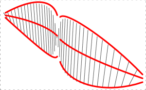
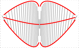
Figure 1: The de Haas van-Alphen oscialltions of the magnetization as a function of the chemical potential in the Hofstadter model for flux $\Phi=40/121$, compared with the limiting envelopes and their averages, and the gap magnetization for $\Phi\to 1/3$. The two insets are details of the left and center envelopes.

Fig. 1 shows the zero temperature magnetization at $\Phi=\frac{1}{3+\frac{1}{40}}$. The complexity of the magnetization is due to the multiplicity of scales: The big scale is determined by the denominator $q=3$, and the small scale by $h$. On the small scale one sees the rapid de Haas-van Alphen oscillations. On the big scales one sees continuous features: the linear pieces in the (big) gaps, the envelopes of the de Haas-van Alphen oscillations and their mean. Our theory of magnetization accounts for all these features.

We show that while the amplitude of the oscillation is determined solely by the leading terms in the semiclassical expansion, the mean magnetization requires knowledge of the terms beyond leading order, thus depending on the fine details of the spectrum. Intriguingly, it is the latter quantity which is stable against perturbations. Finite temperatures larger than the typical eigenvalue spacing wash out the de Haas-van Alphen oscillations of the small scale but leave intact the mean magnetization. Semiclassical approximations that retain only the leading order yield no magnetization at all at finite temperatures.

Let us start by describing the semiclassical quantization of mixed systems [10]. The “classical Hamiltonian”, ${\cal H}(x,k)$, is a Hermitian matrix which depends on $x$ and $k$. We shall denote by $\varepsilon_{j}(x,k)$ its $j$-th band of eigenvalues and by $\left|u_{j}(x,k)\right\rangle$ the corresponding eigenvectors. We shall also assume that bands do not cross. The corresponding quantum Hamiltonian is ${\cal H}(\hat{x},\hat{k})$ with $[\hat{x},\hat{k}]=i\hbar$.

Let $S(E;H,{\rho})$ denote the classical action associated with a closed orbit of energy $E$ of a classical Hamiltonian function $H$, with phase space area form ${\rho}$. Since phase space is two dimensional the action is the area enclosed by the orbit. Note that $H$, unlike ${\cal H}$, is a scalar valued function. The Bohr-Sommerfeld quantization rule in mixed systems says that the semiclassical approximation of the eigenvalue $E_{n}$ is given by

$$S(E_{n};H_{\hbar},{\rho}_{\hbar})=h\,(n+\gamma_{m})\ ,\quad n\in\mathbb{Z}$$ (2)

where $\gamma_{m}$, is the Maslov index of the orbit [14]. $H_{\hbar}$ has an expansion in powers of $\hbar$, $H_{\hbar}=H^{(0)}+\hbar H^{(1)}+\cdots\,$. Peierls substitution sets $H_{j}^{(0)}(x,k)=\varepsilon_{j}(x,k)$, and the next order is [10]

$$H_{j}^{(1)}(x,k)={\rm Im}\left\langle\partial_{x}u_{j}\right|({\cal H}-\varepsilon_{j})\left|\,\partial_{k}u_{j}\right\rangle(x,k)\ .$$ (3)

The expansion ${\rho}_{\hbar}={\rho}^{(0)}+\hbar{\rho}^{(1)}+\cdots$ begins with the canonical form ${\rho}_{j}^{(0)}=dk\wedge dx$ and the subleading term is the Berry curvature form

$${\rho}_{j}^{(1)}=2\omega(x,k)\,dk\wedge dx\ ,\quad\omega(x,k)={\rm Im}\left\langle\partial_{x}u_{j}\right|\partial_{k}{u_{j}}\rangle(x,k)\ .$$ (4)

This formulation is manifestly gauge invariant (independent of the choice of phases for $\left|u_{j}\right\rangle$) and preserves the symmetry properties of $\cal H$, which is useful when one wants to correctly count the dimension of the Hilbert space of the quantized operator, as we now proceed to explain.

Suppose that $\cal H$ is periodic in both $x$ and $k$ up to gauge transformations, and hence describes (classical) motion on a phase space torus $\cal T$. $H_{j}^{(0)}$, $H_{j}^{(1)}$ and ${\rho}_{j}^{(1)}$ are all well-defined functions on $\cal T$. The Chern number of the $j$-th band is the integer

$$C_{j}=\frac{1}{\pi}\int_{\cal T}\,\omega_{j}\,dk\wedge dx$$ (5)

It follows from Eqs. (2,4) that the dimension of the Hilbert space associated with the $j$-th band is

$$\frac{|{\cal T}|}{h}+C_{j}\ ,$$ (6)

where $|{\cal T}|$ denotes the area of $\cal T$. Since the dimension of the Hilbert space is necessarily an integer, quantization on the torus is possible only for certain values of $h$. Eq. (6) goes beyond the classical Weyl law which only determines the leading, $|{\cal T}|/h$, behavior. The Chern numbers shift states between the spaces of different bands since $\sum C_{j}=0$ [15].

The $\hbar$ corrections to the action can be moved from the left hand side of the Bohr-Sommerfeld relation to the right hand side, where they acquire an interpretation as two additional phase:

$$S_{j}(E)=h\,\big{(}n+\gamma_{m}+\Gamma_{j}(E)\big{)},\quad-2\pi\Gamma_{j}(E)=\gamma_{j}^{b}(E)+\gamma_{j}^{wr}(E),$$ (7)

where $S_{j}(E)=S(E;\varepsilon_{j},dk\wedge dx)$. $\gamma_{j}^{b}(E)$ is the Berry’s phase [11],

$$\gamma_{j}^{b}(E)=2\,\int\,\omega_{j}\,\theta(E-\varepsilon_{j})\,dk\wedge dx,$$ (8)

and $\gamma_{j}^{wr}(E)$ is the Wilkinson-Rammal phase

$$\gamma_{j}^{wr}(E)=-\int H^{(1)}_{j}\,\delta\big{(}E-\varepsilon_{j}\big{)}\,dk\wedge dx.$$ (9)

It is noteworthy that the WR phase need not vanish at band edges.

Let us now recall some basic facts about the Hofstadter model [5, 8]. When the magnetic flux $\Phi$ is a rational number $p/q$, the model is represented by [8]

$${\cal H}(x,k)=e^{2\pi ix}U+e^{2\pi ik}V+{\mathrm{h}.c.}$$ (10)

where $U$ and $V$ are the $q\times q$ matrices

$$U=\pmatrix{0&1&\cdots&0\cr&\ddots&\ddots&\cr&&\ddots&1\cr 1&&&0}\ ,\quad V=\pmatrix{1&&&\cr&e^{2\pi ip/q}&&\cr&&\ddots&\cr&&&e^{2\pi i(q-1)p/q}\cr}\ .$$ (11)

The magnetic bands of the Hofstadter Hamiltonian at $\Phi=p/q$ are given by $\varepsilon_{j}(x,k)$ on the Brillouin zone

$$BZ=\{x,k|\,0\leq x\leq 1,\ 0\leq k\leq 1/q\}.$$ (12)

Evidently, ${\cal H}(x,k)$ is periodic with period 1 in both variables. Moreover, ${\cal H}$ is periodic with smaller periods up to unitary transformations:

$${\cal H}(x,k)=T{\cal H}(x+1/q,k)T^{\dagger}=G{\cal H}(x,k+1/q)G^{\dagger}$$ (13)

$G$ is a gauge transformation (a diagonal unitary) and $T$ a shift. This makes the band dispersion functions $\varepsilon_{j}(x,k)$ periodic with periods $1/q$ in each variable and with $q$ periods in ${\cal T}=BZ$.

The spectrum of the Hofstadter model for other values of $\Phi$ is obtained by setting $[\hat{x},\,\hat{k}]=i\hbar$ in $\cal H$ with $\hbar$ given by Eq. (1). $BZ$ is the minimal torus on which $\cal H$ may be quantized. The dimension of the Hilbert space associated with it is then $\frac{1}{qh}-C_{j}$. Since the band function are $q$-periodic on $BZ$, the number of distinct eigenvalues is of order $1/(q^{2}h)$. The semiclassical approximation is valid provided this number is large i.e. $q^{2}\hbar\ll 1$.

We now turn to the magnetization of the model. Recall that the Hofstadter model approximates the Schrödinger equation in two dual limits: When the magnetic field is weak relative to the periodic potential and also in the opposite limit where the magnetic field dominates all other interactions. The two limits have related but different thermodynamics. For the sake of concreteness we shall consider the tight-binding interpretation. The magnetization of the “split Landau level” follows from the duality transformation of [16].

     

The thermodynamic potential per lattice site of the Hofstadter model for rational flux and zero temperature is [16]

$$\Omega(\mu,\Phi)=\int_{BZ}dk\wedge dx\,\hbox{{\hbox{Tr\,}}}\bigg{(}\mu-{\cal H}\bigg{)}_{+}$$ (14)

where $x_{+}=x\theta(x)$. When $\mu$ is in a spectral gap, the thermodynamic potential can be written as a sum of the potential of the occupied bands, $\Omega=\sum_{<}\Omega_{<}$.

The magnetization per unit area $m$ is

$$m(\mu,\Phi)=-\left(\frac{\partial\Omega}{\partial\Phi}\right)_{\mu}.$$ (15)

The magnetization in the gaps can likewise be expressed as a sum of the magnetization of the occupied bands

$$m(\mu,\Phi)=\sum_{<}m_{<}(\Phi)\ ,$$ (16)

where the magnetization of a full band is, as we shall see below, (see also [16]):

$$m_{j}(\mu,\Phi)=-\frac{1}{2\pi}\int_{BZ}\Big{(}2(\mu-\varepsilon_{j})\omega_{j}-H^{(1)}\Big{)}\,dk\wedge dx.$$ (17)

The term proportional to $\mu$ is the Chern number of the band. It follows that the magnetization as a function of $\mu$ has quantized slopes in the gaps.

The envelope of the de Haas-van Alphen oscillations of $j$-th band, as we shall show below, is given by

$$L_{j}(\mu,\Phi)=\langle m\rangle_{j}(\mu,\Phi)\pm\delta m_{j}(\mu,\Phi).$$ (18)

$\langle m\rangle_{j}(\mu,\Phi)$, is the natural restriction of Eq. (17) to a partially filled band, i.e.,

$$\langle m\rangle_{j}(\mu,\Phi)=-\frac{1}{2\pi}\int_{BZ}\theta(\mu-\varepsilon_{j})\Big{(}2(\mu-\varepsilon_{j})\omega_{j}-H_{j}^{(1)}\Big{)}\,dk\wedge dx.$$ (19)

It describes the mean value of the magnetization, averaged over the de Haas-van Alphen oscillations.

The width of the envelope is given in terms of the classical action associated with $\varepsilon_{j}$:

$$\delta m_{j}(\mu)=\frac{q}{2}\,{S_{j}(\mu)\over S_{j}^{\prime}(\mu)}\ .$$ (20)

$\frac{1}{q}\,S^{\prime}(\mu)$ is proportional to the density of states. Since the density of states in two dimensions diverges logarithmically near the separatrix, the width $\delta m$ shrinks to zero logarithmically there. Near the bottom of the band $S_{j}$ vanishes linearly while the density of states approaches a positive value. This shows that $\delta m$ vanishes linearly at band edges. These properties characterize the universal lip-like shape of the envelopes.

We conclude with an outline of the derivation of Eqs. (18,19,20). Consider the zero temperature thermodynamic potential associated with one fixed band $j$. It follows from the Chambers relation [17] and the square symmetry of the Hofstadter Hamiltonian that for all energies except the separatrix, the level sets of $\varepsilon_{j}(x,k)$ are deformed circles, and therefore $\gamma_{m}=1/2$. All spectral quantities below refer to the same band, and we may therefore suppress the index $j$ without risk of confusion.

Suppose that $\mu$ is such that $n$ spectral points of the split $j$-th band are occupied. Recall that each spectral point is $q$-fold degenerate and that, by Eq. (6), $nq\leq\frac{1}{qh}+C$. Suppose for definiteness that $\mu$ is below the seperatrix. By the Bohr-Sommerfeld rule the thermodynamic potential is (to order $\hbar^{2}$)

$$\Omega(\Phi,\mu)=qh\,\left(\mu n-\sum_{\ell=0}^{n-1}S^{-1}\bigg{(}\big{(}\ell+1/2+\Gamma(E_{\ell})\big{)}h\bigg{)}\right),$$ (21)

The overall factor $qh$ comes from the degeneracy per unit area of each eigenvalue. Approximating the sum with the second Euler-Maclaurin sum formula gives (again to order $\hbar^{2}$)

$$\Omega(\Phi,\mu)=q\,\mu nh-q\int_{0}^{nh}dx\,S^{-1}(x+h\Gamma(S^{-1}(x)))\ .$$ (22)

Taking derivative with respect to $\Phi$ is the same as taking derivative with respect to $h$. The magnetization is therefore given (to order $\hbar$) by

$$m(\Phi,\mu) = -qn\left(\mu-S^{-1}\big{(}(n+\Gamma)h\big{)}\right)+q\,\int^{\mu}\Gamma(E)dE$$ (23)

$$= q\,n\left({E_{n}+E_{n-1}\over 2}-\mu\right)+q\,\int^{\mu}\Gamma(E)dE\ ,$$

where the $E$-integration is over the $j$-th band energies below $\mu$.

The first term describes the de Haas-van Alphen oscillations: It vanishes in the middle of each spectral gap $[E_{n-1},E_{n}]$, and reaches its maximum magnitude at the band edges. $\delta m(\mu)$ is half the variation of $m$ across a spectral gap. Therefore

$$\delta m(\Phi,\mu)=qn\frac{E_{n}-E_{n-1}}{2}\mathop{\longrightarrow}_{h\to 0}\frac{q\,S(\mu)}{2S^{\prime}(\mu)}$$ (24)

The first term in Eq. (23) has zero average over the gap, while the second term is nearly constant. The mean magnetization is therefore

$$\langle m\rangle(\Phi,\mu)=-\frac{q}{2\pi}\int^{\mu}\bigg{(}\gamma^{b}(E)+\gamma^{wr}(E)\bigg{)}\,dE$$ (25)

The Berry’s phase contributes

$$q\int^{\mu}\gamma^{b}(E)\,dE = 2\int_{BZ}\omega\,dk\wedge dx\int^{\mu}\theta(E-\varepsilon)dE$$ (26)

$$= 2\int_{BZ}\,(\mu-\varepsilon)\omega\theta(\mu-\varepsilon)\,dk\wedge dx\$$

The WR-phase contributes

$$q\int^{\mu}\gamma^{wr}(E)\,dE = -\,\int_{BZ}dk\wedge dxH^{(1)}\,\int^{\mu}dE\,\delta(E-\varepsilon)$$ (27)

$$= -\,\int_{BZ}H^{(1)}\,\theta(E-\varepsilon)\,dk\wedge dx$$

Together, they add up to give Eq. (19).

Finally, let us present a streamlined derivation of the rules for band splitting [8]. Consider for example,

$$\Phi={1\over q-{1\over n}}={n\over qn-1}={1\over q}+h,\quad h={1\over q(qn-1)}\ ,$$ (28)

with $q$ odd and $n$ even. We demonstrate the following splitting rule: Of the $q$ bands associated with the flux $1/q$, the center band splits into $n-1$ subbands and the rest into $n$ subbands, together accounting for the $qn-1$ band associated with the flux $\Phi$. Clearly, this should follow from the dimension formula Eq. (6), which requires the additional input of the Chern numbers. The Diophantine equation of [9] at flux $1/q$ bands implies that the Chern number of the center band is $1-q$, and all other bands have Chern number $1$. Recalling that the area of the Brillouin zone is $1/q$, Eq. (6) gives that the center band splits into $q(n-1)$ levels and the other bands split into $qn$ levels each. We recall also that the band dispersion functions have $q$ periods in the Brillouin zone, and therefore there are only $qn-1$ distinct levels, each $q$-fold degenerate. This example illustrates the algorithm which generates the hierarchical structure of the Hofstadter butterfly.

Acknowledgment: This work is supported by the Technion fund for promotion of research and by the EU grant HPRN-CT-2002-00277.

References

- [1] L.D. Landau and E.M. Lifshitz, statistical Physics, part 1, , Third edition, by E.M. Lifshitz and L.P. Pitaevskii, Pergamon.
- [2] R. Peierls, Z. Physik, 3, 1055 (1933); P.G. Harper Proc. Phys. Soc. London A 68, 874-892 (1955);
- [3] W. Kohn, Phys. Rev. 115, 1460 (1959), B.I. Blount, Phys. Rev. 126, 1636, (1962), J. Zak, Phys. Rev 168, 686, (1968);G. Nenciu, Rev. Mod. Phys. 63, 91, (1991);
- [4] F. Axel, Beyond Quasicarystals, Springer NY, (1995); R. Saito, G. Dresselhaus and M. Dresslhasu Physical properties of Carbon nanotubes, Imperial College Press, London (1998);
- [5] M. Ya. Azbel, Sov. Phys. JETP 19 634-645 (1964); D. Hofstadter, Phys. Rev. B 14, 2239-2249 (1976)
- [6] B. Helffer and J. Sjöstrand, Mem. Soc. Math. France 39, 1-139 (1989); Y. Last, Comm. Math. Phys. 164 421-432 (1994); A. Gordon, S. Jitomirskaya, Y. Last and B. Simon, Acta Math. 178 169-183 (1997).
- [7] J. Bellissard, I. Guarneri, H. Schulz-Baldes Commun. Math. Phys., 227, 515-539 (2002).
- [8] M. Wilkinson, J. Phys. A 20 4337-4354 (1987); M. Wilkinson, J. Phys. A17, 3459-3476 (1984); R. Ramal and J. Bellissard, J. Phys-Paris 51, 1803-1830 (1990); J. Bellissard, C. Kreft and R. Seiler, J. Phys. a 24, 2329-2353,(1991); B. Helffer and J. Sjöstrand, Mem. Soc. Math. France 40, 1 (1990).
- [9] D. J. Thouless, M. Kohmoto, M. P. Nightingale, and M. den Nijs Phys. Rev. Lett. 49, 405-408 (1982)
- [10] R.G. Littlejohn and W. G. Flynn, Phys. Rev. A 44, 5239 (1991).
- [11] M. V. Berry, Proc. Roy. Soc. (London), 392, 45 (1984)
- [12] C. Emmerich and A. Weinstein, Comm. Math. Phys. 176 701-711(1996); J. Bolte and R. Glaser, math-ph/0204018
- [13] G. Panati, H. Spohn and S. Teufel, Phys. Rev. Lett. 88, 250405 (2002); G. Panati, H. Spohn and S. Teufel, math-ph/0212041; G. Sundaram and Q. Niu Phys. Rev. B 59 14915 (1999); T. Jungwirth, Q. Niu and A.H. MacDonald, Phys. Rev. Lett. 88, 207208 (2002)
- [14] V.P. Maslov and M.V. Fedoryuk, Semiclassical Approximation in Quantum Mechanics, D. Reidel,. Doordrecht, 1981
- [15] J. Avron, R. Seiler and B. Simon Phys. Rev. Lett. 51 51 (1983)
- [16] O. Gat and J. Avron, New J. Phys. 5, 44.1-44.8 (2003).
- [17] W. Chambers, Phys. Rev. A 140, 135-143(1965)