Thermodynamic instabilities in one dimensional particle lattices: a finite-size scaling approach

Abstract

One-dimensional thermodynamic instabilities are phase transitions not prohibited by Landau’s argument, because the energy of the domain wall (DW) which separates the two phases is infinite. Whether they actually occur in a given system of particles must be demonstrated on a case-by-case basis by examining the (non-) analyticity properties of the corresponding transfer integral (TI) equation. The present note deals with the generic Peyrard-Bishop model of DNA denaturation. In the absence of exact statements about the spectrum of the singular TI equation, I use Gauss-Hermite quadratures to achieve a single-parameter-controlled approach to rounding effects; this allows me to employ finite-size scaling concepts in order to demonstrate that a phase transition occurs and to derive the critical exponents.

The absence of phase transitions in one-dimensional systems is generally understood in terms of Landau’s argument Landau , according to which, macroscopic phase coexistence - and, by implication, a phase transition - cannot occur because the system splits into a macroscopic number of domain walls (DW); the spontaneous split is favored by entropy, which more than compensates for the energy needed to create the DWs.

Landau’s argument provides us with a guide to exceptions from the general rule. For example, in lattice systems with long-range harmonic interactions of the Kac-Baker type and a $\phi^{4}$ on-site potential, where a phase transition does occur at a finite temperature SaKr , the DW energy diverges, and therefore Landau’s ”no go” argument is not applicable. A similar situation arises in the generic instability model described by the Hamiltonian

$$H=\sum_{n}\Biggl{[}\frac{1}{2}p_{n}^{2}+\frac{1}{2R}(y_{n}-y_{n-1})^{2}+V(y_{n})\Biggr{]}\quad,$$ (1)

where $y_{n}$ and $p_{n}$ are the transverse displacement and momentum, respectively, of the $n$-th particle, $V(y)=(e^{-y}-1)^{2}$ is an on-site Morse potential and $R$ is a parameter which describes the relative strength of on-site and elastic interactions; all quantities are dimensionless. The model has been proposed in a variety of physical contexts, such as the wetting of interfaces KroLip and the thermal denaturation of DNAPB . In the case of the Hamiltonian (1), the DW is a static solution of infinite energy which interpolates between the stable minimum and the metastable flat top of the Morse potential DTP . Therefore, Landau’s argument cannot be invoked to exclude a phase transition. Whether a phase transition occurs or not can only be definitively decided by an exact calculation of the thermodynamic free energy.

In general, thermodynamic properties of Hamiltonian systems belonging ftclass to the class (1) can be calculated exactly by the transfer integral (TI) method. Standard texts in statistical mechanics impose restrictions in the type of admissible on-site potentials, e.g. $\lim_{y\to\pm\infty}V(y)\propto|y|^{\sigma}$, $\sigma>0$ Parisi ; such a restriction - which explicitly excludes (1) - is useful in the sense that it represents a sufficient condition for the existence of the partition function; at the same time, it enforces the analyticity of the free energy as a function of temperature, and therefore, the absence of phase transitionvanHove ; gursey ; ruelle . In fact, the crucial step in formulating the TI thermodynamics of (1) demands the weaker condition of existence of a complete, orthonormal set of eigenstates of the - possibly singular - integral equation

$$\int_{-\infty}^{\infty}dy^{\prime}\>e^{-\frac{1}{2RT}(y^{\prime}-y)^{2}}\>G(y,y^{\prime})\phi_{\nu}(y^{\prime})=\Lambda_{\nu}\phi_{\nu}(y)\quad.$$ (2)

where, in general,

$$G(y,y^{\prime})=e^{-\left[V(y)+V(y^{\prime})\right]/(2T)}\quad,$$ (3)

and $T$ is the temperature. The limiting case $V=0$ (harmonic chain), with its continuum, doubly degenerate spectrum of plane waves illustrates the above argument. In the more general case of the Morse-like potentials $V(y)$, Eq. (2) can be shown to be singular because the corresponding kernel is, similarly, non-Hilbert-SchmidtZhang . I am not aware of a general proof that a complete orthonormal set of eigenstates exists for this class of Hamiltonians; assuming however for a moment that this is the case, a phase transition (instability) scenario is possible if the spectrum contains a discrete and a continuum part and the gap between them continuously approaches zero at a certain finite temperature, i.e. the longitudinal correlation length $\xi$ diverges Abr82 . This is exactly what happens if we use the gradient-expansion approximation (valid for $R<<1$ in the temperature range $1<<T<<1/R$ GuyerMiller ) to map (3) to a Schrödinger-like equation. The validity of such a mapping is certainly questionable at large values of $R$. Therefore, it is legitimate to enquire about independent - and more general - methods of deciding whether a phase transition occurs. In the absence of exact statements about the spectrum of (2), previous studies have taken a pragmatic approach in the verification of the scenario described above; for example, in dauxpeyr2 the integral on the left hand side of (3) was cut off at a large positive value of $y=y_{max}$ and evaluated on a grid of a given size. This procedure effectively approximates (3) by a real, symmetric, matrix eigenvalue problem. The numerical procedure is considered satisfactory if the results do not depend on two large parameters: the cutoff and the grid size. Other authors Zhang have applied a Gauss-Legendre quadratures procedure to approximate the integral in (3); although this is somewhat more efficient from the numerical point of view, it still leaves two large parameters to be dealt with. Therefore, the nature of the approach of the matrix eigenvalue problem to the limiting singular equation (2) remains somewhat obscure; as a result, the skeptic may askmorewetting : does a phase transition really occur in the system defined by the Hamiltonian (1)?

In the present note, I exploit the presence of the Gaussian factors in the kernel, and approximate the integral in the left-hand-side of (3) by using a Gauss-Hermite grid of size $N$, i.e.

$$\int_{-\infty}^{\infty}d{\bar{y}}\>e^{-{\bar{y}}^{2}}f({\bar{y}})\approx\sum_{n=1}^{N}w_{n}f({\bar{y}}_{n})$$ (4)

Figure 1: The gap between the two lowest eigenvalues of the matrix eigenvalue problem (5), for a variety of $N$ values. For a given $N$, the gap has a minimum at a certain temperature $T_{m}$.

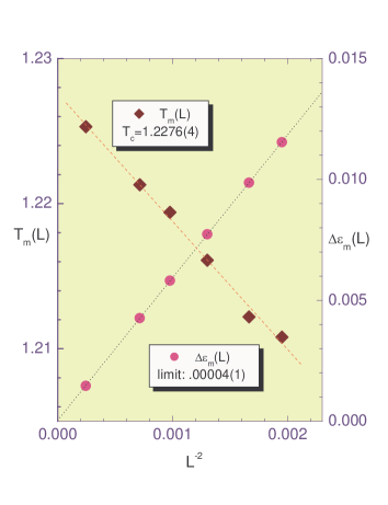
Figure 2: The magnitude of the gap minimum (circles, right y-axis scale) approaches zero as the system size goes to infinity. The sequence of the temperatures corresponding to the gap minima, $T_{m}(L)$ (diamonds, left y-axis scale), can be used to provide an estimate of the critical point $T_{c}$.

where positions and weights are given by the appropriate Gauss-Hermite quadratures routine. Besides the obvious advantage of eliminating the cutoff from the numerical integration, this allows me to identify the largest of the Gauss-Hermite roots, ${\bar{y}}_{N}\approx(2N+1)^{1/2}\equiv L$ with the ”transverse size of the system” and employ finite-size scaling concepts. In this fashion, the singular integral equation is approximated as the $N\to\infty$ limit of the sequence of $N\times N$ matrix equations.

I use ”rescaled” variables, i.e. $y=\rho{\bar{y}}$, $\rho=(2RT)^{1/2}$, and divide both sides of (2) by $\rho\sqrt{\pi}$. This transforms (2) to the matrix form

$$\sum_{j=1}^{N}D_{ij}A_{j}^{\nu}=e^{-\epsilon_{\nu}/T}A_{i}^{\nu}$$ (5)

where

$$D_{ij}=\left(\frac{w_{i}w_{j}}{\pi}\right)^{1/2}e^{{\bar{y}}^{i}{\bar{y}}^{j}}e^{-({\bar{y}}^{i}-{\bar{y}}^{j})^{2}/2}G(\rho{\bar{y}}^{i},\rho{\bar{y}}^{j})$$ (6)

and $\Lambda_{\nu}/(2\pi RT)^{1/2}\equiv e^{-\epsilon_{\nu}/T}$. The advantage of the latter rescaling is that the ”harmonic background” of the free energy has now been absorbed in the prefactor; the lowest of the $\epsilon_{\nu}$ ’s expresses the nontrivial part of the free energy.

I have solved numerically numerics the matrix eigenvalue problem (5) for $R=10.1$ DTP $,N=256,384,512,2048$ and temperatures in the range $0.85<T<1.30$. Results for the difference between the two lowest eigenvalues are shown in Fig. 1. At any given size $L$, the gap has a minimum $\Delta\epsilon_{m}(L)$ at a certain temperature $T_{m}(L)$. Fig. 2 demonstrates that (i) the value of the gap approaches zero quadratically as $L\to\infty$ to within $10^{-5}$ and (ii) the sequence of $T_{m}(L)$’s also approaches a limiting value $T_{c}=1.2276$ quadratically.

I identify the limiting temperature $T_{c}$, where the spectral gap of the limiting, infinite-dimensional matrix eigenvalue equation (5) vanishes, as the transition temperature of the original TI equation (2).

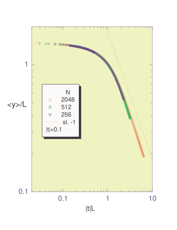
Figure 3: Finite-size scaling of the order parameter. The scaling variable reflects the choice $\nu_{\perp}=1$. Data from the neighborhood of $T_{c}$ (i.e. $|t|<0.1$ for different values of $N$ tend to fall on the same curve; this confirms the choice of $\nu_{\perp}$; the asymptotic slope (dotted line) reflects the property $\nu_{\perp}=-\beta=1$ (cf. text).

Near the critical temperature $T_{c}$, the various thermal properties of a finite-size system exhibit the competition of two transverse length scales: the size of the system $L$ (here: $L=(2N+1)^{1/2}$) and the transverse correlation length $\xi_{\perp}=\left[\left<(\delta y)^{2}\right>\right]^{1/2}\equiv\left[\left<y^{2}\right>-\left<y\right>^{2}\right]^{1/2}$. If (2) has the same critical properties as the Schrödinger-like equation derived from it within the gradient-expansion approximation (e.g. DTP ), we expect, in the limit of infinite $L$, a transverse correlation length $\xi_{\perp}\propto\left|t\right|^{-\nu_{\perp}}$ and an order parameter (OP) $\left<y\right>\propto\left|t\right|^{\beta}$ with $\beta=-\nu_{\perp}=-1$ and $t=T/T_{c}-1$. Then the order parameter in the finite system scales as

$$\left<y\right>_{L}=Lf_{1}\left(\frac{L}{\xi_{\perp}}\right)$$ (7)

where $f_{1}(0)=const$, and $f_{1}(x)\propto 1/x$ if $x>>1$; the first property follows from the requirement of bounded, nonzero OP at $t=0^{-}$ and finite $L$, and the second from the requirement of an $L$-independent limit at values $L>>\xi_{\perp}$; the second property guarantees that $\beta=-\nu_{\perp}$, as expected. Fig. 3 shows that numerical results obtained for three different values of $N$ scale properly if $\nu_{\perp}$ is chosen to be equal to unity.

Similarly, the OP fluctuations scale according to

$$\left<(\delta y)^{2}\right>_{L}^{1/2}=Lf_{2}\left(\frac{L}{\xi_{\perp}}\right)$$ (8)

where now $f_{2}(0)=const$, $f_{2}(x)\propto 1/x$ if $x>>1$ (cf. above, following Eq, 7).

As a consequence of Eqs. (7) and (8), the ratio

$$\frac{\left<(\delta y)^{2}\right>_{L}^{1/2}}{\left<\delta y\right>_{L}}=const.$$ (9)

at $t=0$ and any $L$. This provides a convenient graphical rule for locating the critical point (cf. Fig. 4 and Ref. CuleHwa ). The rule is valid as long as $\beta=-\nu_{\perp}$, i.e. for both 2nd and 1st order instabilities - in the latter case of course only those with a continuously divergent OP .

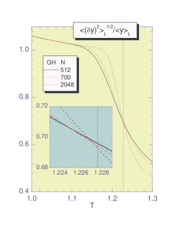
Figure 4: “Reduced” fluctuations of the order parameter for three different values of $N$. The common intersection provides a further method to estimate $T_{c}$ from finite-$N$ runs. Details of the intersection are shown in the inset, along with the estimate $T_{c}=1.2276$ (dashed line) obtained above (cf. Fig. 2).

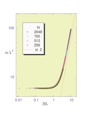
Figure 5: Finite-size scaling of the gap.

The finite-size scaling of the gap is described according to the Ansatz

$$\Delta\epsilon_{L}(t)=L^{-2}f_{G}\left(\frac{L}{\xi_{\perp}}\right)\quad,$$ (10)

where now $f_{G}(0)=const$, $f_{G}(x)\propto x^{2}$ if $x>>1$ (cf. above), and as a result, $\Delta\epsilon_{\infty}(t)\propto|t|^{\nu}$ with $\nu=2$.

Numerical results shown in Fig. 5 demonstrate the validity of the Ansatz (10).

Figure 6: The three lowest eigenvalues of (5) at $T=1.5$ (full symbols) for various $N$. For comparison, the three lowest eigenvalues of (5) with $V=0$ (harmonic chain) are shown (open symbols). The onset shows the same data plotted as $\epsilon_{n}/(n/L)^{2}$ vs. $1/L$; it demonstrates numerically that both sets of eigenvalues behave as $(n/L)^{2}$ at large $L$.

I conclude by presenting some typical results of the spectra of (5) at temperatures above $T_{c}$. Fig. 6 shows the values obtained for $\epsilon_{n}$, $n=1,2,3$, for $T=1.5$ and various $N$. For comparison, I have also plotted the corresponding results obtained in the absence of the Morse potential (harmonic crystal); note that the system size in this case is twice as large, since there is no repulsive barrier at negative $y$. The figure demonstrates that in the limit of large $L$ the spectra of both systems behave as $\epsilon_{n}\propto(n/L)^{2}$. In other words, a detailed analysis of the spectra of (5) can be used to demonstrate that the thermodynamic properties of the high temperature phase coincide exactly with those of the harmonic chain. This completes the thermodynamic description of the instability of the paricle lattice system as the transition from a confined to a deconfined state.

In summary, I have demonstrated that it is possible to view the singular TI thermodynamics of one-dimensional lattice systems with a nearest-neighbor harmonic coupling and a Morse on-site potential as the limit of a sequence of finite matrix eigenvalue problems. The finite-size scaling properties of the sequence are consistent with the universality hypothesis; in other words, the critical exponents of the limiting system with $R=10.1$ are all identical with those obtained via the gradient expansion and the resulting Schrödinger-like equation (under the condition $R<<1$). The procedure described - and, in particular the vanishing of the gap in the limit of infinite system size - constitutes in effect a ”proof” that a phase transition occurs within the framework of the exact TI thermodynamics.

I thank M. Peyrard, T. Dauxois and J. Jäckle for helpful discussions and comments.

References

- (1) L. D. Landau and E. M. Lifshitz, Statistical Physics, Pergamon Press (1980).
- (2) S.K. Sarker and A. Krumhansl, Phys. Rev. B23, 2374 (1981).
- (3) D. M. Kroll and R. Lipowski, Phys. Rev. B28, 5273 (1983); R. Lipowski, Phys. Rev. B32, 1731 (1985).
- (4) M. Peyrard and A.R. Bishop, Phys. Rev. Lett. 62, 2755 (1989).
- (5) T. Dauxois, N. Theodorakopoulos and M. Peyrard, J. Stat. Phys. 107, 869 (2002).
- (6) The essential features of the Morse potential are its repulsive core, stable minimum and flat top. The issue discussed in this note is therefore relevant to related potentials with similar properties (e.g. Lennard-Jones).
- (7) G. Parisi, Statistical Field Theory, Perseus (1998), page 221.
- (8) L. van Hove, Physica 16, 137 (1950).
- (9) F. Gursey, Proc. Cambridge Phil. Soc. 46, 182 (1950).
- (10) D. Ruelle, Commun. Math. Phys. 9, 267 (1968)
- (11) Y-L Zhang, W-M Zheng, J-X Liu, Y. Z. Chen, Phys. Rev. E56, 7100 (1997).
- (12) D.B. Abraham and E.R. Smith, Phys. Rev. B26, 1480 (1982), in the context of surface-film thickening, treat such a case of a singular integral equation, which however arises from an additive on-site term in the left-hand of (2), rather than a proper on-site potential.
- (13) R. A. Guyer and M. D. Miller, Phys. Rev. A17, 1205 (1978).
- (14) T. Dauxois and M. Peyrard, Phys. Rev. E51, 4027 (1995).
- (15) The odds are against the skeptic. In accordance with the universality hypothesis, the Schrödinger equation scenario (gradual disappearance of the bound state in an asymmetric potential) survives in the presence of “perturbations” perhaps more radical than the transition from to : systems with spin-like, integer degrees of freedom, which have been proposed in the context of roughening theories, exhibit exactly the same type of second-order transition as in Refs KroLip or PB -DTP , as long as the on-site potential includes a repulsive core and a short-range attractive part [cf. S.T. Chui and J.D. Weeks, Phys. Rev. B23, 2438 (1981), J.M.J. van Leeuwen and H.J. Hilhorst, Physica 107A, 319 (1981)].
- (16) The matrix eigenvalue problem was solved with the IMSL devesf subroutine. The roots and weights of Gauss - Hermite quadratures with were computed with the zehega and wehega subroutines (double precision) of the splib package developed by D. Funaro (University of Pavia), available at ftp.ian.pv.cnr.it/pub/splib/ . The roots and weights for , computed to quadruple accuracy, were supplied by M. Peyrard (personal communication).
- (17) D. Cule and T. Hwa, Phys. Rev. Lett. 79, 2375 (1997).