Arrays of Cooper Pair Boxes Coupled to a Superconducting Reservoir:
‘Superradiance’ and ‘Revival.’

Abstract

We consider an array of $l_{b}$ Cooper Pair Boxes, each of which is coupled to a superconducting reservoir by a capacitive tunnel junction. We discuss two effects that probe not just the quantum nature of the islands, but also of the superconducting reservoir coupled to them. These are analogues to the well-known quantum optical effects ‘superradiance,’ and ‘revival.’ When revival is extended to multiple systems, we find that ‘entanglement revival’ can also be observed. In order to study the above effects, we utilise a highly simplified model for these systems in which all the single-electron energy eigenvalues are set to be the same (the strong coupling limit), as are the charging energies of the Cooper Pair Boxes, allowing the whole system to be represented by two coupled quantum spins, one finite, which represents the array of boxes, and one representing the reservoir, which we consider in the limit of infinite size. Although this simplification is drastic, the model retains the main features necessary to capture the phenomena of interest. Given the progress in superconducting box experiments over recent years, it is possible that experiments to investigate both of these interesting quantum coherent phenomena could be performed in the forseeable future.

1 Introduction

Recently there has been much interest, both theoretical [1, 2] and experimental [3, 4, 5, 6], in superconducting islands coupled to superconducting reservoirs through Josephson tunnel barriers. Such structures can be manufactured with energy levels such that the islands approximate two - level systems, and may have applications as qubits [7]. In particular, work has focussed on demonstrating the quantum mechanical nature of these systems relevant to quantum computing. A full demonstration of many-qubit quantum algorithms in these systems may be difficult at present, and it may be helpful to find more general indicators of the quantum coherent nature of these systems without the need to, for example, measure a Bell inequality. An ability to demonstrate coherence is a prerequisite for any quantum computer, and so could function as a helpful first step. In particular, revival demonstrates coherence on a timescale which is long compared to the simple oscillation period. This demonstrates that the decoherence time is long enough for multiple gate operations to be performed.

In this paper, we discuss two effects that probe not just the quantum nature of the islands, but also of the superconducting reservoir coupled to them. The first is an analogue to superradiance in quantum optics [8], in which the intensity of the radiation emitted from a collection of atoms is proportional to the square of the number of atoms rather than linearly proportional. Arrays of Josephson junctions coupled through a cavity [9] have also demonstrated enhanced emission of radiation (Barbara et al[10]). Here we consider the current emitted from an array of Cooper Pair Boxes coupled through a superconducting reservoir, which we call the super-Josephson effect.

The second effect is the phenomenon known in quantum optics as revival. In this, the coherent superposition properties of an initial quantum state decay through coupling to the quantum degrees of freedom of the reservoir, and then ‘revive’ at a later time.

When revival is extended to two or more two-level systems we discovered a new phenomenon: ‘entanglement revival.’

In order to study the above effects, we utilise a highly simplified model for the corresponding systems of superconductors. Although the principle simplification, which is to set all the single-electron energy eigenvalues to be the same, is drastic, the model retains the main physical features necessary to capture the phenomena of interest. For example, the essential feature needed to observe revival is the discreteness of the Cooper Pairs in the small superconductors and the reservoir.

2 The Model

2.1 Motivation

The Josephson effect is an intrinsically quantum mechanical phenomenon, as is superconductivity itself. However, in the BCS approximation for a bulk superconductor the phase of the order parameter is usually treated as a classical variable [11], in the sense that fluctuations about it are considered negligible. When the size of the superconductor is reduced, these fluctuations become relevant, and the mean-field treatment is no longer valid. Such deviations from mean field have been observed in experiments on superconducting nanoparticles by Ralph, Black and Tinkham (RBT) [12]. Subsequent work in the field is well reviewed in [13].

In what follows we shall be concerned with the same fluctuations about the mean field theory, albeit for slightly larger superconducting samples, $\sim 100nm$, than in the RBT experiment [12].

In general, to go beyond the BCS approximation is quite difficult even for a single bulk superconductor. Although an exact solution exists for a finite size sample [14, 15], this returns a set of coupled equations which rapidly becomes intractable for a superconductor with more than a few levels.

In our case the difficulty will be compounded by the fact that we wish to treat an array of small superconductors individually coupled to a large one. Thus, to render the problem tractable we shall introduce a highly simplified description of each component of our system. Nevertheless, we shall endeavour to retain sufficient realism to capture some generic features of a number of surprising novel phenomena. These arise when we study the collective quantum states of an array of small superconductors which are not coupled to each other but individually coupled to a common large superconductor; a Cooper Pair reservoir. The model will be introduced in subsections 2.2 and 2.3. The two new phenomena whose description is the principle aim of this paper, namely the superconducting analogues of the quantum optical phenomena of ‘superradiance’ and ‘revival,’ will be treated in sections 3 and 4 respectively.

2.2 The Cooper Pair Boxes

Figure 1: An array of $l_{b}$ superconducting islands, or Cooper Pair Boxes, that are individually coupled to a superconducting reservoir, $r$, through capacitive Josephson tunnel junctions (with no inter-box coupling).

The system we shall study is depicted, schematically, in Figure 1. It consists of an uncoupled array of small superconductors, which we shall refer to as Cooper Pair Boxes, each of which is coupled through tunnel junctions to the same bulk superconductor which we shall call the reservoir. The number of Cooper Pair Boxes will be denoted by $l_{b}$.

The hamiltonian of the system is:

$$H=H_{b}+H_{r}+H_{T}$$ (1)

where the individual hamiltonians refer to the array of Cooper Pair boxes, the reservoir, and the tunneling between the two respectively. The first term is the hamiltonian of the boxes:

$$H_{b}=\sum\limits_{i=0}^{l_{b}}{E_{i}^{ch}\sigma^{z}_{i}}$$ (2)

Each Cooper Pair Box is capacitively gated in such a way that it can be described as a two-level system where the two states are zero or one excess Cooper Pair on the box, with $E_{i}^{ch}$ the charging energy of each. In short, they are the objects investigated in the experiments of Nakamura et. al. [3, 5].

The second term $H_{r}$ is the well known BCS hamiltonian [11] (see section 2.3), and the final term:

$$H_{T}=-\sum\limits_{k,i}{T_{i,k}\;(\sigma_{i}^{+}c_{-k\downarrow}c_{k\uparrow}+\sigma_{i}^{-}c_{k\uparrow}^{\dagger}c_{-k\downarrow}^{\dagger})}$$ (3)

describes the tunnelling of Cooper Pairs from each of the boxes to the reservoir (this form can be derived from single-electron tunnelling [16] with $T_{i,k}$ proportional to the square of the single electron tunnelling energy, $t_{i,k}^{2}$). The charging energy of each box can effectively be tuned by applying a gate voltage to that box, and a tuneable tunnelling energy can be achieved by adjusting the flux through a system of two tunnel junctions in parallel [2]. If the charging energies $E_{i}^{ch}$ and tunnelling elements $T_{i,k}$ of each box are all adjusted to be the same, then the charging energy for all the boxes acts like the z-component of a quantum spin with $J=l_{b}/2$. Similarly the sum over all the raising (lowering) operators acts like a large-spin raising (lowering) operator.

$$\sum\limits_{i=0}^{l_{b}}\sigma_{i}^{Z} \rightarrow S^{Z}_{b}$$

$$\sum\limits_{i=0}^{l_{b}}\sigma_{i}^{\pm} \rightarrow S^{\pm}_{b}$$ (4)

If we consider transitions between the states of the whole system of boxes caused by only these operators, then the symmetrised number states form a complete set. The eigenstates of $S^{Z}_{b}$ represent states where a given number of the boxes are occupied, with $m=N_{b}-l_{b}/2$. We now have a description of the Cooper-Pair boxes in terms of a single quantum spin:

$$H_{b} = E^{ch}_{b}S^{Z}_{b}$$

$$H_{T} = \sum\limits_{k}-T_{k}(S^{+}_{b}c_{-k\downarrow}c_{k\uparrow}+S^{-}_{b}c_{k\uparrow}^{\dagger}c_{-k\downarrow}^{\dagger})$$ (5)

2.3 The Cooper Pair Reservoir

The quantum properties of the reservoir will also be of interest and hence we must simplify its description as well. To do this we start with the BCS Hamiltonian written in terms of the Nambu spins [17], $(\sigma^{Z}_{k}=\frac{1}{2}(c^{{\dagger}}_{k\uparrow}c_{k\uparrow}+c^{{\dagger}}_{-k\downarrow}c_{-k\downarrow}-1),\;\sigma^{+}_{k}=c^{{\dagger}}_{k\uparrow}c^{{\dagger}}_{-k\downarrow})$:

$$H_{r} = \sum\limits_{k}{2(\epsilon_{k}-\mu)\sigma_{k}^{Z}}-\sum\limits_{k=k_{F}-\omega_{c}}^{k_{F}+\omega_{c}}{(\sigma_{k}^{+}\Delta+\sigma_{k}^{-}\Delta^{*})}$$

where $k$ is a generic label (not necessarily the wavevector) of the single-electron eigenstates and the pairing field, for an electron-electron coupling constant $V$, is given by $\Delta_{k}=V\langle\sigma_{k}^{-}\rangle=V\langle c_{-k\downarrow}c_{k\uparrow}\rangle$. As usual, this has to be determined self-consistently.

We shall now make the approximation that the pairing fields, $\Delta_{k},\Delta_{k}^{*}$, are independent of $k$, and that the term $2(\epsilon_{k}-\mu)$ is also the same for all $k$. Remembering that the interaction only occurs in a small region around the Fermi energy, $\epsilon_{F}\pm\omega_{c}$, the approximation that all the $\epsilon_{k}$ are equal is equivalent to taking the limit $\omega_{c}\ll V$ (see A). Clearly this is a drastic, strong coupling, approximation [18, 19, 20], but we will demonstrate that it nevertheless retains some important features of the superconducting state. The gain in making this approximation is that now the Nambu spins can be treated as a single large spin. Further discussion of the justification of this model when the superconductor is finite and its relation to the Richardson solution can be found in [19]. Note however, that Yuzbashyan et. al. [19] are concerned only with isolated islands with a constant number of Cooper Pairs and therefore discard the diagonal term $S^{Z}_{r}$ ($K^{Z}$).

This representation of a sum over Nambu spins as a single spin was used by Lee and Scully in 1971 [21], but that paper discarded the commutator $[S^{+}_{r,\hat{n}},S^{-}_{r,\hat{n}}]=2S^{Z}_{r,\hat{n}}$. By retaining it, we can deal with the discreteness of the Cooper Pairs. The size of the spin is given by $S_{r}=l_{r}/2$ where $l_{r}$ is the number of levels within the cutoff region, which is proportional to the volume and will be taken to infinity at the end of the calculation.

In the above limit the hamiltonian (2.3) becomes:

$$H_{r} = 2\xi_{Fr}S^{Z}_{r}-S^{+}_{r}\Delta-S_{r}^{-}\Delta^{*}$$

Where $(\epsilon_{Fr}-\mu)$ is written as $\xi_{Fr}$ for convenience.

Before treating the coupled system of boxes plus reservoir, we investigate the behaviour of the reservoir alone, in order to demonstrate that our description still makes sense even after the above approximation.

The hamiltonian of the reservoir (2.3) is composed of the $S^{Z}_{r}$, $S^{+}_{r}$ and $S^{-}_{r}$ operators, and so can be written as the component of spin along some other direction $\hat{n}$.

Thus we attempt to diagonalise $H_{r}$ by defining $S^{Z}_{r,\hat{n}}$ by $\gamma_{r}S^{Z}_{r,\hat{n}}=H_{r}$. Then the commutation relations $[S^{Z}_{r,\hat{n}},S^{+}_{r,\hat{n}}]=S^{+}_{r,\hat{n}}$ and $[S^{+}_{r,\hat{n}},S^{-}_{r,\hat{n}}]=2S^{Z}_{r,\hat{n}}$ lead us to the raising and lowering operators in this direction:

$$\gamma_{r}S^{Z}_{r,\hat{n}} = 2\xi_{Fr}S^{Z}_{r}-S^{+}_{r}\Delta-S_{r}^{-}\Delta^{*}$$

$$S^{+}_{r,\hat{n}} = dS^{Z}_{r}+eS^{+}_{r}+fS^{-}_{r}$$

$$|d| = |\Delta|/E_{F}$$

$$e = \frac{-d\Delta}{2\xi_{Fr}-2E_{F}}$$

$$f = \frac{-d\Delta^{*}}{2\xi_{Fr}+2E_{F}}$$

Where $\gamma_{r}=E_{F}=\sqrt{\xi_{Fr}^{2}+|\Delta|^{2}}$, i.e. the quasiparticle energy evaluated at the Fermi energy.

The ground state of the hamiltonian is, obviously, the $m=-l_{r}/2$ eigenstate in the new basis. In the old basis, this is the spin coherent state [22]:

$$|\alpha\rangle = \frac{1}{\sqrt{1+|\alpha|^{2}}}\sum\limits_{N_{r}=0}^{l_{r}}\frac{(\alpha^{*}S_{r}^{+})^{N}_{r}}{N_{r}!}|0\rangle$$ (9)

which can be rewritten as:

$$|\alpha\rangle = \frac{1}{\sqrt{1+|\alpha|^{2}}}\prod\limits_{k}{(1+\alpha^{*}\sigma^{+}_{k})}|0\rangle$$ (10)

As can be readily ascertained using $S_{r,\hat{n}}^{Z}|\alpha\rangle=-l_{r}/2\;|\alpha\rangle$, choosing $\alpha=\frac{\xi_{Fr}-E_{F}}{\Delta}$ ensures that this is the ground state.

In the second expression for $|\alpha\rangle$ we have explicitly rewritten the coherent state as a product over $k$. In this form it is clear that this state is identical to the BCS state in the limit $\omega_{c}\ll V$, when $u_{k}=v_{k}=1\sqrt{2}$. The pairing parameter $\Delta$ and the chemical potential $\mu$ are determined self consistently. In the conventional BCS theory [11]:

$$\frac{\Delta}{V} = \frac{1}{2}\sum\limits_{k}\frac{\Delta}{E_{k}}$$

$$\bar{N}_{r} = \frac{1}{2}\sum\limits_{k}\left(1-\frac{\xi_{k}}{E_{k}}\right)$$ (11)

For our simplified spin model, the fact that the $\epsilon_{k}$ are equal allows us to evaluate the sums in (2.3), giving two coupled algebraic relations instead of integral equations. Thus we can evaluate $\Delta$ and $\mu$ exactly. We find:

$$|\Delta|^{2} = V^{2}\bar{N}_{r}(l_{r}-\bar{N}_{r})$$ (12)

$$\epsilon_{Fr}-\mu = V(l_{r}/2-\bar{N}_{r})$$ (13)

In order to check the validity of these relations, we solve the gap equations for a general BCS case, and then take the limit where all the levels have the same energy. To take this limit, we consider a top-hat density of states centred around $\epsilon_{F}$ with width $w$ and height $l/w$. This allows the limit where the bandwidth $w\rightarrow 0$ to be taken whilst keeping a constant number of levels, $l$. As shown in A, at zero temperature the integrals can be calculated exactly. We find:

$$\Delta^{2} = (\xi_{Fr})^{2}\left(\frac{(x+1)^{2}}{(x-1)^{2}}-1\right)+\left(\frac{w}{2}\right)^{2}\left(\frac{(x-1)^{2}}{(x+1)^{2}}-1\right)$$ (14)

$$\bar{N}_{r} = \frac{l_{r}}{w}\left(\frac{w}{2}-\sqrt{(\xi_{Fr}+\frac{w}{2})^{2}+\Delta^{2}}+\sqrt{(\xi_{Fr}-\frac{w}{2})^{2}+\Delta^{2}}\right)$$ (15)

With $x=e^{\frac{2w}{Vl_{r}}}$ and $n=\frac{\bar{N}_{r}}{l_{r}}$. These two equations can be solved to give $\Delta$ and $\xi_{Fr}$. When the limit $V/w\rightarrow\infty$ (the strong coupling limit) is taken, we find that we obtain the same results as given by the spin model, (12, 13).

Evidently, the fact that this spin representation reproduces the BCS results, albeit only in the strong coupling limit, lends credibility to our simplified model and allows us to consider the situation we wish to describe, namely that of a series of Cooper Pair Boxes coupled individually to a single superconducting reservoir. The problem is then that of two quantum spins, one finite, which represents the array of Cooper Pair Boxes (labelled $b$) and one for the reservoir (labelled $r$) which will consider in the limit $l_{r}\rightarrow\infty$ at the end of the calculation. In short, we shall consider the hamiltonian:

$$\widehat{H} = E^{ch}_{b}S^{Z}_{b}$$ (16)

$$+ 2\xi_{Fr}S^{Z}_{r}-S^{+}_{r}\Delta-S_{r}^{-}\Delta^{*}$$

$$- T(S^{+}_{b}S^{-}_{r}+S^{+}_{r}S^{-}_{b})$$

3 The Super - Josephson Effect

The first effect we consider is an analogy of superradiance (see e.g. [8]). In quantum optics, this refers to the fact that $l_{b}$ atoms, placed in a particular state and coupled to a mode of the electromagnetic field will emit radiation proportional to the square of the number of atoms. The initial state is one of the form:

$$|\psi(0)\rangle=\left\{|000..111..\rangle+|001..110..\rangle+\cdots+|111..000\rangle\right\}$$ (17)

where $0$ and $1$ indicate that an atom (identified by the place of these numbers in the array which specifies the state $|n_{1},n_{2},n_{3}\dots\rangle$) is in its ground or excited state. Clearly, this state is an eigenstate of the operator for the total number of excited states ($S^{Z}_{b}$), but not of the individual $\sigma^{Z}_{i}$ operators. Note that it is the symmetrised state with a total number of excited states $N_{b}$. Evidently, these are exactly the states described by the model in section 2.2. It is also interesting from the quantum information theoretic point of view that these are highly entangled states. These states could, in principle, be generated by tuneable inter-box coupling [2]. For a carefull discussion of superradiance the reader is referred to the very readable account of Eberly [23]. Note also that Josephson junction arrays placed electromagnetic cavities can emit radiation with similar $l_{b}^{2}$ dependence [10].

In this paper, rather than electromagnetic radiation emitted from atoms (or Josephson junctions) coupled through a cavity, we consider the current that is emitted from an array of Cooper Pair Boxes coupled through a common superconducting reservoir. We consider three cases. The first is when the system is in an eigenstate of both the number operator of the large superconductor, and the operator measuring the total number of Cooper Pairs on the boxes. In this case, whilst our model incorporates the fact that the electrons are paired, there is no phase coherence between these pairs.

This is an artificial case if we think of the boxes coupled to a bulk superconductor, but instead would represent many boxes coupled to an island with only a few levels. If both the box and the reservoir are finite then, of course, the order parameter $|\Delta|$ is zero. The square of the order parameter $|\Delta|^{2}$, however, is non-zero, indicating the presence of pairing between the electrons. It is, however, the closest to superradiance, where the atoms are in a symmetrised number eigenstate, and the field contains a given number of photons. We discuss it here for illustrative purposes. The second case is when the boxes are in a number eigenstate and the reservoir in a coherent state, and finally we consider when the boxes are in a coherent state as well as the reservoir.

3.1 Superradiant Tunnelling Between Number Eigenstates

The simplest case is when both the boxes and the reservoir are in eigenstates of the number operators $S^{Z}_{b},S^{Z}_{r}$ respectively. The unperturbed hamiltonian is:

$$H=E^{ch}_{b}S^{Z}_{b}+2\xi_{Fr}S^{Z}_{r}$$ (18)

The eigenstates of this hamiltonian are product states of the number states $|N_{r}\rangle$ and $|N_{b}\rangle$. These states are equivalent to the usual quantum spin eigenstates $|J,m\rangle$ with $J=l/2$ and $m=N-l/2$.

This hamiltonian is perturbed by the tunnelling hamiltonian:

$$H_{T}=-T(S^{+}_{b}S^{-}_{r}+S^{-}_{b}S^{+}_{r})$$ (19)

and the current, i.e. the rate of change of charge on the island, is given by the commutator of the number operator with the hamiltonian:

$$\frac{d\hat{N}_{b}}{dt}=\frac{d\hat{S}_{b}^{Z}}{dt} = \frac{1}{i\hbar}[\hat{S}_{b}^{Z},H]$$

$$\hat{I} = T(S^{+}_{b}S^{-}_{r}-S^{-}_{b}S^{+}_{r})$$ (20)

The expectation value of the current operator with the ground state is equal to zero, so we go to time dependent perturbation theory:

$$|\psi(t)\rangle = U(t)|\psi(0)\rangle$$

$$|\psi(t)\rangle = \left(1+\frac{1}{i\hbar}\int\limits_{0}^{t}{e^{-iHt^{\prime}/\hbar}H_{T}}e^{-iHt^{\prime}/\hbar}{\rm d}t^{\prime}+\cdots\right)|\psi(0)\rangle$$ (21)

The expectation value of any operator at a given time is, to first order in $H_{T}$:

$$\langle\psi(t)|\hat{I}|\psi(t)\rangle = \langle\psi(0)|\hat{I}|\psi(0)\rangle$$ (22)

$$+ 2\Re\{\langle\psi(0)|\hat{I}\frac{1}{i\hbar}\int\limits_{0}^{t}{e^{iHt^{\prime}/\hbar}H_{T}e^{-iHt^{\prime}/\hbar}{\rm d}t^{\prime}}|\psi(0)\rangle\}$$

The tunnelling hamiltonian and current contain only raising and lowering operators, and so their action on a number eigenstate produces a simple sum over two other number eigenstates, with a time dependent factor from the exponentials.

The current is:

$$\langle\psi(t)|\hat{I}|\psi(t)\rangle = \frac{-2T^{2}}{(i\hbar)^{2}}\int\limits_{0}^{t}{\cos{\left((E^{ch}_{b}-2\xi_{Fr})\;t^{\prime}/\hbar\right)}{\rm d}t^{\prime}}$$

$$\times \left(\langle N_{b}|S^{+}_{b}S^{-}_{b}|N_{b}\rangle\langle N_{r}|S^{-}_{r}S^{+}_{r}|N_{r}\rangle-\langle N_{b}|S^{-}_{b}S^{+}_{b}|N_{b}\rangle\langle N_{r}|S^{+}_{r}S^{-}_{r}|N_{r}\rangle\right)$$

The time dependence is determined by the energy difference between adjacent number eigenstates, i.e. by $E^{ch}_{b}$ and $2\xi_{Fr}$. If we evaluate the expectation values, we find terms like $N_{b}(l_{b}-N_{b})(l_{r}-2N_{r})$ which is quadratic in $l_{b}$ and linear in $l_{r}$ (and vice versa, i.e. terms quadratic in $l_{r}$ and linear in $l_{b}$). In particular, to have the largest effect, we set $N_{b}=l_{b}/2$ i.e. half the boxes are occupied.

$$\langle\psi(t)|\hat{I}|\psi(t)\rangle = \frac{-2T^{2}}{(i\hbar)^{2}}\frac{\sin{\left((E^{ch}_{b}-2\xi_{Fr})t/\hbar\right)}}{\left((E^{ch}_{b}-2\xi_{Fr})/\hbar\right)}\left(\frac{l_{b}}{2}(\frac{l_{b}}{2}+1)(l_{r}-2N_{r})\right)$$

We see that the current is proportional to $l_{b}^{2}$, the square of the number of Cooper Pair boxes. This is in contrast to the situation where the initial state of the boxes is a product state of $l_{b}$ independent wavefunctions, in which any current can be at most linear in the number of boxes. The current is also proportional to $(n_{r}-1/2)l_{r}$, where $n_{r}=N_{r}/l_{r}$, i.e. how far away the large superconductor is from half filling.

3.2 Superradiant Tunnelling Between a Number Eigenstate and a Coherent State

The second case we consider is when the Cooper Pair boxes are in an eigenstate of the number operator, and the large superconductor is in a coherent, that is to say BCS-like, state. We ensure the coherent state of the large superconductor by introducing a pairing parameter into the unperturbed hamiltonian:

$$H=E^{ch}_{b}S^{Z}_{b}+2\xi_{Fr}S^{Z}_{r}-\Delta_{r}S_{r}^{+}-\Delta^{*}_{r}S_{r}^{-}$$ (25)

The ground state of the large superconductor is a coherent state and $\Delta_{r}=\langle S_{r}^{-}\rangle$ can now be found self-consistently (see section 2.3).

We make a basis transform and write the hamiltonian in terms of this new basis, $\hat{n}$:

$$H=E^{ch}_{b}S^{Z}_{b}+2E_{Fr}S^{Z}_{r,\hat{n}}$$ (26)

This basis transform makes the unperturbed hamiltonian simpler, but at the expense of making the perturbation more complicated in the new basis:

$$H_{T} = -T(S^{+}_{b}S^{-}_{r}+S^{-}_{b}S^{+}_{r})$$ (27)

$$= -TS^{+}_{b}(\frac{2\Delta_{r}}{E_{Fr}}S^{Z}_{r,\hat{n}}+f_{r}^{*}S^{+}_{r,\hat{n}}+e_{r}S^{-}_{r,\hat{n}})$$

$$-TS^{-}_{b}(\frac{2\Delta^{*}_{r}}{E_{Fr}}S^{Z}_{r,\hat{n}}+e_{r}^{*}S^{+}_{r,\hat{n}}+f_{r}S^{-}_{r,\hat{n}})$$

Again, the tunnelling current is zero to first order in T, as the boxes are in a number eigenstate. With this basis transform, we can easily calculate the second-order current. Following the same procedure as before, we get:

$$\langle\psi(t)|\hat{I}|\psi(t)\rangle = \frac{-2T^{2}}{(i\hbar)^{2}}\frac{|\Delta_{r}|^{2}}{E_{Fr}^{2}}\langle 0_{r,\hat{n}}|S^{Z}_{r,\hat{n}}S^{Z}_{r,\hat{n}}|0_{r,\hat{n}}\rangle\int\limits_{0}^{t}{\rm d}t^{\prime}\cos{E^{ch}_{b}\;t^{\prime}/\hbar}$$ (28)

$$\times(\langle N_{b}|S^{+}_{b}S^{-}_{b}|N_{b}\rangle-\langle N_{b}|S^{-}_{b}S^{+}_{b}|N_{b}\rangle)$$

$$- \frac{2T^{2}}{(i\hbar)^{2}}\langle 0_{r,\hat{n}}|S^{-}_{r,\hat{n}}S^{+}_{r,\hat{n}}|0_{r,\hat{n}}\rangle\times$$

$$\{|e|^{2}\int\limits_{0}^{t}{\rm d}t^{\prime}\left(\cos{(2E_{Fr}-E^{ch}_{b})\;t^{\prime}/\hbar}\right)\langle N_{b}|S^{+}_{b}S^{-}_{b}|N_{b}\rangle$$

$$-|f|^{2}\int\limits_{0}^{t}{\rm d}t^{\prime}\cos{\left((2E_{Fr}+E^{ch}_{b})\;t^{\prime}/\hbar\right)}\langle N_{b}|S^{-}_{b}S^{+}_{b}|N_{b}\rangle\}$$

The time dependence is again given by the level spacing, but for the large superconductor this is now given by $E_{Fr}=\sqrt{\xi_{Fr}^{2}+|\Delta|^{2}}$ rather than $(\epsilon_{Fr}-\mu)$.

If we assume the levels of the large superconductor are much more finely spaced than those of the boxes, i.e. $E_{Fr}\ll E^{ch}_{b}$, then:

$$\langle\psi(t)|\hat{I}|\psi(t)\rangle$$

$$=\frac{-2T^{2}}{(i\hbar)^{2}}\frac{\sin{\left(E^{ch}_{b}t/\hbar\right)}}{E^{ch}_{b}/\hbar}\frac{|\Delta_{r}|^{2}}{E_{Fr}^{2}}\left(\frac{l_{r}}{2}\right)^{2}(l_{b}-2N_{b})$$

$$-\frac{2T^{2}}{(i\hbar)^{2}}\frac{\sin{\left(E^{ch}_{b}t/\hbar\right)}}{E^{ch}_{b}/\hbar}l_{r}\Big{\{}\frac{\xi_{Fr}}{E_{Fr}}N_{b}(l_{b}-N_{b})+|e|^{2}N_{b}-|f|^{2}(l_{b}-N_{b})\Big{\}}$$

Remembering that $l_{r}\xi_{Fr}/E_{Fr}=l_{r}/2-\bar{N}_{r}$, and setting $N_{b}=l_{b}/2$, we find this is proportional to:

$$l_{r}(1-2\bar{n}_{r})\frac{l_{b}}{2}(\frac{l_{b}}{2}+1)$$ (30)

This is very similar to the case described in (3.1) where both the boxes and the reservoir are in number eigenstates. In both cases, the effect is largest when the boxes are at half-filling, and the large superconductor is far from half-filling. The difference is that here it is the average number $\bar{N}_{r}$ that is relevant, not the number eigenvalue.

3.3 Superradiant Tunnelling Between Coherent States

The third case is where both the boxes and the large superconductors are in the coherent state. Pairing parameters are introduced for each:

$$H = 2\xi_{Fb}S^{Z}_{b}-\Delta_{b}S_{b}^{+}-\Delta^{*}_{b}S_{b}^{-}$$ (31)

$$+ 2\xi_{Fr}S^{Z}_{r}-\Delta_{r}S_{r}^{+}-\Delta^{*}_{r}S_{r}^{-}$$

The ground state of this hamiltonian is for both superconductors to be in a coherent state, which again is determined self consistently. As before we make a change of basis, this time for both the boxes and the large superconductor, which makes the unperturbed hamiltonian:

$$H=2E_{Fb}S^{Z}_{b,\hat{n}}+2E_{Fr}S^{Z}_{r,\hat{n}}$$ (32)

The tunnelling hamiltonian becomes:

$$H_{T} = -T(S^{+}_{b}S^{-}_{r}+S^{-}_{b}S^{+}_{r})$$

$$= -T(\frac{\Delta^{*}_{b}}{E_{Fb}}S^{Z}_{b,\hat{n}}+e_{b}^{*}S^{+}_{b,\hat{n}}+f_{b}S^{-}_{b,\hat{n}})(\frac{\Delta_{r}}{E_{Fr}}S^{Z}_{r,\hat{n}}+f_{r}^{*}S^{+}_{r,\hat{n}}+e_{r}S^{-}_{r,\hat{n}})$$

$$-T(\frac{\Delta_{b}}{E_{Fb}}S^{Z}_{b,\hat{n}}+f_{b}^{*}S^{+}_{b,\hat{n}}+e_{b}S^{-}_{b,\hat{n}})(\frac{\Delta^{*}_{r}}{E_{Fr}}S^{Z}_{r,\hat{n}}+e_{r}^{*}S^{+}_{r,\hat{n}}+f_{r}S^{-}_{r,\hat{n}})$$

If we insert this into (22) we find that we do have a non-zero term linear in $T$, i.e. the expectation value of $\hat{I}$ with $|\psi(0)\rangle$. To second order in $T$ we have terms proportional to $l_{r}$ and quadratic in $l_{b}$ and vice versa, and terms linear in both, i.e.

$$\langle\psi(t)|\hat{I}|\psi(t)\rangle = \langle\psi(0)|\hat{I}|\psi(0)\rangle+\langle\psi(t)|\hat{I}|\psi(t)\rangle_{l_{b}^{2}l_{r}}$$ (34)

$$+\langle\psi(t)|\hat{I}|\psi(t)\rangle_{l_{b}l_{r}^{2}}+\langle\psi(t)|\hat{I}|\psi(t)\rangle_{l_{b}l_{r}}$$

The first term is just the expectation value of $\hat{I}$ with the ground state:

$$\langle\psi(0)|\hat{I}|\psi(0)\rangle = \frac{T}{i\hbar}\frac{|\Delta_{b}|}{2E_{Fb}}\frac{|\Delta_{r}|}{2E_{Fr}}\;l_{b}\;l_{r}\;2\sin{(\phi_{b}-\phi_{r})}$$ (35)

$$= \frac{T}{i\hbar}\frac{|\Delta_{b}|}{V_{b}}\frac{|\Delta_{r}|}{V_{r}}\;2\sin{(\phi_{b}-\phi_{r})}$$

where $\phi_{b},\phi_{r}$ are the phases of $\Delta_{b},\Delta_{r}$. This is the usual Josephson effect, as expected between two BCS-like states. To see how the tunnelling is enhanced by superradiance, we examine the addtional terms, i.e. the terms quadratic in $l_{b}$ and $l_{r}$.

The term quadratic in $l_{b}$ is:

$$\langle\psi(t)|\hat{I}|\psi(t)\rangle_{l_{b}^{2}l_{r}}$$ (36)

$$= \frac{-T^{2}}{(i\hbar)^{2}}\;l_{b}^{2}l_{r}\;\frac{\sin{2E_{Fr}t/\hbar}}{2E_{Fr}/\hbar}\frac{|\Delta_{b}|^{2}}{2E_{Fb}^{2}}\;\frac{\xi_{Fr}}{E_{Fr}}$$

$$\frac{-T^{2}}{(i\hbar)^{2}}\;l_{b}^{2}l_{r}\;\frac{\cos{2E_{Fr}t/\hbar}}{2E_{Fr}/\hbar}\frac{|\Delta_{b}|^{2}}{4E_{Fb}^{2}}\frac{|\Delta_{r}|^{2}}{4E_{Fr}^{2}}\;2\sin{2(\phi_{b}-\phi_{r})}$$

The first term is proportional to $|\Delta_{b}|^{2}/E_{Fb}^{2}$ and ${\xi_{Fr}}/{E_{Fr}}$, and so is largest when the boxes are half occupied and the large superconductor is far from half occupied. This term is also phase-independent and is like the effects seen in sections 3.1 and 3.2

The second term is largest when both are half occupied, and also depends on the phase difference of the two pairing parameters with a frequency twice that of the usual Josephson effect. As such, it can be considered a higher harmonic in the Josephson current. The term quadratic in $l_{r}$ is identical apart from an anti-symmetric exchange of the labels, $b,r$.

Finally, the term linear in both contains a phase - independent term that is largest when both the boxes and the reservoir are far from half-filling, and a term that is phase dependent with twice the Josephson frequency that is largest at half filling.

$$\langle\psi(t)|\hat{I}|\psi(t)\rangle_{l_{b}l_{r}}$$

$$= \frac{-T^{2}}{(i\hbar)^{2}}\;l_{b}l_{r}\;\frac{\sin{2(E_{Fb}+E_{Fr})t/\hbar}}{2(E_{Fb}+E_{Fr})/\hbar}\left(\frac{\xi_{Fb}^{2}}{4E_{Fb}^{2}}\;\frac{\xi_{Fr}}{E_{Fr}}-\frac{\xi_{Fr}^{2}}{4E_{Fr}^{2}}\;\frac{\xi_{Fb}}{E_{Fb}}\right)$$

$$+ \frac{T^{2}}{(i\hbar)^{2}}\;l_{b}\;l_{r}\;\ \frac{\cos{2(E_{Fb}+E_{Fr})t/\hbar}}{2(E_{Fb}+E_{Fr})/\hbar}\left(\frac{|\Delta_{b}|^{2}}{4E_{Fb}^{2}}\frac{|\Delta_{r}|^{2}}{4E_{Fr}^{2}}2\sin{2(\phi_{b}-\phi_{r})}\right)$$

In summary we conclude that tunnelling into or out of a Cooper Pair reservoir from a coherent ensemble of Cooper Pair Boxes can lead to a tunnelling current proportional to the square of the number of ‘boxes.’ Interestingly, an observation of such scaling, in turn, could be taken as a demonstration of coherence and entanglement of the the ‘boxes’ as such states are necessary to produce the phenomena.

4 A ‘Superconducting Jaynes-Cummings Model’ and Revival

4.1 The Superconducting Analogue of the Jaynes-Cummings Model

Another well-known quantum optical phenomena is that of quantum revival (see e.g. [8]), which occurs when an atom is coupled to a single mode of the electromagnetic field. The initial state of the atom decays, but reappears at a later time. This apparent decay and subsequent revival occur because the environment of the atom is a discrete quantum field. Here we examine a Josephson system analogue. We consider a hamiltonian (eq. 25) discussed in section 3.2, where the hamiltonian for the box has a number state as a ground state, and the reservoir ground state is a BCS-like state. These are the ground states we would expect for an uncoupled box and reservoir. The tunnelling term $H_{T}$ couples these states.

$$H = E^{ch}_{b}S^{Z}_{b}+2\xi_{Fr}S^{Z}_{r}-\Delta S^{+}_{r}-\Delta^{*}S^{-}_{r}$$

$$H_{T} = -T(S^{+}_{b}S^{-}_{r}+S^{-}_{b}S^{+}_{r})$$ (38)

As in section 3.2, we make a basis transform so that the reservoir is written as a quantum spin in another direction.

$$H = E^{ch}_{b}S^{Z}_{b}+2E_{Fr}S^{Z}_{r,\hat{n}}$$

$$H_{T} = -TS^{+}_{b}(\frac{2\Delta_{r}}{E_{Fr}}S^{Z}_{r,\hat{n}}+f_{r}^{*}S^{+}_{r,\hat{n}}+e_{r}S^{-}_{r,\hat{n}})$$ (39)

$$-TS^{-}_{b}(\frac{2\Delta^{*}_{r}}{E_{Fr}}S^{Z}_{r,\hat{n}}+e_{r}^{*}S^{+}_{r,\hat{n}}+f_{r}S^{-}_{r,\hat{n}})$$

We can write a general state of the system in terms of the number eigenstates:

$$|\psi(t)\rangle=\sum\limits_{N_{r},N_{b}=0}^{l_{r},l_{b}}a_{N_{r},N_{b}}(t)|N_{r}\rangle|N_{b}\rangle$$ (40)

For a single two level system, $l_{b}=1$, but we can also do the calculations for a general number of symmetrised boxes. We can calculate the time evolution of the system using the Schrödinger equations:

$$i\hbar\sum\limits_{N_{r},N_{b}}\frac{d\,a_{N_{r},N_{b}}(t)}{dt}|N_{r}\rangle|N_{b}\rangle$$

$$= \sum\limits_{N_{r},N_{b}}a_{N_{r},N_{b}}(t)\left(E^{ch}_{b}(N_{b}-\frac{l_{b}}{2})+2\xi_{Fr}(N_{r}-\frac{l_{r}}{2})\right)|N_{r}\rangle|N_{b}\rangle$$

$$- \sum\limits_{N_{r},N_{b}}a_{N_{r},N_{b}}(t)\,TS^{+}_{b}(\frac{2\Delta_{r}}{E_{Fr}}S^{Z}_{r,\hat{n}}+f_{r}^{*}S^{+}_{r,\hat{n}}+e_{r}S^{-}_{r,\hat{n}})|N_{r}\rangle|N_{b}\rangle$$

$$- \sum\limits_{N_{r},N_{b}}a_{N_{r},N_{b}}(t)\,TS^{-}_{b}(\frac{2\Delta^{*}_{r}}{E_{Fr}}S^{Z}_{r,\hat{n}}+e_{r}^{*}S^{+}_{r,\hat{n}}+f_{r}S^{-}_{r,\hat{n}})|N_{r}\rangle|N_{b}\rangle$$

More explicitly, we have a set of coupled differential equations for the coefficients $a_{N_{r},N_{b}}(t)$:

$$i\hbar\frac{d\,a_{N_{r},N_{b}}(t)}{dt} = a_{N_{r},N_{b}}(t)\left(E^{ch}_{b}(N_{b}-\frac{l_{b}}{2})+2\xi_{Fr}(N_{r}-\frac{l_{r}}{2})\right)$$

$$- a_{N_{r},N_{b}+1}(t)\,T\sqrt{(N_{b}+1)(l_{b}-N_{b})}\frac{2\Delta^{*}_{r}}{E_{Fr}}(N_{r}-l_{r}/2)$$

$$- a_{N_{r}-1,N_{b}+1}(t)\,T\sqrt{(N_{b}+1)(l_{b}-N_{b})}e_{r}^{*}\sqrt{N_{r}(l_{r}-N_{r}+1)}$$

$$- a_{N_{r}+1,N_{b}+1}(t)\,T\sqrt{(N_{b}+1)(l_{b}-N_{b})}f_{r}\sqrt{(N_{r}+1)(l_{r}-N_{r})}$$

$$- a_{N_{r},N_{b}-1}(t)\,T\sqrt{N_{b}(l_{b}-N_{b}+1)}\frac{2\Delta_{r}}{E_{Fr}}(N_{r}-l_{r}/2)$$

$$- a_{N_{r}-1,N_{b}-1}(t)\,T\sqrt{N_{b}(l_{b}-N_{b}+1)}f_{r}^{*}\sqrt{N_{r}(l_{r}-N_{r}+1)}$$

$$- a_{N_{r}+1,N_{b}-1}(t)\,T\sqrt{N_{b}(l_{b}-N_{b}+1)}e_{r}\sqrt{(N_{r}+1)(l_{r}-N_{r})}$$

These equations are tri-diagonal and can be solved numerically. For now, to stimulate interest, we consider an approximation that allows a simple analytical model.

The $\Delta$ terms in eq. 4.1 mean that the total particle number $N_{r}+N_{b}$ is not conserved. We note that whilst the commutator of the total number operator $[\hat{N}_{r}+\hat{N}_{b},\hat{H}]=\Delta S^{+}_{r}-\Delta^{*}S_{r}^{-}$ is not zero, its expectation value in the coherent state is. With this in mind, we approximate and assume no fluctuations in the total number (although we of course retain fluctuations in $N_{r}-N_{b}$) and discard any terms in eq. 4.1 that change the total number.

With these terms discarded, we have a set of coupled differential equations in which each coefficient $a_{N_{r},N_{b}}(t)$ only couples to $a_{N_{r}-1,N_{b}+1}(t)$ and $a_{N_{r}+1,N_{b}-1}(t)$.

$$i\hbar\frac{d\,a_{N_{r},N_{b}}(t)}{dt} = a_{N_{r},N_{b}}(t)\left(E^{ch}_{b}(N_{b}-\frac{l_{b}}{2})+E_{Fr}(N_{r}-\frac{l_{r}}{2})\right)$$

$$- a_{N_{r}+1,N_{b}-1}(t)\,T\sqrt{N_{b}(l_{b}-N_{b}+1)}\sqrt{(N_{r}+1)(l_{r}-N_{r})}$$

$$- a_{N_{r}-1,N_{b}+1}(t)\,T\sqrt{(N_{b}+1)(l_{b}-N_{b})}\sqrt{N_{r}(l_{r}-N_{r}+1)}$$

These equations can be restated in terms of an eigenvalue problem. Each level $N_{r}$ has a set of eigenvectors for the boxes. If the boxes and the reservoir are initially in a product state, the probability to be in a given value of $N_{b}$ (regardless of $N_{r}$) is:

$$P_{N_{b}}=\sum\limits_{N_{b}=0}^{l_{b}}|a_{N_{r}}(0)|^{2}\left|\sum\limits_{i}\langle N_{b}|\nu_{i,N_{r}}\rangle e^{-iE_{i,N_{r}}t/\hbar}\langle\nu_{i,N_{r}}|\psi_{N_{b}}(0)\rangle\right|^{2}$$ (44)

Where $|\nu_{i,N_{r}}\rangle$ ($E_{i,N_{r}}$) are the eigenvectors (values) of the $N_{b}$-level system associated with the reservoir level $|N_{r}\rangle$, $a_{N_{r}}(0)$ are the initial amplitudes of $|N_{r}\rangle$, and $|\psi_{N_{b}}(0)\rangle$ is the initial state of the boxes.

This may not be exactly solvable in general, but can be solved for few-level systems, $l_{b}$. For example, if we have a single two level system and specify the initial state to be a product state of the box state $|0_{b}\rangle$ with some state $\sum a_{N_{r}}(0)|N_{r}\rangle$ of the reservoir, we have the probabilities that the box and reservoir are in a given state:

$$P_{1,N_{r}-1}(t) = |a_{N_{r}}(0)|^{2}\frac{{T^{\prime}_{N_{r}}}^{2}}{{\Omega_{N_{r}}}^{2}}\sin^{2}(\Omega_{N_{r}}t/\hbar)$$

$$P_{0,N_{r}}(t) = |a_{N_{r}}(0)|^{2}\left(1-P_{1,N_{r}-1}(t)\right)$$ (45)

With $T^{\prime}_{N_{r}}=T\sqrt{N_{r}(l_{r}-N_{r}+1)}$ and $\Omega_{N_{r}}=\sqrt{(E^{ch}_{b}-E_{Fr})^{2}/4+{T^{\prime}}^{2}}$. This is the same result as in quantum optics, except that the photon creation/ annihilation operators give $T^{\prime}_{N_{r}}=T\sqrt{N_{r}}$ .

4.2 Quantum Revival of the Initial State

In quantum optics, the phenomenon of revival is seen when the electromagnetic field is placed in a coherent state (i.e. $|a_{N}|^{2}=\exp(-\bar{N})\bar{N}^{N}/N!$, with the sum over $N$ running to infinity). We place the reservoir in the spin coherent state, i.e.

$$|a_{N_{r}}(0)|^{2}=|\alpha|^{2N_{r}}\frac{l_{r}!}{(l_{r}-N_{r})!N_{r}!}$$ (46)

Where $\alpha$ is determined by the average number $|\alpha|=\sqrt{\bar{N_{r}}/(l_{r}-\bar{N}_{r})}$.

The probability of the box being in the state $|0_{b}\rangle$ at a given time is:

$$P_{0}(t)=\sum\limits_{N_{r}}^{l_{r}}|a_{N_{r}}(0)|^{2}P_{0,N_{r}}(t)$$ (47)

For simplicity we consider the case when $E^{ch}_{b}=E_{Fr}$, i.e. $\Omega_{N_{r}}=T^{\prime}_{N_{r}}$. This is shown in Figure 2, for the values $\bar{N}_{r}=10$, $l_{r}=50$. The initial state dies away, to be revived at a later time.

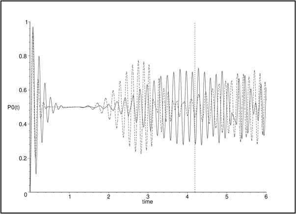
Figure 2: Spin Coherent State Revival for $N_{r}=10$, $l_{r}=50$ (solid line). The faint line indicates the usual quantum optical coherent state revival with $N_{r}=10$, scaled along the $t$ axis by $\sqrt{l_{r}}$ and the vertical dash-dot line indicates the calculated revival time.

The revival occurs when the terms in the sum are in phase. We can make an estimate of this by requiring the terms close to $\bar{N}_{r}$ to be in phase:

$$2\pi = 2T\sqrt{(\bar{N}_{r}+1)(l_{r}-\bar{N}_{r})}\;t_{rev}-2T\sqrt{\bar{N}_{r}(l_{r}-\bar{N}_{r}+1)}\;t_{rev}$$

$$t_{rev} = \frac{2\pi}{T}\frac{\bar{n}_{r}^{1/2}(1-\bar{n}_{r})^{1/2}}{(1-2\bar{n}_{r})}$$ (48)

Where, as before $n_{r}=N_{r}/l_{r}$. Note that the revival time remains finite in the $l_{r}\rightarrow\infty$ limit, as long as $N_{r}/l_{r}$ is finite.

We can find an analytic form for the initial decay, and also demonstrate the equivalence of this ‘spin revival’ to the well known quantum optics revival, in the limit $l_{r}\rightarrow\infty$, $l_{r}/N_{r}\rightarrow\infty$. Note that this is an unrealistic limit for our case, where we would keep the filling factor $N_{r}/l_{r}$ constant, but it allows us to make a connection with the quantum optics case.

Figure 3: The large $\bar{N_{r}},l_{r}$ limit: Solid line indicates single box revival for $N_{r}=10$, $l_{r}=100$, and the dashed line indicates the asymptotic form for the decay.

The coefficients, $a_{N_{r}}(0)$ for the coherent and spin-coherent states are the Poisson and binomial distributions respectively, and both can be approximated by a Gaussian distribution.

$$\exp(-\bar{N}_{r})\bar{N}_{r}^{N_{r}}/N_{r}! \simeq (2\pi\bar{N}_{r})^{-1/2}\exp\left[-(N_{r}-\bar{N}_{r})^{2}/2\bar{N}_{r}\right]$$

$$|\alpha|^{2N_{r}}\frac{l_{r}!}{(l_{r}-N_{r})!N_{r}!} \simeq (2\pi\bar{N}_{r})^{-1/2}\exp\left[-(N_{r}-\bar{N}_{r})^{2}/2\bar{N}_{r}\right]$$ (49)

For the coherent state we have taken the limit $\bar{N}_{r}\gg 1$. For the spin-coherent case we have also assumed $l_{r}\gg\bar{N}_{r}$. The gaussian factor suppresses any terms not around the average $\bar{N}_{r}$, so we can expand $N_{r}\simeq\bar{N}_{r}+(N_{r}-\bar{N}_{r})$.

In the limit, the spin coherent state gives:

$$P_{0}(t) = \frac{1}{2}+\frac{1}{2(2\pi\bar{N})^{1/2}}\int{\rm d}N\,\exp\left(-\frac{(N_{r}-\bar{N}_{r})^{2}}{2\bar{N}_{r}}\right)$$ (50)

$$\times\cos\left[2T({l_{r}\bar{N}_{r}})^{1/2}t\left(1+\frac{(N_{r}-\bar{N}_{r})^{2}}{2\bar{N}_{r}}\right)\right]$$

This is the same as for the coherent state apart from the factor of $l_{r}^{1/2}$ if the frequency. Doing the integral gives:

$$P_{0}(t)=\frac{1}{2}+\frac{1}{2}\cos(2T(l_{r}\bar{N}_{r})^{1/2}t)\;\exp(-\frac{(Tl_{r}t)^{2}}{2})$$ (51)

This is plotted in Figure 3.

Thus the phenomenon of quantum revival has a direct analogy in our ‘spin superconductor’ model. In both cases, the revival is due to constructive interference between the terms in the sum over the reservoir (field) number states.

4.3 Revival of Entanglement

Revival is usually considered for single two-level systems, but the formula in (44) gives the state for a general system. In particular, the dynamics of a pair of two-level systems can be easily calculated, either numerically, or analytically, remembering that the singlet state is uncoupled due to radiation trapping.

Starting in the state $|00\rangle$, we find a very similar effect to the single-island case. When one island is traced out, the revival of the other occurs at the same time as a single island, but with opposite phase (Figure 4).

Figure 4: Two Cooper Pair Box Spin Coherent State Revival for $N_{r}=10$, $l_{r}=50$. The solid line represents the probability that, when the system is initialised in the state $|00\rangle$, one of the Cooper pair boxes is in the state $|0\rangle$ at time $t$, after tracing over the other box. The dashed line indicates the revival of a single isolated Cooper Pair box connected to a reservoir. Note that the revivals occur at the same time, but out of phase.

If we do not trace over one island, but consider the revival of the state $|00\rangle$, we find oscillations in the probability of returning to this state earlier than in the case of a single island.

To investigate the revival of entanglement, we start the system in the state $(|01\rangle+|10\rangle)/\sqrt{2}$. As before we note that the oscillations in the probability of being in the state $(|01\rangle+|10\rangle)/\sqrt{2}$ decay and then revive. It is interesting to note, however, that in this case the initial state is an entangled one. One measure of entanglement is the negativity [24], i.e. the sum of the negative eigenvalues of the partially transposed density matrix. If we plot the negativity over time, we see that it dies away at first, as do the oscillations. As the oscillations revive, we also see an revival in the negativity of the two islands (Figure 5).

Figure 5: Two Cooper Pair Box Spin Coherent State Revival for $N_{r}=10$, $l_{r}=50$. The dashed line represents the probability that the Cooper Pair boxes have returned to their initial state $(|01\rangle+|10\rangle)/\sqrt{2}$ at time $t$. The dashed line indicates the negativity of the boxes as a function of time.

This revival of entanglement, an initially counterintuitive phenomenon, is of course due to the fact that we have considered the entanglement between the two islands only. When the entanglement ‘disappears,’ it is only the entanglement between the islands that has disappeared. If we were to consider the whole system, including the reservoir, the evolution would be unitary and the entanglement would remain constant.

It is worth noting that this ‘entanglement revival’ is not a unique feature of our spin model, and would be expected whenever two-level systems are coupled to a field with (a possibly infinite number of) discrete energy levels.

5 Conclusions

We have presented a simple model of a superconductor that allows an easy investigation of various phenomena associated with fluctuations around the BCS, mean field, behaviour. By taking the limit where all the single-electron energy levels are equal, we can represent the superconducting hamiltonian in terms of the operators of a large, finite quantum spin, which we then consider in the limit $l_{r}\rightarrow\infty$. Comparison of results using this model in the mean field with the limit of BCS results gives us confidence that whilst the model can be regarded as a caricature of a realistic description it retains some generic features of quantum fluctuations. Furthermore, we have demonstrated that the simplicity of the model allows the easy investigation of several surprising physical phenomena.

As the first of these we considered an analogue of the quantum optical effect of superradiance, where the emitted intensity of a number of atoms coupled to an electromagnetic field is proportional to the square of the number of atoms.

In the analogous ‘Super-Josephson effect,’ the current from a set of Cooper Pair boxes connected to a reservoir is proportional to the square of the number of boxes $l_{b}$. This effect is due to the entangled nature of the initial state. Any product state (or mixture of product states) would produce a current at most linear in $l_{b}$. The effect also relies on the reservoir being away from the $N_{r}/l_{r}=1/2$ state, i.e. away from half-filling.

The analogy has been extended to the physically relevant case case where the reservoir is in a coherent (i.e. BCS-like) state and the boxes are in a number state. As before we have no current to first order in $T$, but have a current proportional to $l_{b}^{2}$ to second order. Also as in the previous case, the effect requires the reservoir to be far from half-filling, but here it is the average number $\bar{N}_{r}$ that must be far from $l_{r}/2$.

Finally we considered the effect when both the reservoir and the boxes are initially in a coherent state. In addition to the usual Josephson current, we observe the effect described above and also find a current that is dependent on the phase difference between the superconductors, with twice the phase dependence of the usual Josephson effect.

Interestingly, the above discussion suggests that an observation of a Josephson current which scales quadratically with the number of small superconductors (qubits) can be taken as evidence for their entanglement. As experiments are now at the level of entangling two charge qubits [5], and these effects can be detected by making only current measurements, the above effects could be usefully looked for experimentally.

We have also studied an analogue of quantum revival (again considering the case a box in a number state coupled to a reservoir in a BCS-like state) , in which the oscillations (of the type observed in [3, 4, 5, 6]) in the probability of occupation of an island decay at first, only to revive at a later time. This effect can also be seen when we have two Cooper Pair boxes coupled to a reservoir. If we place these boxes in an entangled state and calculated the entanglement over time, we see that the entanglement between the boxes dies away at first, only to revive later. This remarkable effect demonstrates and measures the quantum fluctuations of the reservoir superconductor about the BCS mean field theory. In other words it probes the discreteness of the Cooper Pairs in the same way as the corresponding quantum optical effect probes the discreteness of photons of the radiation field.

Acknowledgements

We would like to thank James Annett for helpful discussions. Denzil Rodrigues is supported by an EPSRC CASE studentship with sponsorship from Hewlett-Packard.

Appendix A Limit of BCS Self Consistency Equations

As confirmation of the validity of our spin model, we wish to compare it with the standard BCS theory. In particular, we wish to check that solving the gap equations from the spin model gives the same result (12, 13) as if we solve the usual BCS gap equations (2.3) first, and then take the limit. We wish to take the limit where the single-electron energy levels, $\epsilon_{k}$ are equal. To do this we consider a density of states which is a top-hat function centred around $\epsilon_{F}$ with width $\omega$ and height $l_{r}/\omega$. Taking the limit $\omega\rightarrow 0$ ensures that the interaction occurs in a narrow region around $\epsilon_{F}$ whilst ensuring the integral is over a constant number of levels, $l_{r}$. We have two integral equations that must be solved self-consistently. The first is an equation for the pairing parameter, $\Delta$:

$$\frac{\Delta}{V} = \frac{1}{2}\int\limits_{\epsilon_{F}-\omega}^{\epsilon_{F}+\omega}{\rm d}\epsilon\frac{\Delta}{((\epsilon-\mu)^{2}+|\Delta|^{2}))^{\frac{1}{2}}}$$ (52)

and the second is an equation for the average number of Cooper Pairs, $\bar{N}$:

$$\bar{N}=\frac{1}{2}\int\limits_{\epsilon_{F}-\omega}^{\epsilon_{F}+\omega}{\rm d}\epsilon\left(1-\frac{\epsilon-\mu}{((\epsilon-\mu)^{2}+|\Delta|^{2}))^{\frac{1}{2}}}\right)$$ (53)

As we are at zero temperature, both these integrals can be done exactly:

$$\frac{1}{V} = \frac{l}{2\omega}\ln\left(\frac{(\xi_{F}+\omega/2)+\sqrt{(\xi_{F}+\omega/2)^{2}+|\Delta|^{2}}}{(\xi_{F}-\omega/2)+\sqrt{(\xi_{F}-\omega/2)^{2}+|\Delta|^{2}}}\right)$$ (54)

$$\bar{N} = \frac{l}{\omega}\left(\frac{\omega}{2}-\sqrt{(\xi_{F}+\omega/2)^{2}+|\Delta|^{2}}+\sqrt{(\xi_{F}-\omega/2)^{2}+|\Delta|^{2}}\right)$$ (55)

Again, $\xi_{F}$ is shorthand for $\epsilon_{F}-\mu$. These can be rearranged to give two equations for $|\Delta|^{2}$ (56, 57), or two equations for $\xi_{F}^{2}$ (59, 60). The equations for $|\Delta|^{2}$ are:

$$|\Delta|^{2} = (\xi_{F})^{2}\left(\frac{(x+1)^{2}}{(x-1)^{2}}-1\right)+\left(\frac{w}{2}\right)^{2}\left(\frac{(x-1)^{2}}{(x+1)^{2}}-1\right)$$ (56)

$$|\Delta|^{2} = \frac{\bar{N}(l-\bar{N})}{l^{2}(l-2\bar{N})^{2}}\left(4{\xi_{F}}^{2}l^{2}-\omega^{2}(l-2\bar{N})^{2}\right)$$ (57)

Equating the two and rearranging gives us an expression for ${\xi_{F}}^{2}$:

$${\xi_{F}}^{2}=\left(\frac{\omega}{2}\right)^{2}\left(\frac{(x+1)^{2}}{(x-1)^{2}}-1+4(1-2n)^{2}\right)\bigg{/}\left(\frac{4n(1-n)}{(1-2n)^{2}}-\frac{(x-1)^{2}}{(x+1)^{2}}+1\right)$$ (58)

where $x=e^{\frac{2w}{Vl}}$ and $n=\frac{\bar{N}}{l}$. If we rearrange eqns. (54, 55) for $\xi_{F}$ we get:

$${\xi_{F}}^{2} = \left(\frac{\omega}{2}\right)^{2}\frac{(x+1)^{2}}{(x-1)^{2}}-|\Delta|^{2}\frac{(x+1)^{2}}{4x}$$ (59)

$${\xi_{F}}^{2} = \left(\frac{\omega}{2}\right)^{2}(1-2n)^{2}+|\Delta|^{2}\frac{(1-2n)^{2}}{4n(1-n)}$$ (60)

Which yield:

$$|\Delta|^{2}=\left(\frac{\omega}{2}\right)^{2}\left(\frac{(x+1)^{2}}{(x-1)^{2}}-(1-2n)^{2}\right)\bigg{/}\left(\frac{(1-2n)^{2}}{4n(1-n)}+\frac{(x+1)^{2}}{4x}\right)$$ (61)

From eqns. (58, 61), it is clear that the correct limit to take is $\omega/V\rightarrow 0$. Taking this limit of eqns. (58, 61), we get:

$${\xi_{F}}^{2} = \frac{V^{2}l^{2}}{4}(1-2n)^{2}$$ (62)

$$|\Delta|^{2} = V^{2}l^{2}n(1-n)$$ (63)

That is, we have regained the forms for $\Delta$ and $\xi$ given by the spin model (12, 13).

References

References

• [1] Takeo Kato, 2002, J. Low Temp. Phys . 131 25
• [2] Yu. Makhlin, G. Schön A. Shnirman, 2001, Rev. Mod. Phys. 73 357
• [3] Y. Nakamura, Yu. A. Pashkin, J.S. Tsai, 1997, Nature 398, 786
• [4] D. Vion, A. Assime, A. Cottet, P. Joyez, H. Pothier, C. Urbina, D.Esteve, M.H. Devoret, 2002, Science, 296 886
• [5] Yu. A. Pashkin, T. Yamamoto, O. Astafiev, Y. Nakamura, D. V. Averin, J. S. Tsai Nature, 2003, 421, 823
• [6] T. Duty, D. Gunnarsson, K. Bladh, R.J. Schoelkopf, P. Delsing cond-mat/0305433, to appear in Phys. Rev. B
• [7] A. Shnirman, G. Schon, Z. Hermon, 1997, Phys. Rev. Lett. 79, 2371.
• [8] S. Barnett, P. Radmore, Methods in Theoretical Optics, 2, Oxford, 1997
• [9] P. Hadley, M. R. Beasley and K. Weisenfeld, 1988, Phys. Rev. B 38, 8717
• [10] P. Barbara, A. B. Cawthorne, S. V. Shitov and C. J. Lobb, 1999, Phys. Rev. Lett. 82, 1963
• [11] J. Bardeen, L.N. Cooper, J.R. Schriefer, 1957, Phys. Rev. 108 1175
• [12] D.C. Ralph, C.T. Black, M. Tinkham, 1996, Phys. Rev. Lett. 76 688
• [13] Jan von Delft, 2001, Ann. Phys. (Leipzig) 10 1
• [14] R.W. Richardson, 1963, Phys. Rev. Lett. 3, 277
• [15] J. Delft, F. Braun cond-mat/9911058, 2000 NATO ASI Quantum Mesoscopic Phenomena and Mesocscopic Devices in Microelectronics, Eds. I. O. Kulik and R. Elliatioglu, (Dordrecht: Kluwer Ac. Publishers), p. 361
• [16] P.R. Wallace and M.J. Stavn, 1965, Canadian Journal of Physics 43 411
• [17] S. Doniach and E.H. Sondheimer, Green’s functions for solid state physicists Benjamin, 1974.
• [18] J. M. Roman, G. Sierra, J. Dukelsky, 2003, Phys. Rev. B 67, 064510
• [19] E. Yuzbashyan, A. Baytin, B. Altshuler, 2003, Phys. Rev. B 68, 214509
• [20] D.T. Thouless, Quantum mechanics of Many-Body Systems,7 Academic Press, 1972
• [21] Lee and Scully, 1971, Phys. Rev. B. 3 769
• [22] R. Feynman, R. Leyton, M. Sands, Lectures on Physics, Vol. III, 18, Addison-Wesley, 1965
• [23] J. H. Eberly, American Journal of Physics, 40, 1374
• [24] G. Vidal, R.F. Werner, 2002, Phys. Rev. A 65 032314