Fluctuations in network dynamics

Abstract

Most complex networks serve as conduits for various dynamical processes, ranging from mass transfer by chemical reactions in the cell to packet transfer on the Internet. We collected data on the time dependent activity of five natural and technological networks, finding that for each the coupling of the flux fluctuations with the total flux on individual nodes obeys a unique scaling law. We show that the observed scaling can explain the competition between the system’s internal collective dynamics and changes in the external environment, allowing us to predict the relevant scaling exponents.

Recent advances in uncovering the mechanisms shaping the topology of complex networks  networks are overshadowed by our lack of understanding of common organizing principles governing network dynamics. In particular, we are far from understanding how the collective behavior of often millions of nodes contribute to the observable dynamical features of a given system, prompting us to continue the search for dynamical organizing principles that are common to a wide range of complex systems. To make advances in this direction we need to complement the available network maps with data on the time resolved activity of each node and link.

Traditional approaches to complex dynamical systems focus on the long time behavior of at most a few dynamical variables, characterizing either a single node or the system’s average behavior. To simultaneously characterize the dynamics of thousands of nodes we investigate the coupling between the average flux and fluctuations. Our measurements indicate that in complex networks there is a characteristic coupling between the average flux $\left<{f_{i}}\right>$ and dispersion $\sigma_{i}$ of individual nodes (Fig. $1$). To quantify this observation we plot $\sigma_{i}$ for each node $i$ in function of the average flux $\left<{f_{i}}\right>$ of the same node (Figs. 2 & 3). We find that for five systems for which extensive dynamical data is available the dispersion depends on the average flux as

$$\sigma\sim\left<{f}\right>^{\alpha}.$$ (1)

Most intriguing, however, is the finding that the dynamical exponent $\alpha$ is in the vicinity of two distinct values, $\alpha=1/2$ (Fig. 2) and $\alpha=1$ (Fig. 3), suggesting that diverse real systems can display two distinct dynamical universality classes.

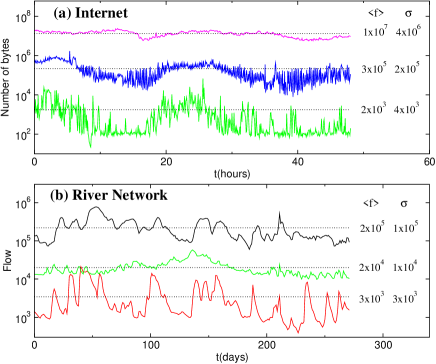
Figure 1: (a) Time dependent traffic on three Internet routers of the Mid-Atlantic Crossroads network, whose activity is monitored by the Multi Router Traffic Grapher software (MRTG). The figure shows the number of bytes per second for each of the routers in five minutes intervals for a two day period. (b) Streamflow, measured in cubic feet per second, on three rivers in the US river basin, based on data collected by the U.S. Geological Survey in $2001$. On the right of each plot we show the time average of the flux $\left<{f}\right>$ displayed as horizontal dotted lines superposed on the graphs, and the dispersion, $\sigma$, for each signal, indicating orders of magnitude differences in both flux and dispersion between nodes of the same network.

The $\alpha\simeq 1/2$ systems (Fig. 2): The Internet, viewed as a network of routers linked by physical connections, serves as a transportation network for information, carried in form of packets  vazquez . Daily traffic measurements of $374$ geographically distinct routers indicate that the relationship between traffic and dispersion follows (1) for close to seven orders of magnitude with $\alpha^{I}=1/2$ (Fig. 2a). In a microprocessor, in which the connections between logic gates generate a static network  sole , information is carried by electric currents. At each clock cycle a certain subset of connections $i$ are active, the relevant dynamical variable $f_{i}(t)$ taking two possible values, $0$ or $1$. The activity during $8,862$ clock cycles on $462$ nodes of the Simple12 microprocessor indicates that the average flux and fluctuations follow (1), with $\alpha^{m}=1/2$ (Fig. 2b).

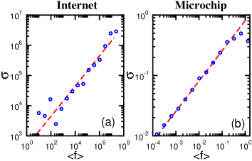
Figure 2: The relationship between fluctuations ($\sigma$) and the average flux ($\left<{f}\right>$) for the $\alpha=1/2$ systems. (a) Time resolved information for $374$ Internet routers of the Mid-Atlantic Crossroads, ABILENE network, MIT routers, UNAM routers, all Brazilian RNP backbones, and dozens of smaller routers on the Internet, covering for each node two days of activity with five minute resolution. (b) The activity of the $462$ signal carriers of the 12-bit Simple12 microprocessor, recorded over $8,862$ clock cycles.

The $\alpha\simeq 1$ systems (Fig. 3): The WWW, an extensive information depository, is a network of documents linked by URLs  lawrence . As many websites record individual visits, surfers collectively contribute to a dynamical variable $f^{w}_{i}(t)$ that represents the number of visits site $i$ receives during day $t$. We studied the daily breakdown of visitation for $30$ days for $3,000$ sites scattered over three continents, determining for each node $i$ the average $\left<{f_{i}^{w}}\right>$ and dispersion $\sigma_{i}^{w}$. As Fig. 3a shows, $\sigma_{i}^{w}$ and $\left<{f_{i}^{w}}\right>$ follow (1) over three orders of magnitude with dynamical exponent $\alpha^{w}=1$. The highway system is an example of a transportation network, the relevant dynamical variable being the traffic at different locations. We analyzed the daily breakdown of traffic measurements at $127$ locations on Colorado and Vermont highways. The results, shown in Fig. 3b, again document scaling spanning over five orders of magnitude with $\alpha^{h}=1$. Finally, the river network is a natural transportation system  banavar , whose dynamics is probed via time resolved measurements on the stream of several US rivers on $3,495$ different locations. While these fluctuations are driven by weather patterns, the relationship between the average stream and its fluctuations again follows (1) with $\alpha^{r}=1$ (Fig. 3c).

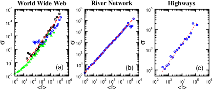
Figure 3: The relationship between fluctuations ($\sigma$) and the average flux ($\left<{f}\right>$) for systems belonging to the $\alpha=1$ class. (a) Daily visitations on websites collected using the Nedstat web monitor. We analyzed daily traffic for a $30$ day period for $1,000$ sites in USA (circles) Brazil (squares) and Japan (triangles). (b) The daily streamflow of $3,945$ rivers on the US river basin during the year of $2001$ is recorded by the US Geological Survey. (c): Daily traffic on Colorado and Vermont highways representing the daily number of cars passing through observation points on $127$ highways from $1998$ to $2001$.

To understand the origin of the observed dynamical scaling law (1) we study a simple dynamical model that incorporates some key elements of the studied systems. While the topology of these systems vary widely, from a tree (rivers) to a scale-free network (WWW, Internet), a common feature of the studied systems is the existence of a transportation network that channels the flux toward selected nodes. Therefore, we start with a network of $N$ nodes and $L$ links, described by an adjacency matrix $M_{ij}$, which we choose to describe either a scale-free or a random network  networks . As the dynamics of the studied systems varies widely, we study two different dynamical rules. Model 1 considers the random diffusion of $W$ walkers on the network, such that each walker that reaches a node $i$ departs in the next time step along one of the links the node has. Originally each walker is placed on the network at a randomly chosen location and removed after it performs $M$ steps, mimicking in a highly simplified fashion a human browser surfing the Web for information. To probe the collective transport dynamics counters attached to each node record the number of visits by various walkers. To capture the day to day fluctuations on individual nodes we repeat independently $D$ times the diffusion of $W$ walkers on the same fixed network and denote by $f_{i}(t)$ the number of visits to node $i$ on day $t=1,\dots,D$. As Fig. 4a indicates, the average flux and fluctuations follow (1) with $\alpha=1/2$. In Model 2 we replaced the diffusive dynamics with a directed flow process. In this case each day $t$ we pick $W$ randomly selected pairs of nodes, designating one node as a sender and the other as a recipient, and send a message between them along the shortest path. Counters placed on every node count the number of messages passing through. This dynamics mimics, in a highly schematic fashion, the low density traffic between two nodes on the Internet. As Fig. 4d shows, we find that Model 2 also predicts $\alpha=1/2$, indicating that the $\alpha=1/2$ exponent is not a particular property of the random diffusion model, but it is shared by several dynamical rules.

We can understand the origin of the $\alpha=1/2$ exponent if we inspect the nature of fluctuations in Model 1. In the $M=1$ limit walkers arrive to randomly selected nodes but fail to diffuse further, reducing the dynamics to random deposition, a well known model of surface roughening  barabasi-book . Therefore, the average visitation on each node grows linearly with time, $\left<{f}\right>\sim t$, and the dispersion increases as $\sigma\sim t^{1/2}$, providing $\alpha=1/2$  barabasi-book . While for $M>1$ diffusion generates correlations between the nodes, we find that the fluctuations on the individual nodes, $\sigma_{i}^{int}$, continue to be dominated by the internal randomness of the walker arrival and diffusion process, following the $\alpha=1/2$ dynamical exponent poisson .

To understand the origin of the second ($\alpha=1$) universality class, we note that in real systems the fluctuations on a given node are determined not only by the system’s internal dynamics, but also by changes in the external environment. To incorporate externally induced fluctuations we allow $W$ (the number of walkers and messages in Models 1 and 2), to vary from one day to the other. Assuming that the day to day variations of $W(t)$ define a dynamic variable chosen from an uniform distribution in the interval $[W-\Delta W,W+\Delta W]$, for $\Delta W=0$ we recover $\alpha=1/2$. However, when $\Delta W$ exceeds a certain threshold, in both models the dynamical exponent changes to $\alpha=1$ (Fig. 4b and e).

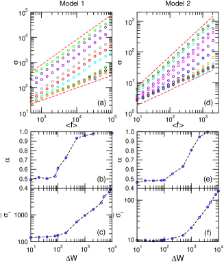
Figure 4: In Model 1 on each “day” $t$ we release $W(t)=\left<{W}\right>+\xi(t)$ walkers on randomly selected nodes and allow them to perform $M=10^{3}$ random diffusive steps, where $\xi(t)$ is a uniformly distributed random variable between $-\Delta W$ and $\Delta W$ and $\left<{W}\right>=10^{4}$. (a) The figure shows the $\sigma(\left<{f}\right>)$ curves for $\Delta W=0,20,40,80,100,200,800,1000,4000,10000$ from top to bottom. (b) The dependence of the exponent $\alpha$ on $\Delta W$, obtained by fitting the $\sigma_{i}$ versus $\left<{f_{i}}\right>$ curves shown in (a). Note that while the figure shows a gradual transition, the transition in infinite systems should be sharp. (c) Average fluctuations $\left<{\sigma_{i}}\right>$, obtained by averaging $\sigma_{i}$ over all nodes $i$ in the system, shown in function of the amplitude of the external driving force $\Delta W$. While under $\Delta W\approx 10^{2}$ the magnitude of $\left<{\sigma_{i}}\right>$ is independent of $\Delta W$, for large $\Delta W$ the fluctuations increase rapidly, indicating that the network dynamics is externally driven. (d-f) The same as in (a-c), but for Model 2, where the diffusive dynamics was replaced by message passing. $W$ was again chosen from an uniform distribution of width $\Delta W$ and average $\left<{W}\right>=10^{4}$. In all simulations we used a scale-free network  ba99 with $\gamma=3$ and $10^{4}$ nodes.

To understand the origin of the $\alpha=1$ exponent we notice that on each node the observed day to day fluctuations have two sources. For $\Delta W=0$ we have only internal fluctuations, coming from the fact that under random diffusion (or random selection of senders and receivers in Model 2) the number of walkers (messages) that visit a certain node displays day to day fluctuations. For $\Delta W\neq 0$ the fluctuations have an external component as well, as when the total number of walkers (messages) change from one day to the other, they proportionally alter the visitation of the individual nodes as well. If the magnitude of the day to day fluctuations is significant, they can overshadow the internal fluctuations $\sigma_{i}^{int}$. Indeed, if in a given time frame the total number of walkers or messages doubles, the flux on each node is expected to grow proportionally, a potentially much larger variation than the changes induced by the internal fluctuations. Therefore, for $\Delta W\neq 0$ the external driving force, determined by the time dependent $W(t)$, contributes to the daily fluctuations with a dispersion $\sigma^{dr}(\Delta W)=\sqrt{\left<{{W(t)^{2}}}\right>-\left<{W(t)}\right>^{2}}$. The total fluctuations for node $i$ are therefore given by $\sigma_{i}^{2}=\left(\sigma_{i}^{int}\right)^{2}+\left(\sigma_{i}^{ext}\right)^{2}$. As the effect of the driving force is felt to a different degree on each node, we can write $\sigma_{i}^{ext}=A_{i}\sigma^{dr}(\Delta W)$, where $A_{i}$ is a geometric factor capturing the fraction of walkers channeled to node $i$, and depends only on the position of node $i$ within the network. When $\Delta W=0$, the external component $\sigma^{dr}$ vanishes, resulting in $\sigma^{int}_{i}=a_{i}\left<{f_{i}}\right>^{1/2}$, as discussed earlier, where $a_{i}$ is an empirically determined coefficient. When $\Delta W$ is sufficiently large, so that $A_{i}\sigma^{dr}(\Delta W)\gg\sigma_{i}^{int}$, then the fluctuations on each node are dominated by the changes in the external driving force. In this limit a node’s dynamical activity mimics the changes in the external driving force, allowing us to approximate the flux at node $i$ with $f_{i}(t)=A_{i}W(t)$. In this case we have $\left<{f_{i}}\right>=A_{i}\left<{W(t)}\right>$ and $\left<{{f_{i}}^{2}}\right>={A_{i}}^{2}\left<{{W(t)}^{2}}\right>$, giving $\sigma_{i}=\sqrt{\left<{{f_{i}}^{2}}\right>-\left<{f_{i}}\right>^{2}}~{}=A_{i}\sigma^{dr}$. As $\sigma^{dr}$ and $\left<{W(t)}\right>$ are time independent characteristics of the external driving force, we find $\sigma_{i}\simeq\sigma_{i}^{ext}=\frac{\sigma^{dr}}{\left<{W(t)}\right>}\left<{f_{i}}\right>$, providing the observed coupling (1) with $\alpha=1$. Note that this derivation is independent of the network topology or the transport process, predicting that any system for which the magnitude of fluctuations in the external driving force exceeds the internal fluctuations will be characterized by an $\alpha=1$ exponent.

These calculations imply that the fluctuations on a given node can be decomposed into an internal and an external component as

$$\sigma_{i}^{2}=a_{i}^{2}\left<{f_{i}}\right>+\left(\frac{\sigma^{dr}}{\left<{W(t)}\right>}\left<{f_{i}}\right>\right)^{2}.$$ (2)

Therefore, increasing the amplitude of fluctuations $\Delta W$ should induce a change from the $\alpha=1/2$ intrinsic or endogenous to the $\alpha=1$ driven behavior. To confirm the validity of this prediction, in Figs. 4c and f we show the average fluctuation $\bar{\sigma_{i}}$ over all nodes in function of the amplitude $\Delta W$ of the driving force. For both models we find that for small $\Delta W$ values $\bar{\sigma_{i}}$ remains unchanged, as in this regime $\bar{\sigma_{i}}\sim\sigma^{int}_{i}>\sigma^{ext}_{i}$. However, after $\Delta W$ exceeds a certain threshold, $\bar{\sigma_{i}}$ changes behavior, monotonically increasing with $\Delta W$. In this second regime the fluctuations are driven by external forces, $\bar{\sigma_{i}}\sim\sigma^{ext}_{i}\sim\bar{A_{i}}\sigma^{dr}$, and according to (2) we should observe $\alpha=1$. Indeed, we find that in both models the transition from the constant to the increasing $\bar{\sigma_{i}}$ regime (Figs. 4c,f) coincides with the crossover from the $\alpha=1/2$ to $\alpha=1$ (Figs. 4b,e). Note, however, that the gradual transition observed in Figs. 4b-e from $\alpha=1/2$ to $\alpha=1$ is a numerical artifact of the fitting process: in the transition regime the $\alpha=1/2$ and $\alpha=1$ scaling coexist on the same $\sigma(\left<f\right>)$ curve, giving an exponent that is different from $1/2$ or $1$. In reality the transition between the two regimes is sharp. To understand to what degree our findings depend on the specific simulation and model details we changed the topology from scale-free ba99 to random network and from undirected to directed network, as well as altering the nature of the external fluctuations by keeping $W$ constant in Model 1 but forcing the number of steps, $M$, to play the role of the stochastic external driving force. For each version we recover the transition between the $\alpha=1/2$ and $\alpha=1$ when the amplitude of the external fluctuations exceeds a certain threshold comment .

These results indicate that the $\alpha=1/2$ exponent captures an endogenous behavior, determined by the system’s internal collective fluctuations. In the studied model internal fluctuations are rooted in the randomness in the walkers’ arrival and diffusion; on the Internet they originate in the choices users make to where and when to send a message; for the computer chip they come from the alternating utilization of the various circuits, as required by the performed computation. In contrast, the $\alpha=1$ exponent describes driven systems, in which the fluctuations of individual nodes are dominated by time dependent changes in the external driving forces. Therefore, fluctuations of World Wide Web traffic, river streams and highway traffic are driven by such external factors as daily variations in the number of Web surfers, seasonal or daily changes in precipitation or daily variations in the number of drivers, respectively.

Of the two observed exponents our derivation indicates that $\alpha=1$ is universal, being independent of the nature of the internal dynamics or the network topology. There are no firm restrictions, however, on the scaling of the internal dynamics, raising the possibility that self-organized processes could lead to collective fluctuations that are characterized by $\alpha$ exponents different from $1/2$. Empirical evidence for potential intermediate $\alpha$ values comes from ecology, where (1) describes spatial and temporal variations of populations  taylor . It is much debated, however, whether the observed scaling represent valid exponents, or only crossovers between $\alpha=1/2$ and $1$  anderson .

We are indebted to Jay Brockman and Steven Balensiefer for providing the data on the computer chip. This research was supported by grants from NSF, NIH and DOE.

References

- (1) S. Bornholdt, H.G. Schuster, Eds. Handbook of Graphs and Networks (Wiley-VCH, Berlin, 2002); S.N. Dorogovtsev, J.F.F. Mendes, Evolution of Networks: From Biological Nets to the Internet and WWW (Oxford University Press, Oxford, 2003); R. Albert, A.-L. Barabási, Rev. Mod. Phys. 74, 47 (2002); S.H. Strogatz, Nature 410 268 (2001).
- (2) A. Vazquez, R. Pastor-Satorras, A. Vespignani, Phys. Rev. E 65, 066130 (2002).
- (3) R. F. Cancho, C. Janssen, R.V. Sole, Phys. Rev E, 64, 046119 (2001).
- (4) S. Lawrence, L. Giles, Science 280, 98 (1998).
- (5) J.R. Banavar, A. Maritan, A. Rinaldo, Nature 399, 130-132 (1999); M. Cieplak, A. Giacometti, A. Maritan, A. Rinaldo, J.R. Banavar, J. Stat. Phys. 91, 1 (1998); G. Caldarelli, Phys. Rev. E 63, 21118 (2001).
- (6) A.-L. Barabási, H.E. Stanley, Fractal Concepts in Surface Growth (Cambridge University Press, Cambridge, 1995); F. Family, T. Vicsek, Eds., Dynamics of Fractal Surfaces (World Scientific, Singapore, 1991).
- (7) While Poissonian statistics explains the scaling in the random deposition model, it is not appropriate for Ethernet traffic taqqu , indicating that the Internet’s exponent is rooted in the interplay between network topology and dynamics. The exponential distribution describing waiting times is known to predict .
- (8) W.E. Leland, M.S. Taqqu, W. Willinger and D.V. Wilson, IEEE/ACM Trans. Net., 2, No. 1, 1 (1994).
- (9) A.-L. Barabási and R. Albert, Science 286, 509 (1999).
- (10) The relative strength of fluctuations can be determined independently of the scaling exponents. Such measurements indicate that for the Internet and the microchip the magnitude of the internal fluctuations is close to times larger than the magnitude of the external fluctuations. In contrast, for the other systems the internal and external fluctuations are comparable in magnitude [M. Argollo de Menezes and A.-L. Barabási, to be published].
- (11) L.R. Taylor, Nature 189, 732 (1961).
- (12) R.M. Anderson, D.M. Gordon, M.J. Crawley, M.P. Hassel, Nature 296, 245 (1982).