Interatomic potentials for atomistic simulations of the Ti-Al system

Abstract

Semi-empirical interatomic potentials have been developed for Al, $\alpha$-Ti , and $\gamma$-TiAl within the embedded atom method (EAM) formalism by fitting to a large database of experimental as well as ab-initio data. The ab initio calculations were performed by the linearized augmented plane wave (LAPW) method within the density functional theory to obtain the equations of state for a number of crystal structures of the Ti-Al system. Some of the calculated LAPW energies were used for fitting the potentials while others for examining their quality. The potentials correctly predict the equilibrium crystal structures of the phases and accurately reproduce their basic lattice properties. The potentials are applied to calculate the energies of point defects, surfaces, and planar faults in the equilibrium structures. Unlike earlier EAM potentials for the Ti-Al system, the proposed potentials provide a reasonable description of the lattice thermal expansion, demonstrating their usefulness for molecular dynamics and Monte Carlo simulations at high temperatures. The energy along the tetragonal deformation path (Bain transformation) in $\gamma$-TiAl calculated with the EAM potential is in a fairly good agreement with LAPW calculations. Equilibrium point defect concentrations in $\gamma$-TiAl are studied using the EAM potential. It is found that antisite defects strongly dominate over vacancies at all compositions around stoichiometry, indicating that $\gamma$-TiAl is an antisite disorder compound in agreement with experimental data.

I Introduction

In the recent years, intermetallics alloys based on the gamma titanium aluminide TiAl have been the subject of intense research due to their potential for applications in the aerospace and automobile industries.Kim (1994); Appel et al. (1993); Yamaguchi et al. (1996, 2000) Such alloys have an excellent oxidation and corrosion resistance which, combined with good strength retention ability and low density, make them very advanced high temperature materials. A study of fundamental properties such as the nature of interatomic bonding, stability of crystal structures, elastic properties, dislocations, grain boundaries, interfaces, as well as point defects and diffusion are therefore warranted in order to gain more insight into the behavior of these intermetallic alloys under high temperatures and mechanical loads. Over the past few years, numerous investigations, both experimental and theoretical, have been devoted to the study of such properties.Hsiung et al. (2002); Appel (2001); Mryasov et al. (1998); Simmons et al. (1998); Zhang et al. (2001); Fu and Yoo (1993); Ikeda et al. (2001); Mishin and Herzig (2000); Fu et al. (1995) Accurate ab-initio studies of the structural stability, elastic properties, and the nature of interatomic bonding have been reported for $\gamma$-TiAl as well as other stoichiometric alloys of the Ti-Al system.Hong et al. (1991, 1990); Fu (1990) However, the application of ab-initio methods to atomistic studies of diffusion, deformation, and fracture are limited due to the prohibitively large computational resources required for modeling point defects, dislocations, grain boundaries, and fracture cracks. Such simulations require large simulation cells and computationally demanding techniques such as molecular dynamics and Monte Carlo. Semiempirical methods employing model potentials constructed by the embedded atom method (EAM)Daw and Baskes (1983, 1984); Daw et al. (1993) or the equivalent Finnis-Sinclair (FS) methodFinnis and Sinclair (1984) are particularly suitable for this purpose. These methods provide a way of modeling atomic interactions in metallic systems in an approximate manner allowing fast simulations of large systems. Several studies applying these methods to a variety of properties of $\gamma$-TiAl such as planar faults, dislocations, and point defects have been reported in the literature.Simmons et al. (1997); Paidar et al. (1999a); Mishin and Herzig (2000) The effectiveness of semiempirical methods obviously depends upon the quality of the model potentials employed. Recent studiesErcolessi and Adams (1994); Kulp et al. (1993); Liu et al. (1996); Landa et al. (1998); Ferreria et al. (1999); Mishin et al. (1999); Belonoshko et al. (2000); Mishin et al. (2001); Baskes et al. (2001); Mishin et al. (2002) have shown that the incorporation of ab-initio data during the fitting of interatomic potentials can significantly enhance their ability to mimic interatomic interactions. For example, Bakes et al. Baskes et al. (2001) examined the range of interatomic forces in aluminum using model potentials and ab-initio methods. They found that potentials that included ab-initio data during the fitting procedure could reproduce ab-initio forces much more accurately than potentials fit to experimental data only.

In the present work we explore the possibility of constructing a reliable interatomic potential for the Ti-Al system. To this end, we develop EAM-type interatomic potentials for $\gamma$-TiAl and the component elements Ti and Al by fitting to a large database of experimental properties and ab-initio structural energies of these phases. The ab-initio database has been generated by density functional calculations using the linearized augmented plane wave (LAPW) method within the generalized gradient approximation (GGA) for the exchange-correlation effects. The ab-initio data are used in the form of energy-volume relations (equations of state) of various structures of Al, Ti, and $\gamma$-TiAl . The energy along the Bain transformation path between the L1₀ and B2 structures of TiAl has also been calculated in this work.

While many EAM-type potentials have been reported for Al,Ercolessi and Adams (1994); Voter and Chen (1987); Hansen et al. (1999); Mishin et al. (1999); Baskes et al. (2001) relatively few attempts have been made to create such potentials for TiPasianot and Savino (1992); Baskes and Johnson (1994); Fernandez et al. (1995) and TiAl.Farkas (1994); Rao et al. (1991, 1995); Chen et al. (1999); Wang et al. (2001); Simmons et al. (1997); Paidar et al. (1999a) Titanium, like other transition metals, cannot be expected to follow the EAM model as accurately as noble metals usually do. In contrast, Al is known to lend itself to the EAM description quite readily.Ercolessi and Adams (1994); Voter and Chen (1987); Hansen et al. (1999); Mishin et al. (1999); Baskes et al. (2001) The $\gamma$-TiAl compound is probably a borderline case. Some of the previous EAM potentials for $\gamma$-TiAl had a reasonable success in modeling lattice properties and extended lattice defects.Farkas (1994); Simmons et al. (1997); Paidar et al. (1999a) On the other hand, Paidar et al. Paidar et al. (1999b) calculated deformation paths between different structures of TiAl by an ab-initio method and with a Finnis-Sinclair potential and found only a qualitative agreement between the two calculation methods. In this work we are trying to gain a better understanding of the applicability range of the EAM model for $\gamma$-TiAl . In particular, we want explore the possibility of obtaining a high-quality EAM potential for $\gamma$-TiAl by incorporating ab-initio data into the fitting database. Our results suggest that the quality of an EAM potential can indeed be improved this way, and that the potential proposed here can be useful for atomistic simulations of $\gamma$-TiAl .

II Construction of EAM potentials

II.1 Database of fitted physical properties

We have first constructed EAM potentials for pure Al and Ti followed by fitting a cross-interaction potential Ti-Al. The database of physical properties employed in the fitting procedure consisted of two categories. The first category is comprised of experimental data for the lattice constant, $c/a$ ratio, cohesive energy, and elastic constants. For pure Al and Ti it also included the vacancy formation energy and the linear thermal expansion factors at several temperatures. The second set of properties consisted of ab-initio energy differences between various crystal structures. Such differences are necessary to ensure the correct stability of the experimentally observed ground state structures against other possible structures and to sample a large area of configuration space away from equilibrium.

The ab-initio database consists of energy versus volume ($EV$) relations for various crystal structures. For Al, $EV$ curves were computed here for the face centered cubic (fcc), hexagonal closed packed (hcp), body centered cubic (bcc), simple cubic (sc), diamond, and the L1₀ structures. The $L1_{0}$ structure of Al is a defected fcc lattice with a vacancy in the corner of each cubic unit cell. In the case of titanium, $EV$ curves were generated in Ref. Mehl and Papaconstantopoulos, 2002 for the hcp, fcc, bcc, sc, and the omega (C32) structures. For the intermetallic compound TiAl, $EV$ relations were obtained in this work for three structures: L1₀ (CuAu prototype), B2 (CsCl prototype), and B1 (NaCl prototype). Each $EV$ curve typically consists of total energies for about $20$-$30$ different volumes around the equilibrium volume. The $c/a$ ratio of the L1₀ structure has been optimized at each volume. As the ab-initio and EAM energies are at different scales, all ab-initio energies for a given element or compound of a given stoichiometry were shifted so that to match the experimental cohesive energy of the equilibrium ground state structure. This procedure is followed merely to facilitate the comparison of structural energies calculated by different methods and does not introduce any new approximation. The equilibrium energy of the D0₁₉-Ti₃Al compound has also been calculated here to check the methodology and provide useful reference information. The energy of this phase was minimized with respect to its volume while keeping the $c/a$ ratio fixed at the value found in Ref. Watson and Weinert, 1998.

The $EV$ curves were calculated using the full potential LAPW methodAnderson (1975); Wei and Krakauer (1985); Singh (1994) within the Hohenberg-Kohn-Sham formulation of the density functional theory.Hohenberg and Kohn (1964); Kohn and Sham (1965); Parr and Yang (1989) The calculations were carried out in a spin-restricted mode and the exchange-correlation effects were treated at the level of the GGA. The $EV$ calculations for Ti were carried out using an LAPW code available at the Naval Research Laboratory and were reported in Ref. Mehl and Papaconstantopoulos, 2002. The calculations for Al, TiAl and Ti₃Al were performed in this work and employed the WIEN2K package.Blaha et al. (2002) The Perdew-WangPerdew (1991); Perdew et al. (1992, 1993) (PW91) exchange-correlation functional was used for Ti calculations,Mehl and Papaconstantopoulos (2002) while its simplified and more efficient version referred to in literature as PBEPerdew et al. (1996) was used for Al and TiAl. The muffin-tin radii of Al and Ti were chosen to be 2 a.u. For each crystal structure, systematic k point and basis set convergence tests were carried out at a fixed volume near equilibrium volume. The same set of parameters was subsequently employed for different volumes as well as for the Bain path calculations. The accuracy of the LAPW total energies calculated in the present work was estimated to be better than 0.5 mRy/atom.

We now describe some relevant details of the potential fitting procedure. In the embedded atom formalism,Daw and Baskes (1983, 1984) the total energy of a system is expressed as

$$E_{tot}=\frac{1}{2}\sum_{i,j}\Phi_{ij}(r_{ij})+\sum_{i}F_{i}(\bar{\rho_{i}}).$$ (1)

Here, $\Phi_{ij}$ is the pair-interaction energy between atom $i$ and $j$ at positions $\vec{r}_{i}$ and $\vec{r}_{j}$, and $F_{i}$ is the embedding energy of atom $i$. The $\bar{\rho}_{i}$ in Eq. (1) is the host electron density at site $i$ induced by all other atoms in the system. The latter is given by

$$\bar{\rho_{i}}=\sum_{j\neq i}\rho_{j}(r_{ij}).$$ (2)

For a binary system A-B, the total energy given by Eq. (1) is invariant with respect to the following set of transformations:Johnson (1989); Mishin et al. (2002)

$$\rho_{A}(r)\rightarrow s_{A}\rho_{A}(r),$$ (3)

$$\rho_{B}(r)\rightarrow s_{B}\rho_{B}(r),$$ (4)

$$F_{A}(\bar{\rho})\rightarrow F_{A}(\rho_{A}(r)/s_{A}),$$ (5)

$$F_{B}(\bar{\rho})\rightarrow F_{B}(\rho_{B}(r)/s_{B}),$$ (6)

$$F_{A}(\bar{\rho})\rightarrow F_{A}(\bar{\rho})+g_{A}\bar{\rho},$$ (7)

$$F_{B}(\bar{\rho})\rightarrow F_{B}(\bar{\rho})+g_{B}\bar{\rho},$$ (8)

$$\Phi_{AA}(r)\rightarrow\Phi_{AA}(r)-2g_{A}\rho_{A}(r),$$ (9)

$$\Phi_{BB}(r)\rightarrow\Phi_{BB}(r)-2g_{B}\rho_{B}(r),$$ (10)

$$\Phi_{AB}(r)\rightarrow\Phi_{AB}(r)-2g_{A}\rho_{A}(r)-2g_{B}\rho_{B}(r),$$ (11)

where $A$ and $B$ refer to the type of element (Al or Ti) and $s_{A},s_{B},g_{A},\mbox{\,and\,}g_{B}$ are arbitrary constants. For any particular compound, the potential can be cast into the so-called effective pair formatJohnson (1989) by choosing $g_{A}=-F^{\prime}_{A}(\bar{\rho_{A}}^{0})$ and $g_{B}=-F^{\prime}_{B}(\bar{\rho_{B}}^{0})$, where $\bar{\rho_{A}}^{0}$ and $\bar{\rho_{B}}^{0}$ are the equilibrium electron densities on atoms in the compound. The effective pair format provides a convenient way of comparing different potentials for the same compound.

An EAM potential for a binary system can be constructed by two different procedures. One is to optimize all potential functions simultaneously during a single fit, as it was done for example for the Ni-Al system.Mishin et al. (2002) This scheme offers the advantage of having many parameters available for fitting to properties of a selected alloy or compound. However, it suffers from the drawback that the quality of potentials for pure elements (Al and Ti in our case) is often poor. An alternative and more common approach is to separately develop accurate EAM potentials for pure elements and use them to fit the cross potential for alloys (compounds). We resort to the latter procedure for the Ti-Al system. The parametrization of potential functions employed in the fitting procedure is discussed below.

II.2 EAM potential for Al

For the EAM potential for Al, we chose the electron density function in the form

$$\rho(r)=\psi\biggl{(}\frac{r-r_{c}}{h}\biggr{)}\Bigl{\{}A_{0}(r-r_{0})^{y}e^{-\gamma(r-r_{0})}$$

$$\times~{}\Bigl{(}1+B_{0}\,e^{-\gamma(r-r_{0})}\Bigr{)}+C_{0}\Bigr{\}},$$ (12)

Here, $A_{0},B_{0},C_{0},r_{0},r_{c},h,y\mbox{ and }\gamma$ are the fitting parameters and $\psi(x)$ is a cutoff function defined as

$$\psi(x) = 0~{}~{}{for~{}~{}}x\geq 0$$ (13)

$$= \frac{x^{4}}{(1+x^{4})}~{}~{}{for~{}~{}}x<0,$$

where $r_{c}$ is the cutoff distance. The electron density in equilibrium fcc Al is normalized to unity, i.e. $\bar{\rho}=\sum_{j}N_{j}\rho_{j}=1$ , where $j$ runs over coordination shells and $N_{j}$ is the number of atoms on the $j$-th coordination shell. This constraint fixes one parameter in the above set of parameters. The pair interaction function is parametrized in the form

$$\Phi(r)=\Biggl{[}\frac{V_{0}}{(b_{2}-b_{1})}\biggl{(}\frac{b_{2}}{z^{b_{1}}}-\frac{b_{1}}{z^{b_{2}}}\biggr{)}+\delta\Biggl{]}\psi\biggl{(}\frac{r-r_{c}}{h}\biggr{)},$$ (14)

where, $z=r/r^{\prime}$, and $b_{1}$, $b_{2}$, $\delta$, $V_{0}$, and $r^{\prime}$ are fitting parameters. Thus, altogether we have $12$ fitting parameters for functions $\rho(r)$ and $\Phi(r)$.

The embedding energy is obtained by equating the energy of fcc Al [Eq. (1)] to the universal equation of state (EOS). By studying a broad range of materials, Rose et al. Rose et al. (1984) proposed the “universal” EOS in the form

$$E(r)=-E_{0}\bigl{[}1+\alpha(r/r_{e}-1)\bigr{]}e^{-\alpha(r/r_{e}-1)},$$ (15)

where $\alpha=\sqrt{9\Omega_{0}B/E_{0}}$, and $r$, $E_{0}$, $\Omega_{0}$, $B$, $r_{e}$ are the nearest-neighbor distance, cohesive energy, equilibrium atomic volume, the bulk modulus, and the equilibrium-nearest neighbor distance, respectively. It is generally found that the EAM potentials which exactly follow Rose’s EOS [Eq. (15)] underestimate energies at high pressures.Mishin et al. (2002) We have therefore modified Eq. (15) to allow for a more accurate fit to energies at high pressures. The modified equation has the form

$$E(r)=-E_{0}\Biggl{[}1+\alpha x+\beta\alpha^{3}x^{3}\frac{2x+3}{(x+1)^{2}}\Biggr{]}e^{-\alpha x},$$ (16)

with $x=(r/r_{e}-1)$. The parameter $\beta$ in this equation is related to the pressure derivative of the bulk modulus at equilibrium as $B_{0}^{\prime}=\frac{2}{3}\alpha+6\alpha\beta+2$. This modification does not alter the exact fitting of the potential to $E_{0},r_{e}$ and $B$ but provides a way to achieve an accurate fit to the experimental pressure-volume relation by adjusting the value of $\beta$.

II.3 EAM potential for Ti

Titanium has the hcp structure at $T=0$ ($\alpha$-Ti phase). For hcp metals, an EAM potential can only be fitted to elastic constants $C_{ij}$ if the relation $(3C_{12}-C_{11})/2>(C_{13}-C_{44})$ is satisfied.Pasianot and Savino (1992) Fortunately, this relation holds for $\alpha$-Ti.

In the present EAM potential for Ti, the electron density function is described by

$$\rho(r)=\Biggl{[}Ae^{-\alpha_{1}(r-r_{0})^{2}}+e^{-\alpha_{2}(r-r_{0}^{\prime})}\Biggr{]}\psi\biggl{(}\frac{r-r_{c}}{h}\biggr{)},$$ (17)

where the cutoff function $\psi(x)$ is given by Eq. (13) with the fitting parameters $A,\alpha_{1},\alpha_{2},r_{0},r_{0}^{\prime},r_{c}$, and $h$. One of the parameters is fixed by the normalization condition $\bar{\rho}=1$ at equilibrium.

The pair interaction function is represented by

$$\Phi(r_{ij})=\psi\biggl{(}\frac{r-r_{c}}{h}\biggr{)}\biggl{\{}V_{0}\,e^{-\beta_{1}r_{1}}+V_{0}^{\prime}\Bigl{[}e^{-2\beta_{2}(r-r_{1}^{\prime})}-2\,e^{\beta_{2}(r-r_{1}^{\prime})}\Bigr{]}+\delta\biggr{\}},$$ (18)

where $V_{0},V_{0}^{\prime},\beta_{1},\beta_{2},r_{1},r_{1}^{\prime},\mbox{\,and\,}\delta$ are fitting parameters. The embedding energy function is expressed as a polynomial:

$$F(\bar{\rho}) = F_{0}+\frac{1}{2}F_{2}(\bar{\rho}-1)^{2}+q_{0}(\bar{\rho}-1)^{3}$$ (19)

$$+~{}\sum_{i=1}^{3}B_{i}(\bar{\rho}-1)^{i+3}.$$

Here $F_{0}$ and $F_{2}$ are the embedding energy and its second derivative at equilibrium, respectively. These can be expressed in terms of the experimental values of $E_{0}$, $B$, and $\Omega_{0}$:

$$F_{0}=E_{0}-\frac{1}{2}\sum_{j}N_{j}\Phi_{j}$$

and

$$\frac{1}{2}\sum_{j}N_{j}\Phi^{\prime\prime}_{j}R^{2}_{j}+F_{2}\Bigl{(}\sum_{j}N_{j}\rho_{j}R_{j}\Bigr{)}^{2}=9B\Omega_{0},$$

where $j$ runs over coordination shells, $N_{j}$ is the number of atoms on the $j$-th coordination shell of radius $R_{j}$, while $\Phi_{j}$ and $\Phi_{j}^{\prime\prime}$ are the pair interaction energy and its second derivative evaluated at $R_{j}$. The coefficients $q_{0}$ and $B_{i}~{}(i\leq 3)$ in Eq. (19) are fitting parameters. The parameter $q_{0}$ was adjusted to ensure that the embedding energy vanishes when the electron density goes to zero, that is, $F(0)=0$. This requirement leads to the following expression for $q_{0}$:

$$q_{0}=F_{0}+\frac{F_{2}}{2}+B_{1}-B_{2}+B_{3}.$$ (20)

During the optimization of fitting parameters, the energy of the hcp structure was required to approximately follow the Rose’s EOS [Eq. (15)] in the neighborhood of equilibrium. This was achieved by adding to the objective function the mean-squared deviation of the energy from Eq. (15) at several points near the equilibrium.

II.4 The cross potential Ti-Al and the fitting procedure

Once the EAM potentials for Al and Ti are obtained, the cross potential representing the interactions between Ti and Al atoms was constructed by employing the parametrization given by Eq. (14). The transformation coefficients $s_{Al},g_{Ti},$ and $g_{Al}$ [see Eqs. (3)-(11)] were used as additional adjustable parameters.

It should be mentioned that the specific analytical forms of the potential functions adopted in this work were found by trying a number of different forms and selecting those which provided a better accuracy of fitting with less parameters. The optimized values of the fitting parameters are listed in Table 1. The potential functions are plotted in Fig. 1 in the effective pair formatMishin et al. (2002); Johnson (1989) with respect to $\gamma$-TiAl . These functions are available in the tabulated form on InternetNRL or from the authors upon request. The cutoff radii of atomic interactions in Al, Ti, and TiAl are 6.72, 5.19, and 5.77 Å, respectively. The fitting procedure involves the total of $39$ independent fitting parameters.

III Tests and Applications of the potentials

III.1 Aluminum

The accuracy of the fitted EAM potential for Al can be adjudged from Table 2, wherein the basic lattice properties, elastic constants, vacancy formation and migration energies, surface energies, and the stacking fault energy predicted by the potential are compared with their experimental values. We have also included the results obtained with our previous EAM potential for Al,Mishin et al. (1999) which we hereafter refer to as MFMP. The results obtained with the new EAM potential are in good agreement with their experimental counterparts. The calculated vacancy formation energy $E^{f}_{v}$ and migration energy $E^{m}_{v}$, which are important for studying point defect diffusion, are well reproduced. The calculated vacancy formation volume $\Omega_{v}^{f}$ compares well with the one obtained with the MFMP potential as well as with experimental data.Emrick and McArdle (1969) The predicted intrinsic stacking fault $(\gamma_{SF})$ energy is on the lower end of the range of experimental values while the ab initioKaxiras (1997, 2000) calculatations yeilds a higher value of 166 mJ/m² . The calculated symmetrical twin boundary $(\gamma_{T})$ energy is in good agreement with its experimental counterpart. The unstable stacking fault energy is underestimated with respect to the ab initioKaxiras (1997, 2000) value of 220 mJ/m² . The surface energies are underestimated in comparison with experiment, which is a general characteristic of EAM potentials.

The structural energy differences for Al, given in Table 3, reproduce ab-initio energies reasonably accurately. The EAM potential predicts the $c/a$ ratio of the hcp structure to be 1.63 in good agreement with the optimized value of 1.645 obtained by the LAPW calculations. In agreement with earlier findings,Mishin et al. (1999) bcc Al is mechanically unstable ($C_{11}<C_{12}$) and transforms to the fcc structure upon $c/a$ relaxation. The sc structure is also mechanically unstable with $C_{44}<0$. A comparison of the EOS’s of various crystalline structures of Al calculated with the EAM potential and by the LAPW method is presented in Fig. 2. The EAM curves are seen to agree with the LAPW results fairly well. The agreement is particularly good for the bcc and fcc structures over a large range of volumes, but tends to worsen for more open structures.

As was mentioned in Section II B, the Al potential was fit to the experimental $P(V)$ relation by adjusting the parameter $\beta$ in the generalized EOS, Eq. (16). The optimized value of $\beta=0.00489$ provides an excellent agreement with experimental data up to pressures of about 700 GPa, as illustrated in Fig. 3. In contrast, the standard Rose’s EOS ($\beta=0$) underestimates the pressures under strong compressions. Note that both equations share the same values of $E_{0}$, $B$ and $a_{0}$. The excellent fit to high pressure data makes the potential useful for simulating shock waves, sputter deposition, and other processes involving a close approach of atoms.

Thermal expansion of Al was studied within the temperature range of $5$-$1000$ K. The calculated thermal expansion factors at selected temperatures are given in Table 4. They were obtained using a 864-atom supercell by two different methods. In the first method, the free energy of the crystal was minimized as a function of volume in the quasiharmonic approximation.Foiles (1994) This method includes quantum-mechanical effects such as zero-point vibrations and should yield more accurate values of the thermal expansion factor at low temperatures. However, it may not be very accurate at high temperature where the anharmonic effects become significant. The second type of calculation was carried out by the Metropolis Monte Carlo method.Foiles (1994); Foles and Adams (1989) This method is based on classical mechanics and fully incorporates anharmonic effects. It is therefore more adequate for thermal expansion calculations at high temperatures. As can be seen from Table 4, the MC results are quite close to experimental data at high temperatures.

Overall, the EAM potential developed here provides a good description of a wide range of Al properties. Despite the existence of other high-quality EAM potentials for Al in the literature,Ercolessi and Adams (1994); Hansen et al. (1999); Mishin et al. (1999) we chose not to re-use one of them but rather generate a new potential so that to have all potential functions for the Ti-Al system created by the same methodology. We also used this work as an opportunity to address some weak points of previous potentials. For example, even though the MFMP potentialMishin et al. (1999) demonstrates a better agreement with experiment for some of the properties listed in Table 2, the present potential describes the thermal expansion and high-pressure behavior of Al more accurately. The present potential is also based on a larger set of ab-initio data and should be better transferable to configurations away from equilibrium. It should also be mentioned that the use of smooth analytical functions in this work makes the potential more robust in comparison with the cubic-spline parameterization applied in Ref. Mishin et al., 1999.

III.2 Titanium

Equilibrium lattice properties, vacancy characteristics, as well as stacking fault and surface energies in Ti computed using the present EAM potential are compared with experimental data in Table 5. We have also included the results obtained with the EAM potential developed by Fernandez et al. ,Fernandez et al. (1995) which will be referred to as FMP. The latter is an improved version of the potential proposed in Ref. Pasianot and Savino, 1992. Although our potential was not fitted to the $c/a$ ratio exactly, the predicted value of 1.585 is in a good agreement with the experimental value of 1.588. The elastic constants are also reproduced reasonably well.

The vacancy formation energy $E_{v}^{f}$ was fitted to the target value of $1.85$ eV. The experimental value of $E_{v}^{f}$ reported by ShestopalShestopal (1966) is $1.55$ eV, more recent positron annihilations measurementsHashimoto et al. (1984) give $E_{v}^{f}=1.27$ eV, while the ab-initio linearized muffin-tin orbital method (LMTO) methodBacq et al. (1999) yields a much higher value of $2.14$ eV. We therefore opted to fit to an intermediate value of $1.85$ eV, which after the relaxation decreased to $1.83$ eV. The vacancy migration energy $E^{m}_{v}$ was calculated using the nudged elastic band method.Jonsson et al. (1998) In the hcp lattice with a nonideal $c/a$ ratio, the basal and non-basal vacancy jumps are not identical. The calculated values of $E_{v}^{m}$ for the basal and non-basal jumps are $0.80$ eV and $0.83$ eV, respectively. The FMP potential gives smaller values of $0.51$ eV and $0.48$ eV, respectively. While the experimental value of the vacancy formation energy is rather uncertain, the experimental activation energy $Q$ of self-diffusion in $\alpha$-Ti , which is the sum of $E_{v}^{f}$ and $E_{v}^{m}$ , has been measured fairly accurately.Koppers et al. (1997) For self-diffusion perpendicular to the $c$ axis, the experimental value is $Q=3.14$ eV. The present EAM potential predicts $Q=2.62$ eV, while the FMP potential gives a lower value of $2.02$ eV.

There are three stacking faults on the basal plane in $\alpha$-Ti , which are deviations from the normal stacking sequence ${ABABAB}$ of closed packed planes in the hcp structure.Hull and Bacon (1989); Hirth and Lothe (1982) The intrinsic fault $I_{1}$ is formed by a removal of one hexagonal layer followed by a $\frac{1}{3}<10\bar{1}0>$ translation of all atoms above this fault. The resultant stacking sequence is

$$I_{1}:~{}~{}\,\,ABAB{|}CBCBC,$$

where the vertical bar indicates the position of the fault. The intrinsic stacking fault $I_{2}$ is created by a $\frac{1}{3}<10\bar{1}0>$ slip:

$$I_{2}:~{}~{}\,\,ABAB|CACAC.$$

The extrinsic stacking fault $E$ result from the insertion of an extra hexagonal plane into the normal stacking sequence:

$$I_{E}:~{}~{}\,\,ABAB{|}C{|}ABAB.$$

The calculated relaxed stacking fault energies (Table 5) compare well with those obtained with the FMP potential. The experimental value of the $I_{2}$ fault energy is about $300$ mJ/m² and is considered to be a rough estimate. Both EAM potentials underestimate this experimental value. All our efforts to obtain a higher $\gamma_{I_{2}}$ value during the fitting of the present potential did not have much success. In fact, any attempt to raise $\gamma_{I_{2}}$ above $66$ mJ/m² resulted in a deterioration of other properties, which gave us an indication that higher stacking fault energies may be beyond the capabilities of the EAM. Note, however, that the EAM-predicted stacking fault energies follow the expected relation:Hull and Bacon (1989) $\gamma_{E}\approx\frac{3}{2}\gamma_{I_{2}}\approx 3\gamma_{I_{1}}$. The limited success in fitting to higher stacking fault energies is likely to be due to the directional component of bonding in Ti owing to d electrons. The covalent nature of bonding cannot be described by the central-force-based EAM model. More rigorous parameter-based methods such as the modified EAM,Baskes and Johnson (1994); Baskes (1992) bond order potentialsAkoi (1993); Akoi and Pettifor (1994); Girshick et al. (1998) or the tight-binding method,Mehl and Papaconstantopoulos (1996) which include angular-dependent interactions, may give higher stacking fault energies.

The predicted value of the $(0001)$ surface energy, $1725$ mJ/m² , slightly underestimates the experimental value. This is again consistent with the general trend of the EAM to underestimate surface energies. The FMP potential yields an even smaller value of $1439$ mJ/m² , whereas the ab-initio surface energies, $2100$ mJ/m² (Ref. de Boer et al., 1988) and 1920 mJ/m² (Ref. Tyson and Miller, 1977), overestimate the experimental value.

The LAPW and the EAM energies of various crystal structures of Ti relative to the hcp structure are reported in Table 6. We note that the LAPW calculations predict the omega structure to be the ground state, with the hcp energy being 0.06 eV/atom higher. We have, therefore, excluded the omega structure from the fitting procedure. Overall, both EAM potentials yield similar energy differences between the structures, with the present potential performing somewhat better. Both potentials predict the hcp structure to be more stable than the omega structure in agreement with experiment. In Fig. 4, the EOS’s of the hcp, fcc, bcc, and the sc structures of Ti calculated with the present EAM potential are compared with the LAPW results. The agreement between the two calculation methods is good for the close-packed structures but becomes poorer for the low coordinated sc structure. In the latter case, however, the present EAM potential is closer to the LAPW data than the FMP potential.

The linear thermal expansion of Ti was calculated within the quasiharmonic approximation and by the MC method using a supercell with 800 atoms. The $c/a$ ratio was kept fixed at its equilibrium $T=0$ value during the calculations. The obtained values of the thermal expansion factor for selected temperatures are reported in Table 7. The agreement with experimental dataTouloukian et al. (1975) for polycrystalline Ti is reasonable. The FMP potential gives a poorer agreement with experiment. For example, at 293 K the FMP potential gives the quasiharmonic linear thermal expansion of 1.35% while the experimental value is 0.15%.

III.3 Intermetallic compound $\gamma$-TiAl

The physical properties of $\gamma$-TiAl obtained with the present EAM potential are summarized in Table 8. The lattice constant and the cohesive energy are reproduced accurately. The $c/a$ ratio is correctly predicted to be larger than unity and is in good agreement with the experimental value. The elastic constants are in a reasonable agreement with experiment, the root-mean-squared deviation for elastic constants being about 22%. We note that the negative signs of the two Cauchy pressures, ($C_{12}-C_{66}$) and ($C_{13}-C_{44}$), are not reproduced by the present potential, nor are they reproduced by previous EAM-type potentials. The negative Cauchy pressures in TiAl are caused by the directional component of bonding and cannot be described by the EAM. Table 8 also includes the numbers calculated with the Farkas potentialFarkas (1994); Far as well as with the P₂ potential constructed by Simmons et al. Simmons et al. (1997) The respective root-mean-squared deviations of the elastic constants from experimental data are 45% and 28%.

The planar defect energies in $\gamma$-TiAl are summarized in Table 9. They were calculated using supercells with an effective cubic lattice with the lattice parameter $a=\left(a_{0}^{2}c_{0}\right)^{1/3}$ and without volume relaxation. Since the cohesive energy of the equilibrium tetragonal lattice was used as a reference in the calculations, the resultant fault energies can be slightly overestimated. For the superlattice intrinsic stacking fault (SISF), the EAM value of $173$ mJ/m² is slightly higher than the experimental value of $140$ mJ/m² . There have been a number of ab-initio calculations of the SISF energy with results scattered over the range of $90$-$172$ mJ/m² . For the complex stacking fault (CSF) energy we obtain the value of $299$ mJ/m² well bracketed between ab-initio results. Experimental data for the CSF energy are not available. The calculated value of the antiphase boundary (APB) energy, $266$ mJ/m² , is also in a good agreement with the experimental value of $250$ mJ/m² . The ab-initio APB energies are scattered over the wide range $510$-$670$ mJ/m² . The hierarchy of planar fault energies in $\gamma$-TiAl was investigated by Wiezorek and Humphreys.Wiezorek and Humphreys (1995) According to their preliminary computational results, this hierarchy in Ti-$54$at%Al is $\gamma_{CSF}>\gamma_{APB}>\gamma_{SISF}$. The present EAM potential predicts the same ordering. On the other hand, ab-initio calculations with the linearized Korringa-Kohn-Rostoker (LKKR) methodWoodward et al. (1992) and the full potential LAPW (FLAPW) methodFu and Yoo (1990) give the $\gamma_{APB}>\gamma_{CSF}>\gamma_{SISF}$ ordering. More recent calculations by Ehmann and Fähnle by the LAPW method including local atomic relaxations are consistent with the latter ordering of the stacking fault energies. The discrepancy between the experimental data and EAM calculations, on one hand, and ab-initio calculations, on the other hand, originates primarily from the high APB energy delivered consistently by ab-initio methods. The low APB energy observed experimentally may reflect the local disorder near the APB taking place due to the off-stoichiometry and/or temperature effects. The similarly low APB energy predicted by the present EAM potential can lead to a good agreement between atomistic simulations and experiment.

Simmons et al. Simmons et al. (1997) succeeded in generating a set of EAM potentials for $\gamma$-TiAl fit to high APB energies comparable to ab-initio values, but their potentials give $c/a<1$ in contradiction to experimental data. When generating our potential we could also achieve higher $\gamma_{APB}$ values at the expense of $c/a<1$, but could never increase $\gamma_{APB}$ above $266$ mJ/m² while keeping $c/a>1$ and maintaining a good quality of fit to other properties. We believe that the underestimation of the APB energy is another intrinsic limitation of the central-force EAM as applied to $\gamma$-TiAl . FarkasFarkas (1994) constructed a potential that gives $\gamma_{APB}>\gamma_{CSF}$ while $c/a>1$. However, some of the elastic constants predicted by that potential are in a poor agreement with experimental data, especially $C_{13}$ and $C_{33}$ (cf. Table 8). The potential also gives a discontinuous temperature dependence of the quasiharmonic thermal expansion, with unrealistically large values at high temperatures.

The $EV$ curves computed with the present EAM potential and by the LAPW method are presented in Fig. 5. The agreement between the two calculation methods is good for the L1₀ structure. The difference between the two curves for the B2 and B1 structures is presumably due to the limited accuracy of the EAM method to describe the open structures. The formation energies for different structures of TiAl (relative to fcc Al and hcp Ti) calculated by the LAPW method and with the present EAM potential are presented in Table 10. For comparison, experimental and ab-initio results available in the literature have also been included in the Table. The formation energies obtained with the present EAM potential are in good agreement with the corresponding experimental and ab-initio energies. The L1₀ structure is correctly produced to be the ground state. We note the $B2$ and $B32$ structures are unstable with respect to the $c/a$ optimization. In particular, the $B2$ structure transforms to the equilibrium L1₀ phase upon $c/a$ relaxation.

For Ti₃Al , the EAM potential correctly predicts the DO₁₉ structure to be the equilibrium ground state of Ti₃Al (Table 10). The lattice constants, cohesive energy, and the elastic constants of D0₁₉-Ti₃Al are given in Table 11. We emphasize that none of these properties were included in the potential fit. The observed agreement with experimental data demonstrates a good transferability of our potential.

The EAM potential was also applied to investigate the Al₃Ti compound. Experimentally, the equilibrium structure of Al₃Ti is DO₂₂. The present EAM potential predicts the L1₂ structure to be $0.01$ eV lower in energy than the DO₂₂ structure, suggesting that the potential may not suitable for simulating the Al₃Ti compound.

Thermal expansion factors of $\gamma$-TiAl calculated within the quasiharmonic approximation and by the Monte Carlo method are presented in Table 12. The calculated values are in agreement with those estimated from Fig. 4 in Ref. Zupan and Hemker, 2001.

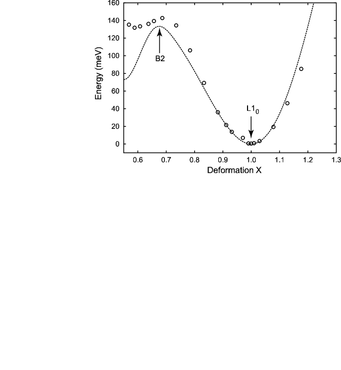
Figure 6: Energy per atom as a function of the deformation parameter X (see text for details) along the volume conserving tetragonal deformation path (Bain path) in TiAl. The energy is given relative to the equilibrium $L1_{0}$ structure. The dotted line is predicted by the present EAM potential and the symbols represents the LAPW results.

The energy along the Bain path between the tetragonal $\gamma$-TiAl structure and the B2 structure was calculated by the EAM and LAPW methods. Starting from the equilibrium tetragonal $\gamma$-TiAl structure, the $c/a$ ratio was varied by keeping the volume constant. The energy change during the transformation is plotted in Fig. 6 as a function of the deformation parameter $X$ defined by $c/a=X(c_{0}/a_{0})$. The EAM energies are observed to closely follow the LAPW energies along the path. This agreement confirms a good transferability of the present EAM potential.

Point defect properties play an important role in the atomic disorder and diffusion in $\gamma$-TiAl . The TiAl lattice supports two types of vacancy (V_Ti and V_Al) and two types of antisite defects (Ti atom on the Al sublattice, Ti_Al, and Al atom on the Ti sublattice, Al_Ti).Mishin and Herzig (2000) The so-called “raw” formation energies and entropiesMishin and Herzig (2000) of the defect formation have been calculated with the present EAM potential using the molecular statics method for the energies and the quasiharmonic approximation for the entropies.

When analyzing point defects in ordered compounds it is more convenient to deal with hypothetical composition-conserving defect complexes rather than individual defects.Mishin and Herzig (2000); Hagen and Finnis (1998); Korzhavyi et al. (2000); Meyer and Fähnle (1999) It should be emphasized that the defects are grouped into complexes conceptually and not physically. The complexes are assumed to be totally dissociated and interactions between their constituents are neglected. The advantage of dealing with composition-conserving complexes is that all reference constants involved in their energies and entropies cancel out. This allows us to directly compare results obtained by different calculation methods. The complex energies and entropies can be expressed in terms of the “raw” energies $\epsilon_{d}$ and entropies $s_{d}$, $d$ = V_Ti, V_Al, Ti_Al, Al_Ti.Mishin and Herzig (2000) The expressions for some of the complex energies are given in Table 13. Similar expressions hold for the complex entropies, except that the cohesive energy $E_{0}$ should be replaced by the perfect lattice entropy per atom. Table 13 summarizes the results of the EAM calculations for several defect complexes and compares them with the ab-initio energies reported by Woodward et al. Woodward et al. (1998) The agreement between the two calculation methods is reasonable. We emphasize again that point defect properties of $\gamma$-TiAl were not included in the potential fit.

Using the complex energies and entropies, the equilibrium defect concentrations have been calculated as functions of the bulk composition around the stoichiometry within the lattice gas model of non-interacting defects.Mishin and Herzig (2000); Hagen and Finnis (1998); Korzhavyi et al. (2000); Meyer and Fähnle (1999) Fig. 7 shows the calculation results for $T=1000$ K. We see that all compositions are strongly dominated by antisite defects. This observation is well consistent with the experimentally established fact that $\gamma$-TiAl is an antisite disorder compound.Elliot and Rostoker (1954); Brossmann et al. (1994); Shirai and Yamaguchi (1992) The vacancy concentrations are several orders of magnitude smaller than antisite concentrations. In the stoichiometric composition, most of the vacancies reside on the Ti sublattice. All these features have been observed at all temperatures in the range 800-1200 K.

IV Summary

EAM potentials have been developed for Al, $\alpha$-Ti and $\gamma$-TiAl by fitting to a database of experimental data and ab-initio calculations. The potentials have been tested against other experimental and ab-initio data not included in the fitting database. The ab-initio structural energies for Ti were calculated previously,Mehl and Papaconstantopoulos (2002) while those for Al and Ti-Al compounds have been generated in this work. All these calculations employed the full-potential LAPW method within the GGA approximation. Besides serving for the development of the EAM potentials, the obtained ab-initio energies are also useful as reference data for the Ti-Al system.

The Al potential is fit to the target properties very accurately and has demonstrated a good performance in the tests. It has certain advantages over the previously developed potential,Mishin et al. (1999) particularly with respect to the lattice thermal expansion and the pressure-volume relation under large compressions. The fit of the Ti potential is less successful, presumably because of the directional component of interatomic bonding that is not captured by the central-force EAM model. In particular, the potential underestimates the stacking fault energies on the basal plane. Further improvements of the potential do not appear to be possible within the EAM. This potential can be viewed as a supporting potential for the Ti-Al system, but we also believe that it can be useful in atomistic simulations in pure Ti where subtle details of atomic interactions may not be critical. Since the potential is fit reasonably well to the elastic constants, thermal expansion factors and the vacancy formation energy, it can be employed for modeling diffusion and creep in large systems that are not accessible by more accurate, yet slower, ab-initio methods.

For the $\gamma$-TiAl compound, the potential developed here reproduces reasonably well the basic lattice properties, planar fault energies, as well as point defect characteristics. The fit to the elastic constants is better than with previous potentials. However, the negative Cauchy pressures in $\gamma$-TiAl have not been reproduced by the present nor previous EAM potentials. The planar fault energies calculated with the potential are in a good agreement with experiment, but the APB energy is lower than all ab-initio values. The fit to ab-initio energies of alternative structures of TiAl enhances the transferability of the potential to configurations away from equilibrium. This fact is verified by the good agreement between the EAM and LAPW energies along the Bain transformation path. The potential also correctly predicts the equilibrium DO₁₉ structure of Ti₃Al and gives a fairly good agreement with experiment for the cohesive energy, lattice parameters, and elastic constants of this compound. The point defect energies and entropies in $\gamma$-TiAl calculated with the potential are in agreement with the antisite disorder mechanism established for this compound experimentally. We emphasize that neither the Bain path nor any information on Ti₃Al or point-defect properties in $\gamma$-TiAl were included in the fitting database. This success of the proposed potential points to its ability to describe atomic interactions in the Ti-Al system on a reasonable quantitative level. The potential should be suitable for large-scale atomistic simulations of plastic deformation, fracture, diffusion, and other processes in $\gamma$-TiAl . At the same time we acknowledge that more rigorous models, particularly those including angular-dependent interactions, are needed for addressing the negative Cauchy pressures, high APB energy, and other properties of $\gamma$-TiAl that lie beyond the capabilities of the EAM.

Table 1: Optimized values of the fitting parameters of the EAM potential for the Ti-Al system.

Al		Ti		TiAl
Parameter	Optimal value	Parameter	Optimal value	Parameter	Optimal value
$r_{c}$ (Å)	6.724884	$r_{c}$ (Å)	5.193995	$r_{c}$ (Å)	5.768489
$h$ (Å)	3.293585	$h$ (Å)	0.675729	$h$ (Å)	0.619767
$V_{0}$ (eV)	$-$3.503182 $\times~{}10^{3}$	$V_{0}$ (eV)	$-$3.401822 $\times~{}10^{6}$	$V_{0}$ (eV)	$-$0.737065
$r^{\prime}$(Å)	2.857784	$r_{1}$ (Å)	$-$8.825787	$r_{0}$ (Å)	2.845970
$b_{1}$	8.595076 $\times~{}10^{-2}$	$\beta_{1}$ (1/Å)	5.933482	$b_{1}$	5.980610
$b_{2}$	5.012407 $\times~{}10^{-2}$	$V_{0}^{\prime}$ (eV)	0.161862	$b_{2}$	5.902127
$\delta$(eV)	3.750298 $\times~{}10^{3}$	$r_{1}^{\prime}$(Å)	3.142920	$\delta$ (eV)	0.078646
$y$	2.008047 $\times~{}10^{1}$	$\beta_{2}$ (1/Å)	2.183169	$s_{Al}$	0.951039
$\gamma$(1/Å)	4.279852	$\delta$	$-$0.601156 $\times~{}10^{-1}$	$g_{Ti}$ (eV)	4.839906
$B_{0}$(Å)	1.192727 $\times~{}10^{5}$	$A$	3.656883 $\times~{}10^{2}$	$g_{Al}$ (eV)	1.281479
$C_{0}$ (1/Å3)	8.60297 $\times~{}10^{-2}$	$r_{0}$ (Å)	$-$1.169053 $\times~{}10^{1}$
$r_{0}$(Å)	0.5275494	$r_{0}^{\prime}$(Å)	$-$2.596543 $\times~{}10^{2}$
$\beta$	0.00489	$\alpha_{1}$ (1/Å)	0.3969775 $\times~{}10^{-1}$
		$\alpha_{2}$ (1/Å)	5.344506 $\times~{}10^{2}$
		$B_{1}$	1.549707
		$B_{2}$	$-$0.4471131
		$B_{3}$	0.8594003 $\times~{}10^{-1}$

Table 2: Properties of Al calculated using the present EAM potential and the MFMP potentialMishin et al. (1999) in comparison with experimental data.

Property	Experiment	EAM	MFMP
Lattice properties:
a0 (Å)	4.05	4.05	4.05
E0 (eV/atom)	3.36	3.36	3.36
B (GPa)	79	79	79
C11(GPa)	114	116.8	113.8
C12(GPa)	61.9	60.1	61.6
C44(GPa)	31.6	31.7	31.6
Vacancy:
E${}_{v}^{f}$(eV)	0.68	0.71	0.68
E${}_{v}^{m}$(eV)	0.65	0.65	0.64
$\Omega_{v}^{f}/\Omega_{0}$	0.62	0.59	0.51
Planar defects:
$\gamma_{SF}$(mJ/m2 )	166,120-144	115	146
$\gamma_{us}$(mJ/m2 )		151	168
$\gamma_{T}$(mJ/m2 )	76	63	76
Surface:
$\gamma_{s}$(110)(mJ/m2 )	980, 1140, 1160	792	1006
$\gamma_{s}$(110)(mJ/m2 )	980, 1140, 1160	607	943
$\gamma_{s}$(111)(mJ/m2 )	980, 1140, 1160	601	870

Table 3: Comparison of the energies (eV/atom) of selected structures of Al calculated by the LAPW method, with the present EAM potential, and with the MFMP potential.Mishin et al. (1999) The energies are given relative to the energy of the equilibrium fcc structure.

Structure	LAPW	EAM	MFMP
hcp	0.04	0.03	0.03
bcc	0.09	0.09	0.011
L10	0.27	0.33	0.30
sc	0.36	0.30	0.40
diamond	0.75	0.88	0.89

Table 4: The linear thermal expansion factor (in %) of Al computed using the present EAM potential in comparison with experimental data at selected temperatures. QHA: quasiharmonic approximation; MC: Monte Carlo method.

T (K)	Experiment	EAM
		QHA	MC
293	0.418	0.277	0.489
500	0.932	0.663	0.872
700	1.502	1.016	1.332
900	2.182	1.419	1.916

Table 5: Properties of Ti predicted by the present EAM potential and the FMPFernandez et al. (1995) potential in comparison with experimental data.

	Experiment	EAM	FMP
a0 (Å)	2.951	2.951	2.951
c/a	1.588	1.585	1.588
E0 (eV/atom)	4.850	4.850	4.850
C11(GPa)	176	178	189
C12(GPa)	87	74	74
C13(GPa)	68	77	68
C33(GPa)	190	191	188
C44(GPa)	51	51	50
$E_{v}^{f}$ (eV)	1.55	1.83	1.51
$E_{v}^{m}$ (basal) (eV)		0.80	0.51
$E_{v}^{m}$ (nonbasal) (eV)		0.83	0.48
$Q$ (eV)	3.14	2.62	2.02
$\gamma_{I_{1}}$ (mJ/m2 )		31	31
$\gamma_{I_{2}}$ (mJ/m2 )	290,300	56	57
$\gamma_{E}$ (mJ/m2 )		82	84
$\gamma_{s}$ (0001) (mJ/m2 )	2100, 1920	1725	1439

Table 6: Energies (eV/atom) of selected structures of Ti obtained with the present EAM potential and by the LAPW/GGA-PW91 method.Mehl and Papaconstantopoulos (2002) All energies are given relative to the energy of the experimentally observed hcp structure.

Structure	LAPW/GGA-PW91	EAM	FMP
fcc	0.012	0.011	0.012
bcc	0.067	0.03	0.02
sc	0.77	0.54	0.27
omega	$-$0.06	0.094	0.064

Table 7: The linear thermal expansion factor (in %) of Ti calculated with the present EAM potential in comparison with experimental data at selected temperatures. QHA: quasiharmonic approximation; MC: Monte Carlo method.

T (K)	Experiment	EAM
		QHA	MC
293	0.15	0.16	0.25
500	0.35	0.38	0.44
700	0.55	0.62	0.63
1000	0.89	1.00	0.72

Table 8: Equilibrium lattice constant, $c/a$ ratio, cohesive energy, and elastic constants of $\gamma$-TiAl calculated with the present EAM potential in comparison with other potentialsSimmons et al. (1997); Farkas (1994) and experimental data.

	Experiment	EAM	Ref. Farkas,1994	Ref. Simmons et al.,1997
$a_{0}$ (Å)	3.997	3.998	3.951	4.033
$c/a_{0}$	1.02	1.047	1.018	0.991
$E_{0}$ (eV/atom)	4.51	4.509	4.396	4.870
C11(GPa)	186, 183	195	222	202
C12(GPa)	72, 74.1	107	100	95
C13(GPa)	74, 74.4	113	162	124
C33(GPa)	176, 178	213	310	237
C44(GPa)	101, 105	92	139	83
C66(GPa)	77, 78.4	84	76	54

Table 9: The energies of the superlattice intrinsic stacking fault (SISF), antiphase boundary (APB), complex stacking fault (CSF), and the (100) and (111) surfaces in $\gamma$-TiAl calculated with the present EAM potential. Available experimental and ab-initio data are included for comparison. All energies are expressed in mJ/m² .

	Experiment	ab-initio	EAM
SISF(111)	140	90, 110, 123, 172	173
CSF(111)		280, 294, 363	299
APB(111)	250	510, 667, 670, 672	266
surface (100)			1177
surface (110)			1445

Table 10: Formation energies, $\Delta H$ (eV/atom), of different compounds of the Ti-Al system calculated with the present EAM potential and by the LAPW method in comparison with literature data.

TiAl			Ti3Al
Structure	$\Delta H$	Method	Structure	$\Delta H$	Method
L10	$-$0.404	EAM	DO19	$-$0.289	EAM
L10	$-$0.43	LAPW/GGA	DO19	$-$0.318	LAPW/GGA
L10	$-$(0.37-0.39)	Experiment	DO19	$-$0.25,$-$0.26	Experiment
L10	$-$0.38	Experiment	DO19	$-$0.28	FLASTO/LDA
L10	$-$0.41	FLASTO/LDA	DO19	$-$0.29, $-$0.28	LMTO/LDA, FLAPW/LDA
L10	$-$0.44	FLMTO/LDA	DO19	$-$0.28	FLAPW/LDA
B2	$-$0.27	EAM	L12	$-$0.288	EAM
B2	$-$0.29	LAPW/GGA	L12	$-$0.30	LAPW/GGA
B2	$-$0.26	FLASTO/LDA	L12	$-$0.28	FLASTO/LDA
B1	0.13	EAM	L12	$-$0.29, $-$0.27	LMTO/LDA, FLAPW/LDA
B1	0.24	LAPW/GGA	DO11	$-$0.03	EAM
L11	$-$0.30	EAM	DO22	$-$0.28	EAM
B32	$-$0.32	EAM	DO22	$-$0.27, $-$0.25	LMTO/LDA, FLAPW/LDA
“40”	$-$0.37	EAM	DO3	$-$0.23	EAM
Al3Ti
Structure	$\Delta H$	Method
DO22	$-$0.29	EAM
DO22	$-$0.41	FLASTO/LDA
DO22	$-$0.42	LMTO/LDA
L12	$-$0.30	EAM
DO3	$-$0.20	EAM
DO19	$-$0.29	EAM

Table 11: Equilibrium properties of Ti₃Al predicted by the present EAM potential. Ab initio and experimental data are included for comparison.

Property	Experiment	EAM	ab-initio
a0 (Å)	5.77	5.784	5.614
c/a	0.8007	0.821	0.831
E0 (eV/atom)	4.78	4.766
C11(GPa)	176.2, 175	180.5	221
C12(GPa)	87.8, 88.7	74.4	71
C13(GPa)	61.2, 62.3	70.3	85
C33(GPa)	218.7, 220	222.9	238
C44(GPa)	62.4, 62.2	46.6	69

Table 12: The linear thermal expansion factor (in %) of $\gamma$-TiAl calculated with the present EAM potential. QHA: quasiharmonic approximation; MC: Monte Carlo method.

T (K)	EAM
	QHA	MC
400	0.36	0.53
600	0.66	0.85
800	1.03	1.20
1000	1.54	1.58

Table 13: Energies (in eV) and entropies (normalized to k_B) of point defect complexes in TiAl computed using the present EAM potential. Ab-initio results are included for comparison.

Complex	Equation	ab-initio	EAM
		Energy	Energy	Entropy (kB)
Divacancy	$\epsilon_{V_{Ti}}$+$\epsilon_{V_{\!Al}}$+2$E_{0}$	3.582	3.168	2.804
Exchange	$\epsilon_{Al_{\!Ti}}$+$\epsilon_{Ti_{\!Al}}$	1.204	0.765	1.420
Triple-Ti	2$\epsilon_{V_{Ti}}$+2$E_{0}$+$\epsilon_{Ti_{\!Al}}$	3.775	3.525	3.952
Triple-Al	2$\epsilon_{V_{\!Al}}$+2$E_{0}$+$\epsilon_{Al_{\!Ti}}$	4.593	3.576	3.075
Interbranch Ti	2$\epsilon_{V_{\!Al}}$-$\epsilon_{Ti_{\!Al}}$+2$E_{0}$	3.389	2.810	1.656
Interbranch Al	$\epsilon_{Al_{\!Ti}}$-2$\epsilon_{V_{Ti}}$-2$E_{0}$	$-$2.571	$-$2.759	$-$2.532

Figure 1: The embedding energy (a), electron density (in arbitrary units) (b), and the pair interaction function (c) for the Ti-Al system in the effective pair format.

Figure 2: Energy-volume relations for different crystalline structures of Al calculated with the EAM potential (lines) and by the LAPW method (points).

Figure 3: The pressure-volume relation for aluminum at $T=0$ calculated with the present EAM potential (solid line), predicted by the universal equation of stateRose et al. (1984) (dotted line), and measured experimentally (squares: Ref. Wang et al., 2000; circles: Ref. Nellis et al., 1988; triangles: Ref. AlE, ).

Figure 4: Comparison of the LAPW (points) and EAM (solid lines) energy-volume relations for different structures of Ti. The LAPW energies were calculated in Ref. Mehl and Papaconstantopoulos, 2002.

Figure 5: Energy-volume relations for the $L1_{0}$, B2 and B1 structures of TiAl. The LAPW results are marked by points, the lines represent EAM calculations.

Figure 7: Calculated equilibrium concentrations of vacancies and antisites in TiAl as functions of the alloy composition at 1000 K.