Relative phase fluctuations of two coupled one-dimensional condensates

Abstract

We study the relative phase fluctuations of two one-dimensional condensates coupled along their whole extension with a local single-atom interaction. The thermal equilibrium is defined by the competition between independent longitudinal thermally excited phase fluctuations and the coupling between the condensates which locally favors identical phase. We compute the relative phase fluctuations and their correlation length as a function of the temperature and the strength of the coupling.

I Introduction

Recently, longitudinal phase fluctuations in very elongated Bose-Einstein condensates have been observed experimentally Dettmer2002 ; Richard2002 . Such phase fluctuations are characteristic of one-dimensional (1D) Bose gases and appear in the small interaction regime where $\rho\gg\sqrt{m\rho g}/\hbar$, $\rho$ being the linear density of atoms, $g$ the interparticle interaction between atoms and $m$ their mass. The opposite limit, called the Tonks regime tonks , where strong correlations between atoms appear is not investigated in this paper. For 1D Bose gases, at temperatures $T$ much smaller than $T_{\rho}=\hbar\rho\sqrt{\rho g/m}/k_{B}$, fluctuations of density are suppressed and one has a quasi-condensate theseDima ; Phasefluctu_Petrov ; lowdimension_stoof ; Phasefluctu_stoof ; Quasibec_Castin . However fluctuations of phase, given by

$$\langle(\theta(0)-\theta(r))^{2}\rangle\simeq\frac{\sqrt{m\rho g}}{\pi\hbar\rho}\ln(\sqrt{mg\rho}\,r/\hbar)+\frac{mk_{B}Tr}{\hbar^{2}\rho}$$

are still present theseDima . The logarithmic zero temperature term is negligible when using normal experimental parameters and phase fluctuations are produced by the thermal population of collective modes.

In this paper we are interested in the case of two elongated condensates coupled along their whole extension by a single-atom interaction which enables local transfer of atoms from one condensate to the other. Such a situation could be achieved using a Raman or RF coupling between different internal statesMatt98 . It could also model the case of condensates in two very elongated traps coupled by a tunnelling effect. The physics of two coupled condensates, which contains the Josephson oscillations, has been studied in a two-mode model in Smerzi97_Josephson ; Java99_Josephson ; Stringari2001_Josephson . In particular the many body ground state Java99_Josephson and the thermal equilibrium state Stringari2001_Josephson have been computed. Behind the two-mode model the excitation spectrum of two-component condensates coupled by a local single-atom coupling has been calculated using the Bogoliubov theory in BogoinmulticomponentBEC_Meystre . In the case of two elongated condensates two effects act in opposite directions. Longitudinal phase fluctuations in each condensate tend to smear out the relative phase between the two condensates, while the coupling between the condensates energetically favors the case of identical local relative phase. The goal of this paper is to determine the relative phase of the two condensates at thermal equilibrium as a function of the strength of the coupling.

II Formalism

Figure 1: Situation studied in this article. Two elongated condensates are coupled by a interaction which enables local transfer of atoms from one condensate to the other.

We are interested in pure 1D condensates where the temperature, the interaction energy and the coupling strength $\gamma$ are all much smaller than the transverse confinement energy. Thus the Hamiltonian is written

$$H = \int dz\left\{\frac{-\hbar^{2}}{2m}\left[\psi^{{\dagger}}_{a}(z)\frac{\partial^{2}}{\partial z^{2}}\psi_{a}(z)+\psi^{{\dagger}}_{b}(z)\frac{\partial^{2}}{\partial z^{2}}\psi_{b}(z)\right]\right.$$ (1)

$$+\left[U(z)-\mu\right]\left[\psi^{{\dagger}}_{a}(z)\psi_{a}(z)+\psi^{{\dagger}}_{b}(z)\psi_{b}(z)\right]$$

$$+\frac{g}{2}\left[\psi^{{\dagger}}_{a}(z)\psi^{{\dagger}}_{a}(z)\psi_{a}(z)\psi_{a}(z)+\psi^{{\dagger}}_{b}(z)\psi^{{\dagger}}_{b}(z)\psi_{b}(z)\psi_{b}(z)\right]$$

$$\left.-\gamma\left[\psi^{{\dagger}}_{a}(z)\psi_{b}(z)+\psi^{{\dagger}}_{b}(z)\psi_{a}(z)\right]\right\},$$

where $\psi_{a,b}$ are the boson annihilation operators for the condensates labelled $a$ and $b$, $U(z)$ is the trapping potential and $\mu$ is the chemical potential. Assuming that the size of the transverse ground state $a_{\perp}=\sqrt{2\hbar/m\omega_{\perp}}$ is much larger than the s-wave scattering length $a$, the effective coupling constant is simply $g=\frac{2\hbar^{2}}{m}\frac{2a}{a_{\perp}^{2}}$.

Following calculations made for 1D condensates theseDima ; Quasibec_Castin we expand the field operators in terms of their density $\rho$ and phase $\theta$ as

$$\psi_{a,b}(z)=e^{i\theta_{a,b}(z)}\sqrt{\rho_{a,b}(z)}.$$ (2)

The Hermitian density and phase operators obey $\left[\rho_{i}(z),\theta_{j}(z^{\prime})\right]=i\delta(z-z^{\prime})\delta_{i,j}$ note.opphase .

As we are interested in temperatures small enough to be in the quasi-condensate regime, density fluctuations are small and we write

$$\rho_{a,b}(z)=\rho_{0}(z)+\delta\rho_{a,b}(z),$$ (3)

where $\frac{\delta\rho_{a,b}}{\rho_{0}}\ll 1$ and $\rho_{0}$ satisfies the Gross-Pitaevskii equation modified by taking $\mu\rightarrow\mu+\gamma$:

$$\left[\frac{-\hbar^{2}}{2m}\Delta+U(z)-(\mu+\gamma)+g_{0}\rho_{0}\right]\sqrt{\rho_{0}}=0.$$ (4)

We also assume that the phase difference between the condensates at a given position is small

$$|\Delta\theta(z)|=|\theta_{a}(z)-\theta_{b}(z)|\ll 1.$$ (5)

The Heisenberg evolution equations for $\rho_{a,b}$ and $\theta_{a,b}$ are developed to first order in $\delta\rho_{a,b}$, $\nabla\theta_{a,b}$ and $\Delta\theta$ and we obtain

$$\hbar\partial_{t}\theta_{a,b} = -\frac{1}{2\sqrt{\rho_{0}}}\left[-\frac{\hbar^{2}}{2m}\Delta+U+3g\rho_{0}-\mu\right]\left(\frac{\delta\rho_{a,b}}{\sqrt{\rho_{0}}}\right)$$ (6)

$$+\gamma\frac{\delta\rho_{b,a}}{2\rho_{0}}$$

$$\hbar\partial_{t}\delta\rho_{a,b} = 2\sqrt{\rho_{0}}\left[-\frac{\hbar^{2}}{2m}\Delta+U+g\rho_{0}-\mu\right]\left(\theta_{a,b}\sqrt{\rho_{0}}\right)$$ (7)

$$-2\gamma\rho_{0}\theta_{b,a}.$$

The first terms on the right hand side are identical to those for a single condensate and the second terms couple the two condensates. We perform a canonical transformation to the bosonic operators

$$B_{a,b}=\frac{\delta\rho_{a,b}}{2\sqrt{\rho_{0}}}+i\sqrt{\rho_{0}}\theta_{a,b},$$ (8)

which evolve according to

$$i\hbar\partial_{t}\left(\begin{array}[]{c}B_{a}\\ B_{a}^{{\dagger}}\\ B_{b}\\ B_{b}^{{\dagger}}\end{array}\right)=\left(\begin{array}[]{cc}\mathcal{L}_{GP}(\mu)&\Gamma\\ \Gamma&\mathcal{L}_{GP}(\mu)\end{array}\right)\left(\begin{array}[]{c}B_{a}\\ B_{a}^{{\dagger}}\\ B_{b}\\ B_{b}^{{\dagger}}\end{array}\right),$$ (19)

where we have introduced the operators

$$\mathcal{L}_{GP}(\alpha)\!\! = \!\!\!\left(\!\begin{array}[]{cc}\frac{-\hbar^{2}}{2m}\Delta+U\!-\alpha\!+2g\rho_{0}&g\rho_{0}\\ -g\rho_{0}&\frac{\hbar^{2}}{2m}\Delta-U\!+\alpha\!-2g\rho_{0}\end{array}\!\right)$$ (22)

$$\Gamma = \left(\begin{array}[]{cc}-\gamma&0\\ 0&\gamma\end{array}\right).$$ (25)

Such an evolution is the same as the one given by the standard Bogoliubov theory and we recover indeed the same result as that of BogoinmulticomponentBEC_Meystre . As the matrix in Eq.(19) is invariant by exchange of $a$ and $b$, eigenvectors may be split in two families: the symmetric eigenvectors invariant by exchange of $a$ and $b$ and the antisymmetric eigenvectors which are multiplied by -1 by exchange of $a$ and $b$. The eigenvalue equations are thus reduced to two $2\times 2$ matrix equations. For the symmetric family the eigenvalue equation becomes

$$\mathcal{L}_{GP}(\mu+\gamma)\left(\begin{array}[]{c}u_{sk}\\ v_{sk}\end{array}\right)=\epsilon_{sk}\left(\begin{array}[]{c}u_{sk}\\ v_{sk}\end{array}\right)$$ (26)

and for the antisymmetric family it becomes

$$\mathcal{L}_{GP}(\mu-\gamma)\left(\begin{array}[]{c}u_{nk}\\ v_{nk}\end{array}\right)=\epsilon_{nk}\left(\begin{array}[]{c}u_{nk}\\ v_{nk}\end{array}\right).$$ (27)

As for the standard Bogoliubov theory the Hamiltonian is then written, up to a real factor, as a sum of independent bosonic excitations

$$H_{2}=\sum_{k}\epsilon_{sk}b_{sk}^{{\dagger}}b_{sk}+\sum_{k}\epsilon_{nk}b_{nk}^{{\dagger}}b_{nk}$$ (28)

and the $B$ operator is written

$$B_{a,b}=\sum_{k}(b_{sk}u_{sk}+b_{sk}^{{\dagger}}v_{sk}^{*})\pm\sum_{k}(b_{nk}u_{nk}+b_{nk}^{{\dagger}}v_{nk}^{*})$$ (29)

where the sums are done only on the eigenvectors normalized to $\int dz(|u_{k}|^{2}-|v_{k}|^{2})=1/2$.

We are interested in the correlation function of the phase difference $\Delta\theta$ which is written, after commuting the $B$ operators to normal order,

$$\langle\Delta\theta(z)\Delta\theta(z^{\prime})\rangle=\langle:\Delta\theta(z)\Delta\theta(z^{\prime}):\rangle+\frac{\delta(z-z^{\prime})}{2\rho_{0}}.$$ (30)

The second term accounts for the phase fluctuations in a coherent state with linear density $\rho_{0}$ for $a$ and $b$. We are not interested in this term, and thus we will consider only the normal ordered expectation value. If we expand this in terms of the $b$ operators and consider thermal equilibrium where no correlations between different excitations exist, we obtain

$$\langle:\!\Delta\theta(z)\Delta\theta(z^{\prime})\!:\rangle \!=\! \frac{1}{\rho_{0}}\sum_{k}\left\{\langle\hat{b}_{nk}^{{\dagger}}\hat{b}_{nk}\rangle(f_{nk}^{-}{f_{nk}^{-}}^{*}{}^{\prime}+f_{nk}^{-}{}^{\prime}f_{nk}^{-}{}^{*})\right.$$ (31)

$$\left.-v_{nk}^{*}f_{nk}^{-}{}^{\prime}-v_{nk}{f_{nk}^{-}}^{*}{}^{\prime}\right\}$$

where the prime means that we evaluate the function at $z^{\prime}$ and $f_{nk}^{-}=u_{nk}-v_{nk}$. As expected only the antisymmetric modes contribute because we are interested in phase difference. This expression gives the relative phase fluctuations once the modified Bogoliubov spectrum of Eq.(27) has been calculated. In the following we will give explicit results in the case of an homogeneous gas.

III Results for homogeneous condensates

We now consider an homogeneous gas with periodic boundary conditions in a box of size $L$. The potential $U$ then vanishes and the Gross-Pitaevskii equation gives

$$\mu=g\rho_{0}-\gamma.$$ (32)

The Bogoliubov function can be looked for in the form

$$u_{sk} = (2L)^{-\frac{1}{2}}\exp(ikz)U_{sk}$$

$$v_{sk} = (2L)^{-\frac{1}{2}}\exp(ikz)V_{sk}$$ (33)

where $|U_{sk}|^{2}-|V_{sk}|^{2}=1$ and similarly for the antisymmetric modes. The Bogoliubov eigenvalue equation for the symmetric branch then reduces to the standard Bogoliubov equation

$$\left(\begin{array}[]{cc}\frac{\hbar^{2}k^{2}}{2m}+g\rho_{0}&g\rho_{0}\\ -g\rho_{0}&-\left(\frac{\hbar^{2}k^{2}}{2m}+g\rho_{0}\right)\end{array}\right)\!\!\left(\begin{array}[]{c}U_{sk}\\ V_{sk}\end{array}\right)\!\!=\epsilon_{sk}\!\!\left(\!\!\begin{array}[]{c}U_{sk}\\ V_{sk}\end{array}\!\!\right)$$ (40)

whose spectrum and eigenvectors are well known. For the antisymmetric case the eigenvalue equation becomes

$$\left(\!\!\begin{array}[]{cc}\frac{\hbar^{2}k^{2}}{2m}\!+\!g\rho_{0}\!+\!2\gamma&g\rho_{0}\\ -g\rho_{0}&\frac{-\hbar^{2}k^{2}}{2m}\!-\!g\rho_{0}\!-\!2\gamma\end{array}\!\!\right)\!\!\left(\!\!\begin{array}[]{c}U_{nk}\\ V_{nk}\end{array}\!\!\right)\!\!=\!\epsilon_{nk}\!\left(\!\!\begin{array}[]{c}U_{nk}\\ V_{nk}\end{array}\!\!\right)$$ (47)

which is simply the same as the symmetric case, with the kinetic energy shifted by $2\gamma$. Thus the eigenvalues and eigenvector components are

$$\begin{array}[]{l}\epsilon_{nk}=\left[\left(\frac{\hbar^{2}k^{2}}{2m}\!+\!2\gamma\right)\left(\frac{\hbar^{2}k^{2}}{2m}\!+\!2\gamma\!+\!2g\rho_{0}\right)\right]^{\frac{1}{2}}\\ U_{nk}+V_{nk}=\left(\frac{\frac{\hbar^{2}k^{2}}{2m}\!+\!2\gamma}{\frac{\hbar^{2}k^{2}}{2m}\!+\!2\gamma\!+\!2g\rho_{0}}\right)^{\frac{1}{4}}\\ U_{nk}-V_{nk}=\left(\frac{\frac{\hbar^{2}k^{2}}{2m}+2\gamma}{\frac{\hbar^{2}k^{2}}{2m}+2\gamma+2g\rho_{0}}\right)^{-\frac{1}{4}}.\end{array}$$ (48)

This two-branch spectrum was already obtained in a more general case in BogoinmulticomponentBEC_Meystre . In the case where $\gamma\gg g\rho_{0}$, these excitations are almost purely particles with $V_{nk}\ll U_{nk}$ for any $k$ and their energy is simply $\hbar^{2}k^{2}/2m+2\gamma$ as expected for a particle in the state $(\left|a\right\rangle-\left|b\right\rangle)/\sqrt{2}$ and of momentum $k$. In the opposite case where $\gamma\ll g\rho_{0}$, three zones can be identified. For $k\ll 2\sqrt{m\gamma}/\hbar$ we obtain collective excitations with $V\simeq U$ and with energy $2\sqrt{\gamma g\rho_{0}}$. For $2\sqrt{m\gamma}/\hbar\ll k\ll 2\sqrt{mg\rho_{0}}/\hbar$ we still have collective excitations with $V\simeq U$ but their energy is given by the normal Bogoliubov dispersion law $\hbar k\sqrt{g\rho_{0}/m}$. Finally for $k\gg 2\sqrt{mg\rho_{0}}/\hbar$ excitations are just particles with energy $\hbar^{2}k^{2}/2m$.

Using the plane wave expansion (33) and the normalization condition $U_{nk}^{2}-V_{nk}^{2}=1$ the correlation function (31) of the relative phase fluctuation is written

$$\langle:\Delta\theta(z)\Delta\theta(z^{\prime}):\rangle=\frac{1}{2\rho_{0}L}$$

$$\sum_{k}\left\{\left(U_{nk}-V_{nk}\right)^{2}\left(2n_{nk}+1\right)-1\right\}\cos[k(z-z^{\prime})],$$ (49)

where $n_{nk}=1/(e^{\epsilon_{nk}/k_{B}T}-1)$ is the occupation number for the state with energy $\epsilon_{nk}$. Using the expression (48) this correlation function can be computed numerically. In the following we analytically compute the phase fluctuations using some approximations.

The terms which do not involve $n_{k}$ correspond to the zero temperature contribution. As the function $V_{nk}^{2}-U_{nk}V_{nk}$ is always smaller than the corresponding function for a single condensate, the relative phase fluctuations will be smaller than the phase fluctuations of a single condensate which implies

$$\langle:\Delta\theta^{2}:\rangle<\frac{\sqrt{mg\rho_{0}}}{\hbar\rho_{0}}\ln\left(\frac{L\sqrt{mg\rho_{0}}}{\hbar}\right).$$ (50)

The whole theory is valid only for large density so that $\sqrt{mg\rho_{0}}/(\hbar\rho_{0})\ll 1$ and in the experiments accessible until now the size of the condensate is not large enough to produce noticeable phase fluctuations at zero temperature.

Phase fluctuations are thus due to thermal excitation of the collective modes and we will give a simplified expression by making several approximations. First we will approximate the Bose factor by

$$n_{k}=\frac{k_{B}T}{\epsilon_{nk}}.$$ (51)

This is justified as this expression deviates in a significant way from the Bose occupation factor only when $n_{k}$ becomes smaller than 1, ie when $\epsilon_{nk}>k_{B}T$, and the contribution to phase fluctuations of those modes is small even with the previous expression which overestimates their population. Let us now consider separately the case where $\gamma\gg g\rho_{0}$ and the case $\gamma\ll g\rho_{0}$.

If $\gamma\gg g\rho_{0}$, then $(U_{nk}-V_{nk})^{2}\simeq 1$ for all $k$ and $\epsilon_{k}\simeq\hbar^{2}k^{2}/2m+2\gamma$. This gives, approximating the discrete sum by an integral,

$$\langle:\Delta\theta(z)\Delta\theta(z^{\prime}):\rangle = \frac{2k_{B}T}{2\pi\rho_{0}}\int_{-\infty}^{\infty}dk\frac{\cos[k(z-z^{\prime})]}{\hbar^{2}k^{2}/m+4\gamma}$$ (52)

$$= \frac{k_{B}T}{2\hbar\rho_{0}}\sqrt{\frac{m}{\gamma}}e^{-2|z-z^{\prime}|\sqrt{m\gamma}/\hbar}.$$ (53)

As we consider only temperatures $k_{B}T\ll\hbar\rho_{0}\sqrt{g\rho_{0}/m}$ so that we have quasi-condensate, these phase fluctuations are always very small.

Let us now consider the case where $\gamma\ll g\rho_{0}$. The modes with $|k|\gg k_{0}=\sqrt{mg\rho_{0}}/\hbar$ give a negligible contribution to the phase fluctuations. Indeed for those terms $(U_{nk}-V_{nk})^{2}\simeq 1$ and $\epsilon_{k}\simeq\hbar^{2}k^{2}/2m$ so that their contribution to the phase fluctuation is

$$\frac{mk_{B}T}{\pi\hbar^{2}\rho_{0}}\int_{k_{0}}^{\infty}dk\frac{1}{k^{2}}=\frac{k_{B}T\sqrt{m}}{\pi\hbar\rho_{0}\sqrt{g\rho_{0}}},$$ (54)

which is always small in the regime of quasi-condensates. Thus only the modes $|k|\ll 2\sqrt{g\rho_{0}m}/\hbar$ are considered for which

$$\left(U_{nk}-V_{nk}\right)^{2}\simeq\frac{2\sqrt{g\rho_{0}}}{\sqrt{\hbar^{2}k^{2}/m+4\gamma}}$$ (55)

and the correlation function then becomes

$$\langle:\Delta\theta(z)\Delta\theta(z^{\prime}):\rangle\simeq\frac{2k_{B}T}{\rho_{0}\pi}\int_{0}^{k_{0}}\frac{dk}{\frac{\hbar^{2}k^{2}}{m}+4\gamma}\cos[k(z-z^{\prime})].$$ (56)

The integral can actually be extended to infinity as higher $k$ values give negligible contributions and we find

$$\langle:\Delta\theta(z)\Delta\theta(z^{\prime}):\rangle=\frac{k_{B}T}{2\rho_{0}\hbar}\sqrt{\frac{m}{\gamma}}\exp\left[\frac{-2\sqrt{m\gamma}|z-z^{\prime}|}{\hbar}\right].$$ (57)

Note that this expression is the same as Eq.(26), which was not expected a priori. This formula, which give the amplitude of the relative phase fluctuations as well as their correlation length $1/\gamma$ is the main result of the paper. It agrees well with the numerical calculation of Eq.(49) as shown in Fig.2. Phase fluctuations are small only if

$$k_{B}T\ll\rho_{0}\hbar\sqrt{\frac{\gamma}{m}}.$$ (58)

Note that as we assumed small relative phase difference, this is also the limit of validity of our calculation. The phase diagram of Fig.3 summarizes the previous results.

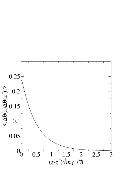
Figure 2: Correlation function of the relative phase fluctuations. The solid line is the numerical calculation of Eq.(49) with $\gamma=g\rho_{0}/10$, $T=\hbar\rho_{0}\sqrt{\gamma}/(2\sqrt{m}k_{B})$ and $L=100\hbar/\sqrt{mg\rho_{0}}$. The dotted line is the analytical expression Eq.(57) which only differs from the numerical expression at small separations.

Figure 3: Phase diagram for the fluctuations of the relative phase between the two condensates. Only temperatures much smaller than $\hbar\rho_{0}\sqrt{g\rho_{0}}/(k_{B}\sqrt{m})$ are relevant as for larger temperatures one does not have a quasi-condensate anymore. For temperatures larger than $\hbar\rho_{0}/(k_{B}L\sqrt{m})$, each condensate has longitudinal phase fluctuations. Below the curve, which corresponds to Eq.(58), the coupling between the condensates is large enough to suppress local relative phase fluctuations between the two condensates. Above this curve, there are local relative phase fluctuations between the two condensates.

IV Dynamical interpretation

The condition (58) to have small relative phase fluctuations has a dynamical interpretation which is shown very qualitatively below. In a two-mode model of the Josephson coupling between two condensates of $N$ atoms it has been shown that if $\gamma\ll N\partial\mu/\partial N$, then the Josephson oscillation frequency is Java99_Josephson ; Stringari2001_Josephson ; Smerzi97_Josephson

$$\omega_{J}=\frac{2}{\hbar}\sqrt{\gamma N\frac{\partial\mu}{\partial N}}\simeq\frac{\sqrt{\gamma\mu}}{\hbar}=\frac{\sqrt{\gamma g\rho_{0}}}{\hbar}.$$ (59)

On the other hand a single elongated condensate will experience phase fluctuations and the phase at a given position will evolve in time. If the change of the phase during a Josephson oscillation time is small, then the Josephson coupling will ensure that the relative phase between the two condensates remains zero: there will be no relative phase fluctuations. However if the change of the phase during a Josephson oscillation time is large, then the Josephson coupling will not have time to adjust the phase of one condensate with respect to the other: there will be relative phase fluctuations of the two condensates. We thus have to compute the change of the local phase of a single condensate

$$\langle(\theta(1/\omega_{J})-\theta(0))^{2}\rangle,$$ (60)

with the average corresponding to the thermal equilibrium and the coupling between the two condensates being ignored. This calculation could be done rigorously by developing the operator $\theta$ on the collective excitation bosonic operators $b_{k}$ and $b_{k}^{{\dagger}}$. In the following we present a simpler argument that gives the same order of magnitude. We first estimate the amplitude $A_{k}$ of the phase modulation of wave vector $k$. The energy of this phase modulation is just the kinetic energy $N|A_{k}|^{2}\hbar^{2}k^{2}/4m$ which in a classical field theory at thermal equilibrium corresponds to an energy of $k_{B}T/2$ and thus

$$|A_{k}|^{2}\simeq\frac{2mk_{B}T}{\hbar^{2}k^{2}}\frac{1}{\rho_{0}L}.$$ (61)

This is indeed the contribution of the mode $k$ to phase fluctuations as computed in Eq.(56) if $\gamma=0$. According to the Bogoliubov spectrum and because only modes with $|k|\ll 2\sqrt{g\rho_{0}m}/\hbar$ contribute, the mode $k$ evolves with the frequency

$$\omega_{k}=\frac{k\sqrt{g\rho_{0}}}{\sqrt{m}}.$$ (62)

The evolution of the phase after a Josephson oscillation time $t_{J}\simeq\hbar/\sqrt{\gamma g\rho_{0}}$ is then written, after averaging over the independent phases of the phase modulations,

$$\langle(\theta(t_{J})-\theta(0))^{2}\rangle \simeq \sum_{k}|A_{k}|^{2}(1-\cos(\omega_{k}t_{J}))$$ (63)

$$\simeq \frac{2mk_{B}T}{\hbar^{2}\rho_{0}2\pi}\int_{-\infty}^{\infty}\frac{1-\cos(\sqrt{t_{J}g\rho_{0}}k/\sqrt{m})}{k^{2}}dk$$

$$\simeq \frac{k_{B}T\sqrt{m}}{\hbar\rho_{0}\sqrt{\gamma}}.$$

Small relative phase fluctuations of the two condensates occurs when this quantity is small and we recover the condition (58).

V discussion

In conclusion we have shown that as long as the temperature is small enough to fulfill Eq.(58), although there might exist large phase fluctuations along each condensate, the local relative phase of the two condensates stays small. In the opposite case there are large fluctuations of the relative phase whose correlation length is $l_{c}=\hbar/2\sqrt{m\gamma}$. As an example let us consider the case of two Rubidium condensates of $10^{4}$ atoms elongated over $L=200\,\mu$m, confined transversely with an oscillation frequency $\omega_{\perp}/2\pi=1\,$kHz and coupled using $\gamma=50\,$Hz. The phase of each condensate changes by about $2\pi$ from one end of the condensate to the other as soon as $T>T_{\phi}=\hbar^{2}\rho_{0}/(mLk_{B})=1.8\,$nK. However the local relative phase between the two condensates stays much smaller than 1 if $T\ll\hbar\rho_{0}\sqrt{\gamma}/(k_{B}\sqrt{m})=180\,$nK. The calculations made here for homogeneous condensates could be used to describe a trapped inhomogeneous gas via a local density approximation similar to that used in Gerbier2002 as long as both the healing length $l_{h}=\hbar/\sqrt{mg\rho_{0}}$ and the correlation length of the phase fluctuations are much smaller than the extension of the condensate. In the above example, $l_{h}=0.6\,\mu$m and $l_{c}=2\,\mu$m are indeed much smaller than $L$.

To measure experimentally the relative phase fluctuations and their correlation length, one should perform an interference experiment. In the case where the two states are internal states, an intense $\pi/2$ pulse has to be applied. Measurement of the local density of atoms in the state $\left|a\right\rangle$ and $\left|b\right\rangle$ then gives access to the local relative phase of the two condensates. In the case where $\left|a\right\rangle$ and $\left|b\right\rangle$ are confined in the wells of a double well potential, the interference measurement is performed via a fast release of the confining potential followed by a time of flight long enough for the two clouds to overlap. Indeed, the total intensity presents fringes in the direction orthogonal to $z$Ketterle-doublepuits and, at a given $z$, the position of the central fringe gives the value of the local relative phase.

References

• (1) S. Dettmer et al., Phys. Rev. Lett. 87, 160406 (2001).
• (2) S. Richard, F. Gerbier, J. H. Thywissen, M. Hugbart, P. Bouyer and A. Aspect, cond-mat/0303137
• (3) M. Girardeau, J. Math. Phys. 1, 516 (1960).
• (4) See D. Petrov, Ph.D. thesis, Amsterdam, 2003, http://www.amolf.nl/publications/theses/petrow and references therein.
• (5) D. Petrov, G. Shlyapnikov, and J. Walraven, Phys. Rev. Lett. 85, 3745 (2000).
• (6) U. A. Khawaja, J. O. Andersen, N. P. Proukakis, and H. T. C. Stoof, Phys.Rev.A 66, 013615 (2002).
• (7) J. O. Andersen, U. A. Khawaja, and H. T. C. Stoof, Phys. Rev. Lett. 88, 070407 (2002).
• (8) C. Mora and Y. Castin, Cond-Mat/0212523 (2002).
• (9) M. R. Matthews, D. S. Hall, D. S. Jin*, J. R. Ensher, C. E. Wieman, and E. A. Cornell, Phys. Rev. Lett. 81, 243 (1998)
• (10) A. Smerzi, S. Fantoni, S. Giovanazzi, and S. R. Shenoy, Phys. Rev. Lett. 79, 4950 (1997).
• (11) J. Javanainen and M. Y. Ivanov, Phys. Rev. A 60, 2351 (1999).
• (12) L. Pitaevskii and S. Stringari, Phys. Rev. Lett. 87, 180402 (2001).
• (13) E. V. Goldstein and P. Meystre, Phys. Rev. A 55, 2935 (1997).
• (14) This approach presents the problem of the definition of the phase operator. For a more rigorous approach, see the work of Popov (V.N. Popov, Functional Integrals in Quantum Field Theory and Statistical physics, D.Reidel Pub., Dordrecht, 1983) or the work of C. Mora and Y. Castin Quasibec_Castin where the space is discretised in cells containing a large number of atoms.
• (15) F. Gerbier et al.,Phys. Rev. A 67, 051602 (2003)
• (16) Y. Shin et al, cond-mat/0306305 (2003)