Magnetic energy-level diagrams of high-spin (Mn₁₂-acetate)
and low-spin (V₁₅) molecules

Abstract

The magnetic energy-level diagrams for models of the Mn₁₂ and V₁₅ molecule are calculated using the Lanczos method with full orthogonalization and a Chebyshev-polynomial-based projector method. The effect of the Dzyaloshinskii-Moriya interaction on the appearance of energy-level repulsions and its relevance to the observation of steps in the time-dependent magnetization data is studied. We assess the usefulness of simplified models for the description of the zero-temperature magnetization dynamics.

I Introduction

Magnetic molecules such as Mn₁₂ or V₁₅ have attracted a lot of interest recently because these nanomagnets can be used to study e.g. quantum (de)coherence, relaxation and tunneling of the magnetization on a nanoscale Gunter ; Caneschi ; gat ; gat2 ; Levine ; Friedman ; Thomas ; sangregorio ; fe8tun ; Bernard ; Perenboom ; Irinel3 ; Pohjola ; Zhong ; Irinel1 ; Irinel5 ; Irinel2 ; Bouk0 ; Bouk1 ; Wernsdorfer ; Honecker ; Irinel4 . As a result of the very weak intramolecular interactions between these molecules, experiments directly probe the magnetization dynamics of the individual molecules. In particular the adiabatic change of the magnetization at low-temperature is governed by the discrete energy-level structure Seiji0 ; Slava0 ; Gunter0 ; Hans2 .

The magnetic properties of molecules such as Mn₁₂ or V₁₅ are often studied by considering a simplified model for the magnetic energy levels for a specific spin multiplet, e.g. S=10 for Mn₁₂ or S=3/2 for V₁₅. However for these and other, similar, magnetic molecules that consist of several magnetic moments (12 in the case of Mn₁₂, 15 in the case of V₁₅), the reduction of the many-body Hamiltonian to an effective Hamiltonian for a specific spin multiplet is, except for the diagonal terms, non-trivial.

Magnetic anisotropy, a result of the geometrical arrangement of the magnetic ions within a molecule of low symmetry, mixes states of different total spin and enforces a treatment of the full Hilbert space of the system. The dominant contribution to the magnetic anisotropy due to spin-orbit interactions is given by the Dzyaloshinskii-Moriya interaction (DMI) Dzy ; Mor ; Kaplan ; Shekntman1 ; Shekntman2 ; Yosida ; Crep . In principle this interaction can change energy-level crossings into energy-level repulsions. The presence of the latter is essential to explain the adiabatic changes of the magnetization at the resonant fields in terms of the Landau-Zener-Stückelberg (LZS) transition Seiji0 ; Slava0 ; Gunter0 ; Hans2 . Thus a minimal magnetic model Hamiltonian should contain (strong) Heisenberg interactions, anisotropic interactions and a coupling to the applied magnetic field Bernard ; Misha1 ; mn12spl ; RudraMn12 ; Rudra ; Seiji1 ; Raghu ; Hans1 ; Konst ; RudraSeiji .

In this paper we calculate the magnetic energy-level diagrams for models of the Mn₁₂ and V₁₅ molecule using exact diagonalization techniques. We study the effect of the DMI on the appearance of energy-level repulsions that determine the adiabatic changes of the magnetization observed experimentally. In contrast to earlier work Rudra ; Konst , the approach adopted in the present paper does not rely on perturbation theory. Instead we perform an exact numerical diagonalization of the full Hamiltonian.

As the quantum spin dynamics of these magnetic molecules is determined by the (tiny) level repulsions, a detailed knowledge of the low-lying energy levels scheme is necessary. In order to bridge the energy scales involved (e.g. from 500K, a typical energy scale for the interaction between individual magnetic ions, to $\approx 10^{-2}-10^{-9}$K, a typical energy scale for energy-level splittings), a calculation of the energy levels of these many-spin Hamiltonians has to be very accurate. We have tested many different standard algorithms to compute the low-lying states. For systems that are too large to be solved by full exact diagonalization, we find that the Lanczos method with full orthogonalization and a Chebyshev-polynomial-based projector method can solve these rather large and difficult eigenvalue problems with sufficient accuracy.

The paper is organized as follows. In Sec. II we introduce the model Hamiltonians for the Mn₁₂ and V₁₅ molecules. In Sec. III we briefly discuss the numerical algorithms that we use to compute the energy levels. Our results for the energy level schemes for Mn₁₂ and V₁₅ are presented in Sec. IV. In Sec. V we analyze a reduced, 3-spin model for V₁₅ and determine the conditions on the DMI energy-level under which repulsions appear. Numerical calculations for the full V₁₅ model confirm that these conditions are also relevant for the presence of energy-level repulsions in the V₁₅ model.

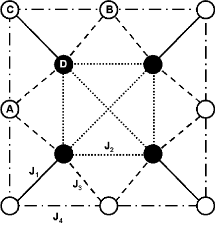
Figure 1: Schematic diagram of the dominant magnetic (Heisenberg) interactions of the Mn₁₂ molecule.

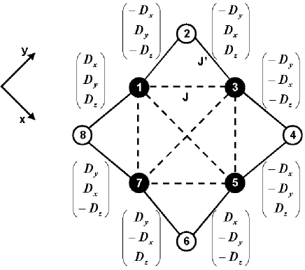
Figure 2: Schematic diagram of the magnetic interactions of the simplified model (1) of the Mn₁₂ molecule.

II Models

II.1 Manganese complex: Mn₁₂

In Fig. 1 we reproduce the schematic diagram of the dominant magnetic (Heisenberg) interactions of the Mn₁₂ molecule (Mn₁₂(CH₃COO)₁₆(H₂O)₄O${}_{12}\cdot$2CH₃COOH$\cdot$4H₂O). The four inner Mn⁺⁴ ions have a spin $S=3/2$, the other eight Mn⁺³ ions have spin $S=2$. The number of different spin states of this system is $4^{4}\times 5^{8}=10^{8}$. If the total magnetization is a conserved quantity, it can be used to block-diagonalize the Hamiltonian, allowing the study of models of this size Raghu ; Regnault . However, to study the adiabatic change of magnetization, we have to treat all the states, and the dimension of the matrix become prohibitively large. Thus we need to simplify the model in order to reduce the dimension. A drastic reduction of the number of spin states can be achieved by assuming that the strong antiferromagnetic Heisenberg interaction ($J_{1}$) between an inner ion and its outer neighbor allows the replacement of the magnetic moment of an inner ion by an effective S=1/2 moment. The schematic diagram of this simplified (but still complicated) model is shown in Fig. 2. The number of different spin states of this model is $2^{4}\times 5^{4}=10^{4}$. In this paper we study the latter model.

The Hamiltonian for the magnetic interactions of the simplified Mn₁₂ model can be written as Misha1

$${\cal H} = -J\Bigl{(}\sum_{i=1}^{4}{\bf S}_{2i-1}\Bigr{)}^{2}-J^{\prime}\sum_{\langle i,j\rangle}{\bf S}_{2i-1}\cdot{\bf S}_{2j}-K_{z}\sum_{i=1}^{4}\left(S_{2i}^{z}\right)^{2}+\sum_{\langle i,j\rangle}{\bf D}^{i,j}\cdot[{\bf S}_{2i-1}\times{\bf S}_{2j}]-\sum_{i=1}^{8}{\bf h}\cdot{\bf S}_{i},$$ (1)

where even (odd) numbered ${\bf S}_{i}$ are the spin operators for the outer (inner) $S=2$ ($S=1/2$) spins. The first two terms describe the isotropic Heisenberg exchange between the spins. The third term describes the single-ion easy-axis anisotropy of $S=2$ spins. In this paper we do not consider higher-order correction terms that restore the SU(2) symmetry Kaplan ; Shekntman1 ; Shekntman2 ; Zheludev . The fourth term represents the antisymmetric DMI in Mn₁₂. The vector ${\bf D}^{i,j}$ determines the DMI between the $i$-th $S=1/2$ spin and the $j$-th $S=2$ spin. The last term describes the interaction of the spins with the external field ${\bf h}$. Note that the factor $g\mu_{B}$ is absorbed in our definition of ${\bf h}$.

The first three terms in Hamiltonian (1) conserve the $z$-component of the total spin $M_{z}=\sum_{i=1}^{8}S^{z}_{i}$. The DMI on the other hand mixes states with different total spin and also states with the same total spin. Hence, the DMI can change level crossings into level repulsions. Therefore, the presence of the DMI may be sufficient to explain the experimentally observed adiabatic changes of the magnetization.

The four-fold rotational-reflection symmetry ($S_{4}$) of the Mn₁₂ molecule imposes some relations between the DM-vectors. It follows that there are only three independent DM-parameters: $D_{x}\equiv D_{x}^{1,8}$, $D_{y}\equiv D_{y}^{1,8}$, and $D_{z}\equiv D_{z}^{1,8}$, as indicated in Fig. 2. The above model satisfactorily describes a rather wide range of experimental data, such as the splitting of the neutron scattering peaks, results of EPR measurements and the temperature dependence of magnetic susceptibility Misha1 . The parameters of this model have been estimated by comparing experimental and theoretical data. In this paper we will use the parameter set B from Ref. Misha1 ; Hans1 : $J=23.8$K, $J^{\prime}=79.2$K, $K_{z}=5.72$K, $D_{x}=22$K, $D_{y}=0$, and $D_{z}=10$K.

Although the amount of available data is not sufficient to fix all these parameters accurately, we expect that the general trends in the energy-level diagram will not change drastically if these parameters change relatively little.

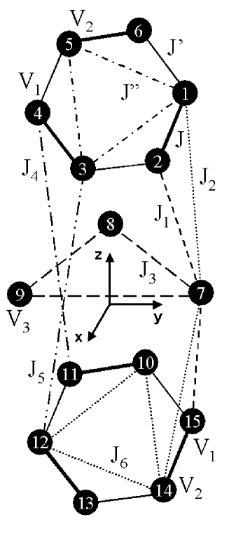
Figure 3: Schematic diagram of the magnetic interactions in model (2) of the V₁₅ molecule.

II.2 Vanadium complex: V₁₅

In Fig. 3 we show the schematic diagram of the dominant magnetic (Heisenberg) interactions of the V₁₅ molecule (K₆[V${}^{IV}_{15}$As₆O₄₂(H₂O)]$\cdot$8H₂O). The magnetic structure consists of two hexagons with six S=1/2 spins each, enclosing a triangle with three S=1/2 spins. All dominant Heisenberg interactions are antiferromagnetic. The number of different spin states of this model is $2^{15}=32768$. The minimal Hamiltonian for the magnetic interactions that incorporates the effects on magnetic anisotropy can be written as Seiji1 ; Rudra ; Konst ; Irinel4

$${\cal H} = -\sum_{\langle i,j\rangle}J_{i,j}{\bf S}_{k}\cdot{\bf S}_{l}+\sum_{\langle i,j\rangle}{\bf D}^{i,j}\cdot[{\bf S}_{i}\times{\bf S}_{j}]-\sum_{i}{\bf h}\cdot S^{z}_{i}.$$ (2)

The various Heisenberg interactions $J_{i,j}$ are shown in Fig. 3. For simplicity, we assume that ${\bf D}^{i,j}=0$ for sites $i$ and $j$ except for bonds for which the Heisenberg exchange constant is $J$ (see Fig. 3) Konst ; Rudra . Rotations about $2\pi/3$ and $4\pi/3$ around the axis perpendicular to and passing through the center of the hexagons leave the V₁₅ complex invariant. This enforces constraints on the values of ${\bf D}^{i,j}$ Konst ; RudraSeiji . In Sec. IV we present results for several different sets of estimates for the model parameters of the V₁₅ model gat2 ; Rudra ; Konst ; Bouk0 .

III Numerical method

A theoretical description of quantum dynamical phenomena in the Mn₁₂ and V₁₅ nanomagnets requires detailed knowledge of their energy-level schemes. Disregarding the fascinating physics of the nanomagnets, the calculation of the eigenvalues of their model Hamiltonians is a challenging problem in its own right. Firstly, the (adiabatic) quantum dynamics of these systems is mainly determined by the (tiny) level repulsions. Therefore the calculation of the energy levels of these many-spin Hamiltonians has to be very accurate in order to bridge the energy scales involved (e.g. from 500K to $\approx 10^{-9}$K). Secondly, the level repulsions originate from the DMI that mix states with different magnetization. In principle, this prevents the use of the magnetization as a vehicle to block-diagonalize the Hamiltonian and effectively reduce the size of the matrices that have to be diagonalized. If a level repulsion involves states of significantly different magnetization (e.g. $M^{z}=-10$ and $M^{z}=10$) a perturbative calculation of the level splitting would require going to rather high order (at least 20), a cumbersome procedure. Therefore it is of interest to explore alternative routes to direct but accurate, brute-force diagonalization of the full model Hamiltonian.

As a non-trivial set of reference data, we used the eigenvalues obtained by full diagonalization (using standard LAPACK algorithms) of the $10000\times 10000$ matrix representing model (1) Hans1 . For one set of model parameters, such a calculation takes about 2 hours of CPU time on an Athlon 1.8 GHz/1.5Gb system. Clearly this is too slow if we want to compute the energy-level diagram as a function of the magnetic field ${\bf h}$. In particular if we want to estimate the structure of the level splittings at the resonant fields we need the eigenvalues for many values of ${\bf h}$. Furthermore, in the case of V₁₅ this calculation would take about 30 times longer and require about 15 Gb of memory which, for present-day computers, is too much to be of practical use.

We have tested different standard algorithms to compute the low-lying eigenvalues of large matrices. The standard Lanczos method (including its conjugate gradient version) as well as the power method WILKINSON ; GOLUB either converge too slowly, lack the accuracy to resolve the (nearly)-degenerate eigenvalues, and sometimes even completely fail to correctly reproduce the low-lying part of the spectrum. This is not a surprise: by construction these methods work well if the ground state is not degenerate and there is little guarantuee that they will work if there are (nearly)-degenerate eigenvalues WILKINSON ; GOLUB . In particular, the Lanczos procedure suffers from numerical instabilities due to the loss of orthogonalization of the Lanczos vectors WILKINSON ; GOLUB . It seems that model Hamiltonians for the nanoscale magnets provide a class of (complex Hermitian) eigenvalue problems that are hard to solve.

Extensive tests lead us to the conclusion that only the Lanczos method with full orthogonalization (LFO) WILKINSON ; GOLUB and a Chebyshev-polynomial-based projector method (CP) (see Appendix) can solve these rather large and difficult eigenvalue problems with sufficient accuracy. The former is significantly faster than the latter but using both gives extra confidence in the results.

In the Lanczos method with full orthogonalization, each time a new Lanczos vector is generated we explicitly orthogonalize (to working precision) this vector to all, not just to the two previous, Lanczos vectors WILKINSON ; GOLUB . With some minor modifications to restart the procedure when the Lanczos iteration terminate prematurely, after $n$ steps this procedure tranforms $n\times n$ matrix $H$ into a tri-diagonal matrix that is comparable in accuracy to the one obtained through Householder tri-diagonalization but offers no advantages GOLUB . In our case we are only interested in a few low-lying eigenstates of $H$. Thus we can exploit the fact that projection onto the (numerically exact) subspace of dimension $k$ ($k\ll n$), built by the Lanczos vectors will yield increasingly accurate estimates of the smallest (largest) eigenvalues and corresponding eigenvectors as $k$ increases.

In practice, to compute the $M$ lowest energy levels, the LFO procedure is carried out as follows.

• Perform a Lanczos step according to the standard procedure

• Use the modified Gramm-Schmidt procedure to orthogonalize the new Lanczos vector with respect to all previous ones WILKINSON ; GOLUB

• Compute the matrix elements of the tridiagonal matrix

• At regular intervals, diagonalize the tridiagonal matrix, compute the approximate eigenvectors $\varphi_{i}$, $\mu_{i}=\langle\varphi_{i}|H|\varphi_{i}\rangle$ and $\Delta^{2}_{i}=\langle\varphi_{i}|(H-\mu_{i})^{2}|\varphi_{i}\rangle$ for $i=1,\ldots,M$, and check if all $\Delta_{i}$ are smaller that a specified threshold. If so, terminate the procedure (the exact eigenvalue $E_{i}$ closest to $\mu_{i}$ satisfies $\mu_{i}-\Delta\leq E_{i}\leq\mu_{i}+\Delta_{i}$). If not, continue generating new Lanczos vectors, etc.

IV Results

IV.1 Manganese complex: Mn₁₂

Figure 4: The lowest 21 energy levels of the Mn₁₂ model (1) as a function of the applied magnetic field ${\bf h}$. Solid lines: eigenstates with $|M^{z}|\approx 10$; dashed lines: eigenstates with $|M^{z}|\approx 9$.

Table 1: The 21 lowest eigenvalues $E_{i}$ and total spin $S_{i}$ of the corresponding eigenstates of the Mn₁₂ model (1) for two values of the external applied field ${\bf h}$ along the $z$-axis. The distance between $E_{i}$ and the exact eigenvalue closest to $E_{i}$ is $\Delta_{i}=\langle\varphi_{i}|(H-E_{i})^{2}|\varphi_{i}\rangle^{1/2}<10^{-10}$ for $i=1,\ldots,7$. These calculations took about 20 minutes on an Athlon 1.8 GHz/1.5Gb system, using 1000 fully orthogonal Lanczos vectors.

$i$	$E_{i}(h=0)$	$S_{i}(h=0)$	$E_{i}(h=5T)$	$S_{i}(h=5T)$
0	-815.1971469173	9.91	-881.7827744750	9.92
1	-815.1971469173	9.91	-860.4928253394	9.93
2	-800.5810020061	9.91	-840.8569089483	9.92
3	-800.5810020061	9.91	-822.8556918884	9.92
4	-787.6124037484	9.91	-815.4339009404	8.93
5	-787.6124037482	9.91	-811.0766283789	8.93
6	-776.2715579413	9.90	-806.4609011890	9.90
7	-776.2715579281	9.90	-797.9409264313	8.94
8	-766.5314713958	9.90	-794.1268159385	8.93
9	-766.5314702412	9.90	-791.6387794071	9.90
10	-758.3618785887	9.89	-781.8373616760	8.93
11	-758.3618126323	9.89	-778.4824830935	8.96
12	-755.6412882369	8.92	-778.3500886860	9.85
13	-755.6412882368	8.92	-776.4751565103	8.93
14	-751.7362729420	9.88	-767.0677893890	8.93
15	-751.7337526641	9.88	-766.5785427469	9.87
16	-751.2349837637	8.91	-764.0838038821	8.92
17	-751.2349837632	8.91	-761.4314952668	8.76
18	-746.6655233754	9.87	-756.2910279030	9.87
19	-746.6082906321	9.87	-753.5740765004	8.92
20	-744.8208087762	8.92	-752.7461619357	8.08

In Table 1 we present the numerical data for $h=0$T and $h=5$T, also obtained by LFO. The results obtained by full exact diagonalization (LAPACK), LFO and CP are the same to working precision (about 13 digits). In Fig. 4 we show the results for the lowest 21 energy levels of the Mn₁₂ model as a function of the applied magnetic field as obtained by LFO.

Although the total magnetization is not a good quantum number, we can label the various eigenstates by their (calculated) magnetization. For large fields and/or energies, eigenstates with total spin 8, 9 and 10 appear, as shown in Table 1. In Fig. 4 eigenstates with $|M^{z}|\approx 10(9)$ (within an error of about 10%) are represented by solid (dashed) lines (eigenstates with $|M^{z}|\approx 8$ appear for $h>4$ but have been omitted for clarity).

The standard $S=10$ single-spin model for Mn₁₂

$${\cal H} = -D(S^{z})^{2}-hS^{z},$$ (3)

is often used as a starting point to interpret experimental results Friedman ; Thomas ; Perenboom ; Irinel3 ; Pohjola ; Rudra . The energy levels of this model exhibit crossings at the resonant fields $h=\pm Dn$ for $n=-10,\ldots,10$, in agreement with our numerical results for the more microscopic model (1). For the parameter set B, we find that $D\approx 0.55K$, in good agreement with experiments Friedman ; Thomas .

The single-spin model (3) commutes with the magnetization $S^{z}$ and therefore it only displays level crossings, no level repulsions. Adding an anisotropy term of the form $S_{+}^{4}+S_{-}^{4}$ only leads to level repulsions when the magnetization changes by 4, which does not agree with the observation of adiabatic changes of the magnetization for all $h=nD$ Friedman ; Thomas ; Perenboom ; Irinel3 . In contrast, for the DMI the Hamiltonian has nonzero matrix elements for the pairs of states $|S,S_{z}\rangle$ and $|S\pm 1,S_{z}\pm 1\rangle$, but zero matrix elements for levels with the same value of the total spin.

In Fig. 4, for some values of $h$, level repulsions are present. However, these are due to the fitting procedure used to plot the data and the number of $h$-values used (100) and disappear by using a higher resolution in ${\bf h}$-fields (results not shown). Thus these splittings have no physical meaning. For the Mn₁₂ system, the energy splittings at low field are extremely small. Their calculation requires extended-precision (128-bit) arithmetic Hans1 . Therefore, to study the structure of the energy-level diagram in more detail we concentrate on the transitions at $h\approx 3.4$T ($M_{z}\approx-10\rightarrow M_{z}\approx 4$)and $h\approx 3.9$T ($M_{z}\approx-10\rightarrow M_{z}\approx 3$) for which adiabatic changes of the magnetization have been observed in experiments Friedman ; Thomas ; Perenboom ; Irinel3 . From experiments one finds that the magnitude of these splittings is of the order of 10 nK private . Extensive calculations lead us to the conclusion that the energy splitting at these resonant fields is smaller than $10^{-6}$K. Adding an extra transverse field by tilting the ${\bf h}$-field by 5 degrees does not change this conclusion. Thus, it is clear that within the (very high) resolution in the ${\bf h}$-field and 13-digit precision of the calculation, there is no compelling evidence that the DMI gives rise to a level repulsion, at least not for the choice of model parameters (set B, see above) considered here. The algorithms developed for the work presented in this paper can be used for 33-digit calculations without modification and we leave the calculation of the splittings for future work.

IV.2 Vanadium complex: V₁₅

Figure 5: Left: The lowest 8 energy levels of V₁₅ model (2) with model parameters taken from Ref. Rudra (VsetA) as a function of the applied magnetic field ${\bf h}$ parallel to the $z$-axis. Right: Detailed view of the four lowest energy levels at $h\approx 0$.

Table 2: The eight lowest eigenvalues $E_{i}$ and total spin $S_{i}$ of the corresponding eigenstates of the V₁₅ model (2) with model parameters taken from Ref. Rudra (VsetA) for two values of the external applied field ${\bf h}$ parallel the $z$-axis. The distance between $E_{i}$ and the exact eigenvalue closest to $E_{i}$ is $\Delta_{i}=\langle\varphi_{i}|(H-E_{i})^{2}|\varphi_{i}\rangle^{1/2}<\times 10^{-9}$ for $i=1,\ldots,7$. These calculations took less than 20 minutes on a Cray SV1 computer, using 521 fully orthogonal Lanczos vectors.

$i$	$E_{i}(h=0)$	$S_{i}(h=0)$	$E_{i}(h=4T)$	$S_{i}(h=4T)$
0	-3679.53623744	0.51	-3683.51181131	1.50
1	-3679.53623744	0.51	-3682.21997451	0.51
2	-3679.52777009	0.51	-3682.18488706	0.53
3	-3679.52777009	0.51	-3678.11784886	1.50
4	-3675.42943612	1.50	-3676.84225573	0.52
5	-3675.42943612	1.50	-3676.83951808	0.51
6	-3675.42325141	1.50	-3672.74011178	1.50
7	-3675.42325141	1.50	-3667.37940477	1.50

For the model parameters given in Ref. Rudra , $J=-800$, $J_{1}=J^{\prime}=-54.4$K, and $J_{2}=J^{\prime\prime}=-160$K, $J_{3}=J_{4}=J_{5}=J_{6}=0$ and in the absence of the DMI, we find for the energy gap between the ground state and the first excited state at $h=0$ a value of 4.12478K, in perfect agreement with Ref. Rudra . Following Ref. RudraSeiji we take for the DMI parameters $D_{x}^{1,2}=D_{y}^{1,2}=D_{z}^{1,2}=40$K, which is approximately 5% of the largest Heisenberg coupling. Using the rotational symmetry of the hexagon we have $D_{x}^{3,4}=14.641$K, $D_{y}^{3,4}=-54.641$K, $D_{z}^{3,4}=40$K and $D_{x}^{5,6}=-54.641$K, $D_{y}^{5,6}=14.641$K, $D_{z}^{5,6}=40$K. As the two hexagons are not equivalent we cannot use symmetry to reduce the number of free parameters. For simplicity, we assume that the $(x,y)$ positions of the spins on the lower hexagons differ from those on the upper hexagon by a rotation about $\pi/3$. This yields for the remaining model parameters $D_{x}^{10,11}=-14.641$K, $D_{y}^{10,11}=54.641$K, $D_{z}^{10,11}=40$K, $D_{x}^{12,13}=-40$K, $D_{y}^{12,13}=-40$K, $D_{z}^{12,13}=40$K, and $D_{x}^{14,15}=54.641$K, $D_{y}^{14,15}=-14.641$K, $D_{z}^{14,15}=40$K. We will refer to this choice as VsetA. In Fig. 5 we show the results for the eight lowest energy levels of V₁₅ model (2) as a function of the applied magnetic field along the $z$-axis, using the parameters VsetA.

From Table 2 we see that for zero field, the DMI splits the doubly-degenerate doublet of $S=1/2$ states into two doublets of $S=1/2$ states. The difference in energy between the doubly-degenerate, first excited states and the two-fold degenerate ground states is due to the DMI and, for the parameters VsetA, has a value of $\approx 0.0085$K, much smaller than the experimental estimate $\approx 0.05$K Irinel4 , but of the same order of magnitude as the values cited in Ref. Konst . The next four higher levels are $S=3/2$ states. The energy-level splitting between the $S=3/2$ and $S=1/2$ states is $\approx 4.1$K, in reasonable agreement with the experimental value $\approx 3.7$K private .

Following Ref. Konst , we take $J=-800$, $J_{1}=J^{\prime}=-225$K, $J_{2}=J^{\prime\prime}=-350$K, and $J_{3}=J_{4}=J_{5}=J_{6}=0$. In the absence of a DMI, we find that the energy gap between the four-fold degenerate ground state and the first excited state is 3.61K, in full agreement with the result of Ref. Konst . Note that this value of the gap is fairly close to the experimental value of 3.7K private . Taking for the non-zero DMIs $D_{x}^{1,2}=D_{x}^{14,15}=25$K, $D_{x}^{3,4}=D_{x}^{5,6}=D_{x}^{10,11}=D_{x}^{12,13}=-12.5$K, $D_{y}^{3,4}=-D_{y}^{5,6}=-D_{y}^{10,11}=D_{y}^{12,13}=-21.5$K, our calculation for the splitting between the two doubly-degenerate S=1/2 levels yields $0.0037$K, about a factor of two larger than the value cited in Ref. Konst . For the energy splitting between the $S=1/2$ and $S=3/2$ levels we obtain $3.616$K instead of the value $3.618$K given in Ref. Konst . These differences seem to suggest that a perturbation approach for the DMI has to be applied with great care kosty . In Fig. 6 we show the results for $J=-800$, $J_{1}=J^{\prime}=-225$K, and $J_{2}=J^{\prime\prime}=-350$K Konst and the same DMI parameters as in VsetA (which we will refer to as VsetB).

For the energy gap at zero field, we find 4.1K and 3.61K for VsetA and VsetB respectively whereas the experimental estimate is 3.7K private . The transition between the states $|1/2,1/2\rangle$ and $|3/2,3/2\rangle$ takes place at $h\approx 2.8$T and $h\approx 3.0$T respectively, also in good agreement with the experimental value $2.8$T.

The most advanced estimation of the model parameters VsetC is given in Ref. Bouk0 . Taking $J=-809$, $J^{\prime}=-120$K, $J^{\prime\prime}=120$K, $J_{1}=-30$K, $J_{2}=-122$K, $J_{3}=-3$K, $J_{4}=-11$K, $J_{5}=-3$K, $J_{6}=-2K$ (see Table I in Ref. Bouk0 ) yields an energy gap of 4.915K, in agreement with Ref. Bouk0 . At $h\approx 3.6$T, the $S=1/2$ and $S=3/2$ states mix, a level repulsion appears and the adiabatic change of the magnetization from $M\approx 1/2$ to $M\approx 3/2$ gives rise to a step in the magnetization versus (time-dependent) ${\bf h}$-field. Although the qualitative features of the energy-level diagram for VsetC also agree with what one would expect on the basis of experiments, the field at which the states $|1/2,1/2\rangle$ and $|3/2,3/2\rangle$ cross, $h\approx 3.6$T, does not compare well to the experimental estimate $h\approx 2.8$T.

On a coarse scale, the level diagrams for VsetA, VsetB and VsetC are all similar and also resemble those of Ref. Konst . However, on a finer $h$-scale a new feature appears (see right panel of Figs. 5, 6, and 7): the field at which the energy difference between the second and third level reaches a minimum is no longer at $h=0$. In other words, in the presence of the DMI, the adiabatic transition between the states $|1/2,-1/2\rangle$ and $|1/2,1/2\rangle$ does not occur. As we show in the next section, this seems to be a generic feature of the DMI in models of V₁₅.

Figure 6: Left: The lowest 8 energy levels of V₁₅ model (2) with model parameters taken from Ref. Konst (VsetB) as a function of the applied magnetic field ${\bf h}$ parallel to the $z$-axis. Right: Detailed view of the four lowest energy levels at $h\approx 0$.

Figure 7: Left: The lowest 8 energy levels of V₁₅ model (2) with model parameters taken from Ref. Bouk0 (VsetC) as a function of the applied magnetic field $h$ parallel the $z$-axis. Right: Detailed view of the four lowest energy levels at $h\approx 0$.

V Discussion

As shown above, the effect of the DMI on the energy-level diagram is much larger for the V₁₅ model than it is for the Mn₁₂ model. Therefore, to study the possibility of using simplified models for capturing the essential time-dependent magnetization dynamics, we will focus on models for the V₁₅ molecule which is somewhat easier to treat numerically. Qualitatively the energy-level scheme for the eight lowest energy levels of the V₁₅ models considered in Sec. IV closely resembles the energy-level diagram of a reduced, anisotropic model of three $S=1/2$ spins described by the Hamiltonian Irinel1 ; Seiji1 ; Konst

$${\cal H} = -J\left({\bf S}_{1}\cdot{\bf S}_{2}+{\bf S}_{2}\cdot{\bf S}_{3}+{\bf S}_{1}\cdot{\bf S}_{3}\right)+{\bf D}^{1,2}\cdot[{\bf S}_{1}\times{\bf S}_{2}]+{\bf D}^{2,3}\cdot[{\bf S}_{2}\times{\bf S}_{3}]+{\bf D}^{1,3}\cdot[{\bf S}_{1}\times{\bf S}_{3}]-\sum_{i=1}^{3}{\bf h}\cdot{\bf S}_{i}.$$ (4)

In the absence of the DMI, fitting the energy-level diagram of model (4) to exprimental data yields $J\approx-2.5$K Irinel1 . We use this estimate to fix $J$ in our numerical calculations. The number of free parameters can be reduced further by exploiting the rotational symmetry of the triangle. We have $D^{1,2}_{x}=D_{x}$, $D^{1,2}_{y}=D_{y}$, $D^{2,3}_{y}=-(\sqrt{3}D_{x}+D_{y})/2$, $D^{1,3}_{x}=-(D_{x}+\sqrt{3}D_{y})/2$, $D^{1,3}_{y}=(\sqrt{3}D_{x}-D_{y})/2$, and $D^{1,2}_{z}=D^{2,3}_{z}=D^{1,3}_{z}=D_{z}$. The numerical results presented in this paper have been obtained for $D_{x}=D_{y}=D_{z}=0.1$K. In Ref. Irinel4 the DMI vector is taken parallel to the $y$-axis at all the bonds and the field is applied along to the $z$-axis. This case corresponds to the case with only $D_{z}$ in the present model with the field applied in the $x$-direction. In this case the gap opens symmetrically with field Irinel4 . However, as we show in this paper, the structure of the gap depends on the direction of the field.

In Fig. 8 we present results for the eight lowest energy levels of the three-spin model (4) as a function of the applied magnetic field along the $z$-axis. Qualitatively it agrees with the level diagram of the full V₁₅ model with parameters VsetA. The effect of the DMI is two-fold: as expected it lifts degeneracies but it may also shift the position of the resonant points in a non-trivial manner. A similar effect was also found in the full model calculations (see Sec. IV).

The butterfly hysteresis loop observed in time-resolved magnetization measurements has been interpreted in terms of combination of a LZS transition at zero field and spin-phonon coupling Irinel1 ; Irinel4 . Here it should be noted that unless the field is applied in a special direction ($x$ or $y$ direction in this case), the set of avoided level crossings is no longer symmetric with respect to the field. Indeed, a closer look at the level diagram (see left picture in Fig. 8) reveals that the mimimum energy difference between the two pairs of levels does not occur at zero field but at $h\approx 0.05$T. This implies that the LZS transition from $|1/2,-1/2\rangle$ to the $|1/2,1/2\rangle$ level does not take place at $h=0$ but at $h\approx 0.05$T. The minimum energy splitting between the first and second level (counting states starting from the ground state) also depends on the direction of the field. For the model parameters used in our calculations, it increases from $0.05$T for ${\bf h}$ parallel to the $z$-axis to $0.12$T for ${\bf h}$ parallel to the $x$-axis (results not shown). The fact that the DMI not only lifts the denegeneracy but, depending on the direction of the field with respect to the symmetry axis, also shifts the resonant point away from $h=0$ seems to be a generic feature.

Summarizing: Our numerical data for the parameters VsetA, VsetB, and VsetC suggest that the three-spin model reproduces the main features of the full V₁₅ model. The presence of the DMI allows for adiabatic changes of the magnetization but, according to our calculations, the value of the resonant field for the $|1/2,-1/2\rangle$ to $|1/2,1/2\rangle$ transition changes with the direction of the magnetic field. This change (by a factor of two at least) should lead to observable changes in the hysteresis loops but has not been seen in experiment private . Therefore, although the DMI causes the avoided level crossing structure, it is anisotropic with respect to the direction of the field. Within the three spin model we have studied the effects of higher-order correction terms that restore the SU(2) symmetry Kaplan ; Shekntman1 ; Shekntman2 ; Zheludev . and found that it has no essential effect on the low energy degenerate doublets while it causes the four $S=3/2$ levels to be degenerate at $h=0$. In experiments only weak directional dependence was found. Thus, another type of mechanism for the gap such as hyper-fine interaction, etc., is necessary and will be studied in the future.

Figure 8: Left: The eight lowest energy levels of V₁₅ model (2) as a function of the applied magnetic field ${\bf h}$ parallel to the $z$-axis. Right: Detailed view of the four lowest energy levels at $h\approx 0$. Note that the energy-level splitting between the second and third level reaches a minimum at $h\approx 0.05$T, not at $h=0$.

Appendix: Projection method

As an alternative to the Lanczos method with full orthogonalization, we have used a power method WILKINSON ; GOLUB based on the matrix exponential $e^{-tH}$ DeRaedt87 . Writing the random vector $\Psi(0)$ in terms of the (unknown) eigenvectors $\{\phi_{i}\}$ of $H$, we find

$$\Psi(t)=e^{-tE_{0}}\left[\phi_{0}\langle\phi_{0}|\Psi(0)\rangle+e^{-t(E_{1}-E_{0})}\phi_{1}\langle\phi_{1}|\Psi(0)\rangle+e^{-t(E_{2}-E_{0})}\phi_{2}\langle\phi_{2}|\Psi(0)\rangle+\ldots\right],$$ (5)

showing $\lim_{t\rightarrow\infty}\Psi(t)/\|\Psi(t)\|\propto\phi_{0}$ if $\langle\phi_{0}|\Psi(0)\rangle\not=0$. In this naive matrix-exponential version of the power method, convergence to the lowest eigenstate is exponential in $t$ if $E_{1}>E_{0}$.

The case of degenerate ($E_{0}=E_{1}=...$) or very close ($E_{0}\approx E_{1}\approx...$) eigenvalues can be solved rather easily by applying the projector to a subspace instead of a single vector, in combination with diagonalization of $e^{tH}$ within this subspace DeRaedt87 . First we fix the dimension $k$ of the subspace by taking $k$ equal or larger than the desired number of distinct eigenvalues. The projection parameter $t$ should be as large as possible but nevertheless sufficiently small so that at least the first $k$ terms survive one projection step. Then we generate a set of random initial vectors $\Psi_{i}(0)$ for $i=1,\ldots,k$ and set the projection count $n$ to zero. We compute the $k$ lowest eigenstates by the following algorithm DeRaedt87

• Perform a projection step $\Psi_{i}((n+1)t)=e^{-tH}\Psi_{i}(nt)$ for $i=1,\ldots,k$.

• Compute the $k\times k$ matrices. $A=\langle\Psi_{i}((n+1)t)|e^{tH}|\Psi_{i}((n+1)t)\rangle=\langle\Psi_{i}((n+1)t)|\Psi_{i}(nt)\rangle$ and $B=\langle\Psi_{i}((n+1)t)|\Psi_{i}(n+1)t)\rangle$. Note that $A$ is hermitian and $B$ is positive definite.

• Determine the unitary transformation $U$ that solves the $k\times k$ generalized eigenvalue problem $Ax=\lambda Bx$. Recall that $k$ is small.

• Compute $\Psi_{i}^{\prime}((n+1)t)=\sum_{j=1}^{k}U_{i,j}\Psi_{j}((n+1)t)$ for $i=1,\ldots,k$.

• Set $\Psi_{i}((n+1)t)=\Psi_{i}^{\prime}((n+1)t)$ for $i=1,\ldots,k$.

• Compute $\mu_{i}=\langle\Psi_{i}((n+1)t)|H|\Psi_{i}((n+1)t)\rangle$ and check if $\Delta^{2}_{i}=\langle\Psi_{i}((n+1)t)|(H-\mu_{i})^{2}|\Psi_{i}((n+1)t)\rangle$ is smaller than a specified threshold for $i=1,\ldots,k$. If yes, terminate the calculation. If no, increase $n$ by one and repeat the procedure.

We calculate $e^{-tH}\Psi$ by using the Chebyshev polynomial expansion method TAL-EZER ; Iitaka01 ; LEFOR ; SILVER ; SlavaCheb . First we compute an upperbound $R$ of the spectral radius of $H$ (i.e., $\|H\|\leq R$) by repeatedly using the triangle inequality SlavaCheb . From this point on we use the “normalized” matrix $\tilde{H}=(2H/R-1)/2$. The eigenvalues of the hermitian matrix $\tilde{H}$ are real and lie in the interval $[-1,1]$ WILKINSON ; GOLUB . Expanding the initial value $\Psi(0)$ in the (unknown) eigenvectors $\phi_{j}$ of $\tilde{H}$ (or $H$) we find

$$\Psi(t)=e^{-tH}\Psi(0)=e^{z\tilde{H}}\Psi(0)=\sum_{j}e^{z\tilde{E}_{j}}\phi_{j}\langle\phi_{j}|\Psi(0)\rangle,$$ (6)

where $z=-tR$. We find the Chebyshev polynomial expansion of $\Psi(t)$ by computing the Fourier coefficients of the function $e^{z\cos\theta}$ ABRAMOWITZ . Alternatively, since $-1\leq\tilde{E}_{j}\leq 1$, we can use the expansion $e^{z\tilde{E}_{j}}=I_{0}(z)+2\sum_{m=1}^{\infty}I_{m}(z)T_{m}(\tilde{E}_{j})$ where $I_{m}(z)$ is the modified Bessel function of integer order $m$ ABRAMOWITZ to write Eq. (6) as

$$\Psi(t)=\left[I_{0}(z)I+2\sum_{m=1}^{\infty}I_{m}(z)T_{m}(\tilde{H})\right]\Psi(0)\,.$$ (7)

Here, $I$ is the identity matrix and $T_{m}(\tilde{H})$ is the matrix-valued Chebyshev polynomial defined by the recursion relations

$$T_{0}(\tilde{H})\Psi(0)=\Psi(0)\,,\quad T_{1}(\tilde{H})\Psi(0)=\tilde{H}\Psi(0)\,,$$ (8)

and

$$T_{m+1}(\tilde{H})\Psi(0)=2\tilde{H}T_{m}(\tilde{H})\Psi(0)-T_{m-1}(\tilde{H})\Psi(0)\,,$$ (9)

for $m\geq 1$. In practice we will sum only contributions with $m\leq M$ where $M$ is choosen such that for all $m>M$, $|I_{m}(z)/I_{0}(z)|$ is zero to machine precision. Then it is not difficult to show that $\|e^{-tH}/I_{0}(z)-I-2\sum_{m=1}^{M}[I_{m}(z)/I_{0}(z)]T_{m}(\tilde{H})\|$ is zero to machine precision too (instead of $e^{-tH}$ we can equally well use $e^{-tH}/I_{0}(z)$ as the projector).

Using the downward recursion relation of the modified Bessel functions, we can compute $K$ Bessel functions to machine precision using only of the order of $K$ arithmetic operations ABRAMOWITZ ; NumericalRecipes . A calculation of the first 20000 modified Bessel functions takes less than 1 second on a Pentium III 600 MHz mobile processor, using 14-15 digit arithmetic. Hence this part of a calculation is a negligible fraction of the total computational work for solving the eigenvalue problem. Performing one projection step with $e^{-tH}$ amounts to repeatedly using recursion (9) to obtain $\widetilde{T}_{m}(B)\Psi(0)$ for $k=2,\ldots,M$, multiply the elements of this vector by $I_{m}(z)$ and add all contributions.

References

- (1) Quantum Tunneling of Magnetization, eds. L. Gunther and B. Barbara, NATO ASI Ser. E, Vol. 301 (Kluwer, Dordrecht, 1995).
- (2) A. Caneschi, D. Gatteschi, R. Sessoli, A. Barra, L.C. Brunel, and M. Guillot, J. Am. Chem. Soc. 113, 5873 (1991).
- (3) R. Sessoli, H.-L. Tsai, A. R. Shake, S. Wang, J. B. Vincent, K. Folting, D. Gatteschi, G. Christou, D. N. Hendrickson, J. Am. Chem. Soc. 115, 1804 (1993).
- (4) D. Gatteschi, L. Pardi, A.L. Barra, and A. Müller, Mol. Eng. 3, 157 (1991).
- (5) G. Levine and J. Howard, Phys. Rev. Lett. 75, 4142 (1995).
- (6) J.R. Friedman, M.P. Sarachik, J. Tejada, and R. Ziolo, Phys. Rev. Lett. 76, 3830 (1996).
- (7) L. Thomas, F. Lionti, R. Ballou, D. Gattesehi, R. Sessoli, and B. Barbara, Nature 383, 145 (1996).
- (8) C. Sangregorio, T. Ohm, C. Paulsen, R. Sessoli, D. Gatteschi, Phys. Rev. Lett. 78, 4645 (1997).
- (9) W. Wernsdorfer and R. Sessoli, Science 284, 133 (1999); W. Wernsdorfer, T. Ohm, C. Sangregorio, R. Sessoli, D. Mailly, and C.Paulsen, Phys. Rev. Lett. 82, 3903 (1999).
- (10) B. Barbara, L. Thomas, F. Lionti, A. Sulpice, and A. Caneschi, J. Magn. Magn. Mater. 177, 1324 (1998).
- (11) J.A.A.J. Perenboom, J.S. Brooks, S. Hill, T. Hathaway, and N.S. Dalal, Phys. Rev B 58, 330 (1998).
- (12) I. Chiorescu, W. Wernsdorfer, A. Müller, H. Bögge, and B. Barbara, Phys. Rev. Lett. 84, 3454 (2000).
- (13) T. Pohjola and H. Schoeller, Phys. Rev. B 62, 15026 (2000).
- (14) Y. Zhong, M.P. Sarachik, J. Yoo, and D.N. Hendrickson, Phys. Rev. B 62, R9256 (2000).
- (15) I. Chiorescu, W. Wernsdorfer, A. Müller, H. Bögge, and B. Barbara, J. Magn. Magn. Mater. 221, 103 (2000).
- (16) I. Chiorescu, W. Wernsdorfer, A. Müller, H. Bögge, and B. Barbara, Phys. Rev. Lett. 84, 3454 (2000).
- (17) I. Chiorescu, R. Giraud, A.G.M. Jansen, A. Caneschi, and B. Barbara, Phys. Rev. Lett. 85, 4807 (2000).
- (18) D.W. Boukhvalov, V.V. Dobrovitski, M.I. Katsnelson, A.I. Lichtenstein, B.N. Harmon, and P. Kögerler, J. Appl. Phys. 93, 7082 (2003).
- (19) D.W. Boukhvalov, A.I. Lichtenstein, V.V. Dobrovitski, M.I. Katsnelson, B.N. Harmon, V.V. Mazurenko, and V.I. Anisimov, arXiv:cond-mat/0110488.
- (20) W. Wernsdorfer, N. Allaga-Alcalde, D.N. Hendrickson, and G. Christou, Nature 416, 407 (2002).
- (21) A. Honecker, F. Meier, D. Loss, and B. Normand, Eur. Phys. J. B 27, 487 (2002).
- (22) I. Chiorescu, W. Wernsdorfer, A. Müller, S. Miyashita, and B. Barbara, arXiv: cond-mat/0212181.
- (23) S. Miyashita, J. Phys. Soc. Jpn. 64, 3207 (1997); ibid. 65 2734 (1996).
- (24) V.V. Dobrovitskii and A.K. Zvezdin, Europhys. Lett. 38, 377 (1997).
- (25) L. Gunther, Europhys. Lett. 39, 1 (1997).
- (26) H. De Raedt, S. Miyashita, K. Saitoh, D. García-Pablos and N. García, Phys. Rev. B 56, 11761 (1997).
- (27) I.E. Dzyaloshinskii, Zh. Eksp. Teor. Fiz. 32, 1547 (1957), [Sov. Phys. JETP 5, 1259 (1957)].
- (28) T. Moriya, Phys. Rev. 120, 91 (1960).
- (29) T.A. Kaplan, Z. Phys. B 49, 313 (1983).
- (30) L. Shekhtman, O. Entin-Wohlman, and A. Aharony, Phys. Rev. Lett. 69, 836 (1992).
- (31) L. Shekhtman, A. Aharony, and O. Entin-Wohlman, Phys. Rev. B. 47, 174 (1993).
- (32) K. Yosida, Theory of Magnetism, (Springer-Verlag, Berlin, New York, 1996).
- (33) A. Crépieux and C. Lacroix, J. Magn. Magn. Mater. 182, 341 (1998).
- (34) M.I. Katsnelson, V.V. Dobrovitski, and B.N. Harmon, Phys. Rev. B 59, 6919 (1999).
- (35) M. Al-Saqer, V. V. Dobrovitski, B. N. Harmon, and M. I. Katsnelson, J. Appl. Phys. 87, 6268 (2000).
- (36) I. Rudra, S. Ramasesha, and D. Sen, Phys. Rev. B 64, 014408 (2001).
- (37) I. Rudra, S. Ramasesha, and D. Sen, J. Phys.: Condens. Matter 13, 11717 (2001).
- (38) S. Miyashita and N. Nagaosa, Prog. Theor. Phys. 106, 533 (2001).
- (39) C. Raghu, I. Rudra, D. Sen, and S. Ramasesha, Phys. Rev. B 64, 064419 (2001).
- (40) H. De Raedt, A.H. Hams, V.V. Dobrovitsky, M. Al-Saqer, M.I. Katsnelson, and B.N. Harmon, J. Magn. Magn. Mat. 246, 392 (2002).
- (41) N.P. Konstantinidis and D. Coffey, Phys. Rev. B 66, 174426 (2002).
- (42) I. Rudra, K. Saitoh, S. Ramasesha, and S. Miyashita, subm. to J. Phys. Soc. Jpn.
- (43) N. Regnault, Th. Jolicoeur, R. Sessoli, D. Gatteschi, and M. Verdaguer, Phys. Rev. B 66, 054409 (2002).
- (44) A. Zheludev, S. Maslov, I. Tsukada, I. Zaliznyak, L. P. Regnault, T. Masuda, K. Uchinokura, R. Erwin, and G. Shirane, Phys. Rev. Lett. 81, 5410 (1998).
- (45) I. Chiorescu, private communication
- (46) V.V. Kostyuchenko and A.K. Zvezdin, Phys. Solid State 45, 903 (2003).
- (47) J.H. Wilkinson, The Algebraic Eigenvalue Problem, (Clarendon Press, Oxford, 1965).
- (48) G.H. Golub and C.F. Van Loan, Matrix Computations, (John Hopkins University Press, Baltimore, 1996).
- (49) H. De Raedt, Comp. Phys. Rep. 7, 1 (1987).
- (50) H. Tal-Ezer and R. Kosloff, J. Chem. Phys. 81, 3967 (1984).
- (51) C. Leforestier, R.H. Bisseling, C. Cerjan, M.D. Feit, R. Friesner, A. Guldberg, A. Hammerich, G. Jolicard, W. Karrlein, H.-D. Meyer, N. Lipkin, O. Roncero, and R. Kosloff, J. Comp. Phys. 94, 59 (1991).
- (52) T. Iitaka, S. Nomura, H. Hirayama, X. Zhao, Y. Aoyagi, and T. Sugano, Phys. Rev. E 56, 1222 (1997).
- (53) R.N. Silver and H. Röder, Phys. Rev. E 56, 4822 (1997).
- (54) V.V. Dobrovitski and H.A. De Raedt, Phys. Rev. E 67, 056702 (2003).
- (55) M. Abramowitz and I. Stegun, Handbook of Mathematical Functions, (Dover, New York, 1964).
- (56) W.H. Press, B.P. Flannery, S.A. Teukolsky, and W.T. Vetterling, Numerical Recipes, (Cambridge, New York, 1986).