The critical behavior of magnetic systems described by Landau-Ginzburg-Wilson field theories

Pasquale Calabrese,^a Andrea Pelissetto,^b Ettore Vicari${}^{c\;*}$

^a Scuola Normale Superiore, Pisa, Italy

^b Dipartimento di Fisica dell’Università di Roma I, Roma, Italy

^c Dipartimento di Fisica dell’Università di Pisa, Pisa, Italy

E-mail: calabres@df.unipi.it, Andrea.Pelissetto@roma1.infn.it,

Ettore.Vicari@df.unipi.it

We discuss the critical behavior of several three-dimensional magnetic systems, such as pure and randomly dilute (anti)ferromagnets and stacked triangular antiferromagnets. We also discuss the nature of the multicritical points that arise in the presence of two distinct $O(n)$-symmetric order parameters and, in particular, the nature of the multicritical point in the phase diagram of high-$T_{c}$ superconductors that has been predicted by the SO(5) theory. For each system, we consider the corresponding Landau-Ginzburg-Wilson field theory and review the field-theoretical results obtained from the analysis of high-order perturbative series in the frameworks of the $\epsilon$ and of the fixed-dimension $d=3$ expansions.

1 Introduction

In the framework of the renormalization-group (RG) approach to critical phenomena, a quantitative description of many continuous phase transitions can be obtained by considering an effective Landau-Ginzburg-Wilson (LGW) theory, containing up to fourth-order powers of the field components. The simplest example is the O($N$)-symmetric $\phi^{4}$ theory,

$${\cal H}_{O(N)}=\int d^{d}x\Bigl{[}{1\over 2}\sum_{i}(\partial_{\mu}\Phi_{i})^{2}+{1\over 2}r\sum_{i}\Phi_{i}^{2}+{1\over 4!}u\sum_{ij}\Phi_{i}^{2}\Phi_{j}^{2}\Bigr{]},$$ (1)

where $\Phi$ is an $N$-component real field. This model describes several universality classes: the Ising one for $N=1$ (relevant for the liquid-vapor transition in simple fluids, for the Curie transition in uniaxial magnetic systems, etc…), the XY one for $N=2$ (relevant for the superfluid transition in ⁴He, and the magnetic transition in magnets with easy-plane anisotropy, etc…), the Heisenberg one for $N=3$ (it describes the Curie transition in isotropic magnets), the O(4) universality class for $N=4$ (relevant for the finite-temperature transition in two-flavor quantum chromodynamics, the theory of strong interactions); in the limit $N\rightarrow 0$ it describes the behavior of dilute homopolymers in a good solvent in the limit of large polymerization. See, e.g., Refs. [1, 2] for recent reviews. But there are also other physically interesting transitions described by LGW field theories characterized by more complex symmetries.

The general LGW Hamiltonian for an $N$-component field $\Phi_{i}$ can be written as

$${\cal H}=\int d^{d}x\Bigl{[}{1\over 2}\sum_{i}(\partial_{\mu}\Phi_{i})^{2}+{1\over 2}\sum_{i}r_{i}\Phi_{i}^{2}+{1\over 4!}\sum_{ijkl}u_{ijkl}\;\Phi_{i}\Phi_{j}\Phi_{k}\Phi_{l}\Bigr{]},$$ (2)

where the number of independent parameters $r_{i}$ and $u_{ijkl}$ depends on the symmetry group of the theory. An interesting class of models are those in which $\sum_{i}\Phi^{2}_{i}$ is the only quadratic invariant polynomial. In this case, all $r_{i}$ are equal, $r_{i}=r$, and $u_{ijkl}$ satisfies the trace condition [3]

$$\sum_{i}u_{iikl}\propto\delta_{kl}.$$ (3)

In these models, criticality is driven by tuning the single parameter $r$. Therefore, they describe critical phenomena characterized by one (parity-symmetric) relevant parameter, which often corresponds to the temperature. Of course, there is also (at least one) parity-odd relevant parameter that corresponds to a term $\sum_{i}h_{i}\Phi_{i}$ that can be added to the Hamiltonian (2). For symmetry reasons, criticality occurs for $h_{i}\to 0$. There are several physical systems whose critical behavior can be described by this type of LGW Hamiltonians with two or more quartic couplings, see, e.g., Refs. [4, 2]. More general LGW Hamiltonians, that allow for the presence of independent quadratic parameters $r_{i}$, must be considered to describe multicritical behaviors arising from the competition of distinct types of ordering. A multicritical point can be observed at the intersection of two critical lines with different order parameters. In this case the multicritical behavior is achieved by tuning two relevant scaling fields, which may correspond to the temperature and to an anisotropy parameter [5].

In the field-theoretical (FT) approach the RG flow is determined by a set of RG equations for the correlation functions of the order parameter. In the case of a continuous transition, the critical behavior is determined by the stable fixed point (FP) of the theory, which characterizes a universality class. The absence of a stable FP may instead be considered as an indication for a first-order transition, even in those cases in which the mean-field approximation predicts a continuous transition. But, even in the presence of a stable FP, a first-order transition may still occur for systems that are outside its attraction domain. The RG flow can be studied by perturbative methods, by performing an expansion in powers of $\epsilon\equiv 4-d$ [6] or a fixed-dimension (FD) expansion in powers of appropriate zero-momentum quartic couplings [7]. It is also possible to combine the FD approach with the $4-d$ regularization, obtaining the minimal-subtraction scheme without $\epsilon$ expansion [8]. In these perturbative approaches, the computation and the resummation of high-order series is essential to obtain reliable results for three-dimensional transitions (see Refs. [1, 2] for reviews). Beside improving the accuracy, in some cases high-order calculations turn out to be necessary to determine the correct physical picture in three dimensions.

In this paper we discuss the applications of the FT approach to the study of several three-dimensional transitions in magnetic systems. Beside the O($N$)-symmetric Hamiltonian ${\cal H}_{O(N)}$ that is relevant for magnetic transition in uniaxial, easy-plane, and isotropic magnets, we consider LGW Hamiltonians characterized by more complex symmetries: in particular, we consider Hamiltonians invariant under the cubic group, under O($M$)$\otimes$O($N$) and O($M$)$\oplus$O($N$). They allow us to investigate the effects of the addition of uncorrelated nonmagnetic impurities to magnetic systems, the critical behavior of frustrated spin models with noncollinear order—we can check whether a new chiral universality class exists—and the nature of the multicritical points arising from the competition of distinct $O(n)$ order parameters. We present an overview of results obtained by using perturbative FT methods and compare them with other theoretical approaches that provide results of comparable precision—first of all, with results obtained using lattice techniques, e.g., Monte Carlo and high-temperature expansions—and with experiments.

The paper is organized as follows. Sec. 2 is dedicated to the standard O($N$) universality classes. We present a brief overview of FT results for the universality classes that are relevant for magnetic systems, such as the Ising, XY, and Heisenberg ones. In Sec. 3 we analyze the stability of the O($N$)-symmetric FP under generic perturbations in three-dimensional $N$-component systems. This analysis is useful to assess the relevance of magnetic anisotropies in the critical behavior of physical systems. In Sec. 4 we discuss the effects of the addition of quenched nonmagnetic impurities on the critical behavior of magnetic systems, focusing on pure systems that have transitions belonging to the standard O($N$) universality classes. In Sec. 5 we consider frustrated spin models with noncollinear order, whose critical behavior is effectively described by an O($M$)$\otimes$O($N$)-symmetric Hamiltonian with $M=2$. These models are relevant for stacked triangular antiferromagnets. In Sec. 6 we consider the O($n_{1}$)$\oplus$O($n_{2}$)-symmetric $\phi^{4}$ theory that describes the universal behavior near the multicritical point where two critical lines with symmetry O($n_{1}$) and O($n_{2}$) meet. Finally, we discuss the relevance of these results for anisotropic antiferromagnets in the presence of a magnetic field and for high-$T_{c}$ superconductors within the so-called SO(5) theory.

2 The O($N$) universality classes

The O($N$) universality classes are relevant for magnetic systems, because they describe the critical behaviors in uniaxial, easy-plane, and isotropic magnets, corresponding respectively to the Ising ($N=1$), XY ($N=2$) and Heisenberg ($N=3$) universality classes. The universal critical properties can be investigated by using perturbative FT methods applied to the O($N$)-symmetric Hamiltonian (1). The oldest perturbative method is the $\epsilon$ expansion in which the expansion parameter is $\epsilon\equiv 4-d$ [6]. Subsequently, Parisi [7] pointed out the possibility of using pertubation theory directly at the physical dimensions $d=3$ and $d=2$ in the massive (high-temperature) phase.

2.1 The fixed-dimension expansion

In the FD expansion one works directly in $d=3$ or $d=2$. In this case the theory is super-renormalizable since the number of primitively divergent diagrams is finite. One may regularize the corresponding integrals by keeping $d$ arbitrary and performing an expansion in $\epsilon=3-d$ or $\epsilon=2-d$. Poles in $\epsilon$ appear in divergent diagrams. Such divergences are related to the necessity of performing an infinite renormalization of the parameter $r$ appearing in the bare Hamiltonian, see, e.g., the discussion in Ref. [9]. This problem can be avoided by replacing the quadratic parameter $r$ of the Hamiltonian with the mass $m$ (inverse second-moment correlation length) defined by

$$m^{-2}=\,{1\over\Gamma^{(2)}(0)}\,\left.{\partial\Gamma^{(2)}(p^{2})\over\partial p^{2}}\right|_{p^{2}=0},$$ (4)

where the function $\Gamma^{(2)}(p^{2})$ is related to the one-particle irreducible two-point function (i.e. the inverse two-point function of the order-parameter field) by

$$\Gamma^{(2)}_{ab}(p)=\delta_{ab}\Gamma^{(2)}(p^{2}).$$ (5)

Perturbation theory in terms of $m$ and $u$ is finite in $d<4$. The critical limit is obtained for $m\to 0$. To handle it, one considers appropriate RG functions. Specifically, one defines the zero-momentum four-point coupling $g$ and the field-renormalization constant $Z_{\phi}$ by

$$\Gamma^{(2)}_{ab}(p)=\delta_{ab}Z_{\phi}^{-1}\left[m^{2}+p^{2}+O(p^{4})\right],$$ (6)

$$\Gamma^{(4)}_{abcd}(0)=Z_{\phi}^{-2}m^{4-d}{g\over 3}\left(\delta_{ab}\delta_{cd}+\delta_{ac}\delta_{bd}+\delta_{ad}\delta_{bc}\right),$$ (7)

where $\Gamma^{(n)}_{a_{1},\ldots,a_{n}}$ are one-particle irreducible correlation functions. Then, one defines a coupling-renormalization constant $Z_{g}$ and a mass-renormalization constant $Z_{t}$ by

$$u=m^{4-d}gZ_{g}Z_{\phi}^{-2},\qquad\Gamma^{(1,2)}_{ab}(0)=\,\delta_{ab}Z_{t}^{-1},$$ (8)

where $\Gamma^{(1,2)}_{ab}(p)$ is the one-particle irreducible two-point function with an insertion of ${1\over 2}\phi^{2}$. The renormalization constants are determined as perturbative expansions in powers of $g$. The FP of the model is determined by the nontrivial zero $g^{*}$ of the $\beta$-function

$$\beta(g)=m\left.{\partial g\over\partial m}\right|_{u}=(d-4)g\left[1+g{d\over dg}\log(Z_{g}Z_{\phi}^{-2})\right]^{-1}.$$ (9)

Then, one defines

$$\eta_{\phi}(g)=\left.{\partial\ln Z_{\phi}\over\partial\ln m}\right|_{u}=\beta(g){\partial\ln Z_{\phi}\over\partial g},$$ (10)

$$\eta_{t}(g)=\left.{\partial\ln Z_{t}\over\partial\ln m}\right|_{u}=\beta(g){\partial\ln Z_{t}\over\partial g}.$$ (11)

Finally, the critical exponents are given by

$$\eta = \eta_{\phi}(g^{*}),$$ (12)

$$\nu = \left[2-\eta_{\phi}(g^{*})+\eta_{t}(g^{*})\right]^{-1},$$ (13)

$$\omega = \beta^{\prime}(g^{*}),$$ (14)

where $\omega$ is the exponent associated with the leading irrelevant operator. All other exponents can be obtained using the scaling and hyperscaling relations.

In three dimensions the $\beta$-function is known to six loops [10], while the RG functions associated with the critical exponents have been computed to seven loops [11]. FT perturbative expansions are divergent. Thus, in order to obtain accurate results, an appropriate resummation is required. This can be done by exploiting their Borel summability, and the knowledge of the high-order behavior of the expansion, see, e.g., Ref. [12]. In Table 1 we report some recent results for the critical exponents of the Ising, XY, and Heisenberg universality classes. For comparison, we also report estimates from lattice techniques, such as high-temperature (HT) expansions and Monte Carlo (MC) simulations. The agreement is very good. A much more complete list of results and references can be found in Ref. [2]. Of course, it is important to note that there is also a good general agreement with experiments, see, e.g., the list of results reported in Ref. [2].

Since this FD expansion is based on zero-momentum renormalization conditions, it is not suited for the study of the low-temperature (broken) phase. In order to investigate the low-temperature phase other perturbative FD schemes should be considered, such as the minimal-subtraction scheme without $\epsilon$ expansion [8].

2.2 The $\epsilon$ expansion

The $\epsilon$ expansion [6] is based on the observation that, for $d=4$, the theory is essentially Gaussian. One considers the standard perturbative expansion, and then transforms it into an expansion in powers of $\epsilon\equiv 4-d$. In practice, the method works as in the FD expansion. One first determines the expansion of the renormalization constants $Z_{g}$, $Z_{\phi}$, and $Z_{t}$ in powers of the coupling $g$. Initially, they were obtained by requiring the normalization conditions (6), (7), and (8). However, in this framework it is simpler to use the minimal-subtraction scheme [18]. Once the renormalization constants are determined, one computes the RG functions $\beta(g)$, $\eta_{\phi}(g)$, and $\eta_{t}(g)$ as in Sec. 2.1. The FP value $g^{*}$ is obtained by solving the equation $\beta(g^{*})=0$ perturbatively in $\epsilon$. Once the expansion of $g^{*}$ is available, one obtains the expansion of the exponents, by expressing $\eta_{\phi}(g^{*})$ and $\eta_{t}(g^{*})$ in powers of $\epsilon$. In this scheme, five-loop series for the exponents were computed in Refs. [19, 20]. The results of their analysis, exploiting Borel summability, are reported in Table 1. Again the results are in good agreement with the other approaches.

Table 1: Three-dimensional estimates of the critical exponents from the analysis of the fixed-dimension (FD) and $\epsilon$ expansions, and from lattice techniques such as high-temperature (HT) expansions and Monte Carlo simulations.

$N$		$\nu$	$\eta$	$\alpha$	$\gamma$	$\beta$
1	FD exp [13]	0.6303(8)	0.0335(25)	0.1091(24)	1.2396(13)	0.3258(14)
	$\epsilon$ exp [13]	0.6305(25)	0.0365(50)	0.108(7)	1.2380(50)	0.3265(15)
	HT exp [14]	0.63012(16)	0.03639(15)	0.1096(5)	1.2373(2)	0.32653(10)
	MC [15]	0.6297(5)	0.0362(8)	0.1109(15)	1.2366(15)	0.3262(4)
2	FD exp [13]	0.6703(15)	0.0354(25)	$-$0.011(4)	1.3169(20)	0.3470(11)
	$\epsilon$ exp [13]	0.6680(35)	0.0380(50)	$-$0.004(11)	1.3110(70)	0.3467(25)
	HT exp [16]	0.67155(27)	0.0380(4)	$-$0.0146(8)	1.3177(5)	0.3485(2)
	MC [16]	0.6716(5)	0.0380(5)	$-$0.0148(15)	1.3177(10)	0.3486(3)
3	FD exp [13]	0.7073(35)	0.0355(25)	$-$0.122(10)	1.3895(50)	0.3662(25)
	$\epsilon$ exp [13]	0.7045(55)	0.0375(45)	$-$0.114(16)	1.382(9)	0.3655(50)
	HT exp [17]	0.7112(5)	0.0375(5)	$-$0.1336(15)	1.3960(9)	0.3689(3)
	MC [17]	0.7113(11)	0.0378(6)	$-$0.1339(33)	1.3957(22)	0.3691(6)

3 Stability of the O($N$)-symmetric fixed point in 3-D multicomponent systems

In order to discuss the stability of the O($N$) FP in a generic $N$-component system, we consider the general problem of an O($N$)-symmetric Hamiltonian in the presence of a perturbation $P$, i.e.,

$${\cal H}=\int d^{d}x\left[{\textstyle\frac{1}{2}}(\partial_{\mu}\Phi)^{2}+{\textstyle\frac{1}{2}}r\Phi^{2}+{\textstyle\frac{1}{4!}}u(\Phi^{2})^{2}+h_{p}P\right],$$ (15)

where $\Phi$ is an $N$-component field and $h_{p}$ an external field coupled to $P$. Assuming $P$ to be an eigenoperator of the RG transformations, the singular part of the Gibbs free energy for the reduced temperature $t\to 0$ and $h_{p}\to 0$ can be written as

$${\cal F}_{\rm sing}(t,h_{p})\approx|t|^{d\nu}\widehat{\cal F}\left(h_{p}|t|^{-\phi_{p}}\right),$$ (16)

where $\phi_{p}\equiv y_{p}\nu$ is the crossover exponent associated with the perturbation $P$, $y_{p}$ is the RG dimension of $P$, and $\widehat{\cal F}(x)$ is a scaling function. If $y_{p}>0$ the pertubation is relevant and its presence causes a crossover to another critical behavior or to a first-order transition.

In order to discuss the stability of the O($N$) FP in general, we must consider any perturbation of the O($N$) FP. We shall first consider perturbations that are polynomials of the field $\Phi^{a}$. Any such perturbation can be written [21] as a sum of terms $P_{k,l}^{a_{1},\ldots,a_{l}}$, $k\geq l$, which are homogeneous in $\Phi^{a}$ of degree $k$ and transform as the $l$-spin representation of the O($N$) group. Explicitly, we have

$$P_{k,{l}}^{a_{1},\ldots,a_{l}}=(\Phi^{2})^{(k-l)/2}Q_{l}^{a_{1},\ldots,a_{l}}$$ (17)

where $Q_{l}^{a_{1},\ldots,a_{l}}$ is a homogeneous polynomial of degree $l$ that is symmetric and traceless in the $l$ indices. The lowest-order polynomials are

$$Q_{1}^{a}=\Phi^{a},$$ (18)

$$Q^{ab}_{2}=\Phi^{a}\Phi^{b}-{1\over N}\delta^{ab}\Phi^{2}$$ (19)

$$Q_{3}^{abc}=\Phi^{a}\Phi^{b}\Phi^{c}-{1\over N+2}\Phi^{2}\left(\Phi^{a}\delta^{bc}+\Phi^{b}\delta^{ac}+\Phi^{c}\delta^{ab}\right),$$ (20)

$$Q^{abcd}_{4}=\Phi^{a}\Phi^{b}\Phi^{c}\Phi^{d}$$

$$\;-{1\over N+4}\Phi^{2}\left(\delta^{ab}\Phi^{c}\Phi^{d}+\delta^{ac}\Phi^{b}\Phi^{d}+\delta^{ad}\Phi^{b}\Phi^{c}+\delta^{bc}\Phi^{a}\Phi^{d}+\delta^{bd}\Phi^{a}\Phi^{c}+\delta^{cd}\Phi^{a}\Phi^{b}\right)$$

$$\;+{1\over(N+2)(N+4)}(\Phi^{2})^{2}\left(\delta^{ab}\delta^{cd}+\delta^{ac}\delta^{bd}+\delta^{ad}\delta^{bc}\right).$$ (21)

The classification in terms of spin values is particularly convenient, since polynomials with different spin do not mix under RG transformations. On the other hand, operators with different $k$ but with the same $l$ do mix under renormalization. At least near four dimensions, we can use standard power counting to verify that the perturbation with indices $m,l$ mixes only with $P_{k^{\prime},l}$, $k^{\prime}\leq k$. In particular, $P_{l,l}$ renormalizes multiplicatively and is therefore a RG eigenoperator. Moreover, if $y_{k,l}$ is the RG dimension of the appropriately subtracted $P_{k,l}$, one can verify that for small $\epsilon$, $y_{k,l}<0$, for $l\geq 5$, i.e. the only relevant operators have $l\leq 4$. It is reasonable to assume that this property holds up to $\epsilon=1$. In principle, one should also consider terms with derivatives of the field, but again one can show that they are all irrelevant or redundant. Note that the condition that $\sum\Phi^{2}_{i}$ is the only quadratic invariant of the theory forbids the presence in the Hamiltonian of any spin-2 term $P^{ab}_{2,2}$. Analogously, the trace condition (3) forbids quartic polynomials transforming as the spin-2 representation of the O($N$) group, i.e. the operators $P_{4,2}^{ab}$.

Let us first discuss the case of perturbations that are even under parity. Beside the O($N$)-symmetric terms $P_{2,0}=\Phi^{2}$ and $P_{4,0}=(\Phi^{2})^{2}$ there are only three other polynomial perturbations that must be considered, i.e., $P_{2,2}^{ab}$, $P_{4,2}^{ab}$, and $P_{4,4}^{abcd}$. According to the above-reported general arguments, the stability properties of the O($N$) FP under even perturbations can be obtained by determining the RG dimensions $y_{k,l}$ of the five classes of operators $P_{2,0}$, $P_{2,2}^{ab}$, $P_{4,0}$, $P_{4,2}^{ab}$ and $P_{4,4}^{abcd}$. Of course, the dimensions $y_{k,l}$ do not depend on the specific values of the indices and thus one can consider any particular combination for each class of operators. In Table 2 we report FT estimates of the RG dimensions $y_{k,l}$ for $N=2,3,4,5$, obtained from the analysis of six-loop FD and five-loop $\epsilon$ series [22, 23, 13]. The RG dimensions of $P_{2,0}$ and of $P_{4,0}$ can be computed directly in the O($N$)-invariant theory. In particular, $y_{2,0}=1/\nu$ and $y_{4,0}=-\omega$, where $\omega$ is the leading irrelevant exponent in the O($N$)-invariant theory. The quadratic perturbations $P_{2,2}^{ab}$ are relevant for the description of the breaking of the O($N$) symmetry down to O($M$)$\oplus$O($N-M$). Since $y_{2,2}>0$, they are always relevant. The RG dimension $y_{4,2}$ is negative for any $N$, so that the corresponding spin-2 perturbation $P_{4,2}^{ab}$ is always irrelevant. On the other hand, the sign of $y_{4,4}$ depends on $N$: it is negative for $N=2$ and positive for $N\geq 4$. For $N=3$ it is marginally positive, suggesting the instability of the O(3) FP under generic spin-4 quartic perturbations.

Table 2: Three-dimensional estimates of the RG dimensions $y_{k,l}$ from $\epsilon$ and FD expansions, from Ref. [13] for $y_{2,0}$ and $y_{4,0}$, from Ref. [22] for $y_{2,2}$, from Ref. [23, 24] for $y_{4,2}$ and $y_{4,4}$, and from Ref. [25] for $y_{3,3}$.

$N$		$y_{2,0}=\nu^{-1}$	$y_{2,2}$	$y_{4,0}$	$y_{4,2}$	$y_{4,4}$	$y_{3,3}$
2	FD	1.493(3)	1.766(18)	$-$0.789(11)		$-$0.103(8)	0.897(15)
	$\epsilon$	1.497(8)	1.766(6)	$-$0.802(18)	$-$0.624(10)	$-$0.114(4)	0.90(2)
3	FD	1.414(7)	1.80(3)	$-$0.782(13)		0.013(6)	0.96(3)
	$\epsilon$	1.419(11)	1.790(3)	$-$0.794(18)	$-$0.550(14)	0.003(4)	0.97(4)
4	FD	1.350(11)	1.82(5)	$-$0.774(20)		0.111(4)	1.03(3)
	$\epsilon$	1.357(15)	1.813(6)	$-$0.795(30)	$-$0.493(14)	0.105(6)	1.04(5)
5	FD	1.312(12)	1.83(5)	$-$0.790(15)		0.189(10)	1.07(2)
	$\epsilon$	1.333(36)	1.832(8)	$-$0.783(26)	$-$0.441(13)	0.198(11)	1.08(4)

Let us now briefly consider the odd perturbations. The RG dimension $y_{1,1}$ of $P_{1,1}^{a}$ is given by $y_{1,1}=(\beta+\gamma)/\nu=5/2-\eta/2$. The operator $P_{3,1}^{a}$ is redundant, because a Hamiltonian term containing $P_{3,1}$ can be always eliminated by a redefinition of the field $\Phi^{a}$. The RG dimension $y_{3,3}$ of the spin-3 perturbations $P_{3,3}^{abc}$ has been computed to six loops in the FD expansion and to five loops in the $\epsilon$ expansion [25]. The analyses of the series provide the estimates reported in Table 2, which show that the spin-3 perturbation $P_{3,3}$ is relevant for any $N$.

The stability of the O($N$) FP under spin-4 perturbations can also be inferred from the RG flow of the cubic-symmetric LGW Hamiltonian for an $N$-component field

$${\cal H}_{c}=\int d^{d}x\,\left\{{1\over 2}\sum_{i=1}^{N}\Bigl{[}(\partial_{\mu}\Phi_{i})^{2}+r\Phi_{i}^{2}\Bigr{]}+{1\over 4!}\Bigl{[}u(\sum_{i}^{N}\Phi_{i}^{2})^{2}+v\sum_{i}^{N}\Phi_{i}^{4}\Bigr{]}\right\}.$$ (22)

The cubic-symmetric LGW Hamiltonian ${\cal H}_{c}$ is physically relevant because it takes into account the most important source of magnetic anisotropy in Heisenberg systems. Indeed, the magnetic interactions in crystalline solids with cubic symmetry like iron or nickel are usually modeled by using the $O(3)$-symmetric Heisenberg Hamiltonian. However, this is a simplified model, since other interactions are present. Among them, the magnetic anisotropy that is induced by the lattice structure (the so-called crystal field) is particularly relevant experimentally, see, e.g., Ref. [26]. In cubic-symmetric lattices it gives rise to additional single-ion contributions, the simplest one being $\sum_{i}\vec{s}^{\ 4}_{i}$. These terms are usually not considered when the critical behavior of cubic magnets is discussed. However, this is strictly justified only if these nonrotationally invariant interactions, that have the reduced symmetry of the lattice, are irrelevant in the RG sense. This issue can be investigated by considering the cubic-symmetric Hamiltonian ${\cal H}_{c}$ [4]. Its RG flow has been much studied using various FT methods [2]. The O($N$) FP turns out to be unstable for $N>N_{c}$ with $N_{c}\approx 3$. The most accurate results have been provided by analyses of high-order FT perturbative expansions, six-loop FD and five-loop $\epsilon$ series, see, e.g., Refs. [24, 27, 28]: they find $N_{c}\mathrel{\hbox to0.0pt{\lower 3.0pt\hbox{$\mathchar 536\relax$}\hss}\raise 2.0pt\hbox{$\mathchar 316\relax$}}2.9$ in three dimensions and the existence of a stable FP characterized by a reduced cubic symmetry for $N\geq N_{c}$. Therefore, in three-component magnets the isotropic FP is unstable, and the RG trajectories flow toward a stable cubic FP, see, e.g., Ref. [24]. However, differences between the Heisenberg and cubic critical exponents are very small [29], for example $\nu$ differs by less than 0.1%, which is much smaller than the typical experimental error for Heisenberg systems [2]. Therefore, distinguishing the cubic and the Heisenberg universality class should be very hard in experiments and numerical Monte Carlo simulations.

The stability properties of the O($N$)-symmetric FP in the theory defined by ${\cal H}_{c}$ can be extended to any $N$-component system in the presence of spin-4 terms. The point is that the cubic-symmetric perturbation $\sum_{i}\Phi_{i}^{4}$ is a particular combination of the spin-4 operators $P_{4,4}^{abcd}$ and of the spin-0 term $P_{4,0}$. Since the RG dimension of the spin-4 perturbation does not depend on the particular component, we can conclude that the O($N$)-symmetric FP is unstable under any spin-4 quartic perturbation for $N\geq 3$.

4 Randomly dilute spin models

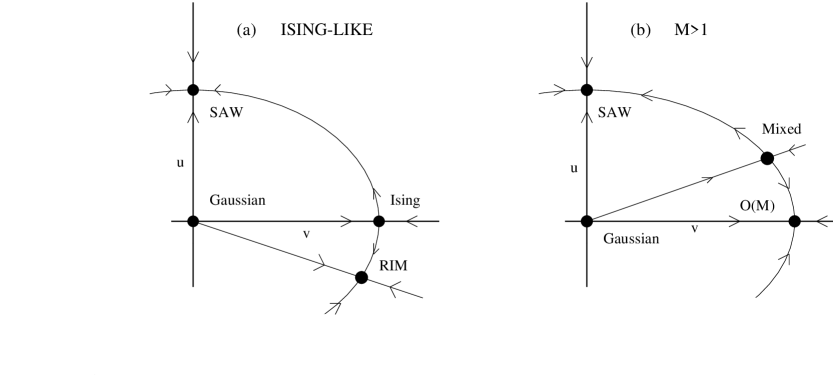
Figure 1: Scketch of the RG flow in the coupling plane $(u,v)$ for (a) Ising ($M=1$) and (b) $M$-component ($M>1$) randomly dilute systems.

The critical behavior of systems with quenched disorder is of considerable theoretical and experimental interest. A typical example is obtained by mixing a magnetic material with short-range interactions with a nonmagnetic material. These physical system can be described by the three-dimensional randomly dilute spin model

$${\cal H}_{p}=J\,\sum_{<ij>}\rho_{i}\,\rho_{j}\;s_{i}\cdot s_{j},$$ (23)

where the sum is extended over all nearest-neighbor sites, $s_{i}$ are $M$-component spin variables, and $\rho_{i}$ are uncorrelated quenched random variables, which are equal to one with probability $p$ (the spin concentration) and zero with probability $1-p$ (the impurity concentration). See, e.g., Refs. [4, 30, 2, 31] for reviews discussing these systems. For sufficiently low spin dilution $1-p$, i.e. above the percolation threshold of the spin concentration, the system described by the Hamiltonian ${\cal H}_{p}$ undergoes a second-order phase transition at $T_{c}(p)<T_{c}(p=1)$.

The critical behavior of randomly dilute spin systems is rather well established. Randomly dilute Ising systems, of which the random Ising model (RIM) (23) is an example, belong to a new universality class which is distinct from the Ising universality class describing the critical behavior of the pure system. This has been clearly observed in experiments on dilute uniaxial antiferromagnets such as Fe_xZn_1-xF₂ and Mn_xZn_1-xF₂ materials. The critical exponents turn out to be independent from the impurity concentration and definitely different from those of the pure Ising universality class, see, e.g., their estimates reported in Refs. [30, 2, 31]. In these antiferromagnetic systems the presence of a uniform magnetic field causes a crossover to a different random-field critical behavior [32]. These experimental result are confirmed by renormalization-group studies, showing that the pure Ising FP is unstable with respect to the addition of impurities and that the critical behavior is controlled by a new stable RIM FP.

Unlike Ising-like systems, multicomponent O($M$)-symmetric spin systems do not change their asymptotic critical behavior in the presence of random impurities. This is predicted by the Harris criterion [33] which states that the addition of impurities to a system which undergoes a continuous transition does not change its critical behavior if the specific-heat critical exponent $\alpha$ of the pure system is negative. For $M>1$ the specific-heat exponent $\alpha_{M}$ of the pure system is negative, for example [16, 17] $\alpha_{2}\approx-0.014$ and $\alpha_{3}\approx-0.13$, respectively for the XY and Heisenberg universality classes, and thus disorder is irrelevant. From the RG point of view, the Wilson-Fisher FP of the pure O($M$) theory is stable under the perturbation induced by the dilution. The presence of impurities affects only the approach to the critical regime, leaving the asymptotic behavior unchanged. This is confirmed by several experiments that investigated the effect of disorder on the $\lambda$-transition of ⁴He (it belongs to the XY universality class) [34, 35, 2] and on Heisenberg magnets [36, 37, 38].

The FT approach is based on an effective translation-invariant LGW Hamiltonian that is obtained by using the replica method [39, 40, 41, 42], i.e.

$${\cal H}_{MN}=\int d^{d}x\left\{\sum_{ia}{1\over 2}\left[(\partial_{\mu}\Phi_{ai})^{2}+r\Phi_{ai}^{2}\right]+\sum_{ijab}{1\over 4!}\left(u_{0}+v_{0}\delta_{ij}\right)\Phi^{2}_{ai}\Phi^{2}_{bj}\right\}\;,$$ (24)

where $a,b=1,...M$ and $i,j=1,...N$. In the limit $N\rightarrow 0$ the Hamiltonian ${\cal H}_{MN}$ with $u_{0}<0$ and $v_{0}>0$ is expected to describe the critical properties of dilute $M$-component spin systems. Thus, their critical behavior can be investigated by studying the RG flow of ${\cal H}_{MN}$ in the limit $N\rightarrow 0$. For generic values of $M$ and $N$, the Hamiltonian ${\cal H}_{MN}$ describes $M$ coupled $N$-vector models and it is usually called $MN$ model [4]. Figure 1 sketches the expected flow diagram in the quartic-coupling plane, for Ising ($M=1$) and multicomponent ($M>1$) systems in the limit $N\rightarrow 0$. There are four FP’s: the trivial Gaussian one, an O($M$)-symmetric FP, a self-avoiding walk (SAW) FP, and a mixed FP. The SAW FP is stable and corresponds to the $(M\times N)$-vector theory for $N\rightarrow 0$; but it is not of interest for the critical behavior of randomly dilute spin models, since it is located in the region $u>0$, while the region relevant for quenched disordered systems corresponds to negative values of the coupling $u$. The stability of the other FP’s depends on the value of $M$. Nonperturbative arguments [43, 4] show that the stability of the O($M$) FP is related to the specific-heat critical exponent of the O($M$)-symmetric theory. Indeed, ${\cal H}_{MN}$ at the O($M$)-symmetric FP can be interpreted as the Hamiltonian of $N$ $M$-vector systems coupled by the O($MN$)-symmetric term. Since this interaction is the sum of the products of the energy operators of the different $M$-vector models, the crossover exponent associated with the O($MN$)-symmetric quartic interaction is given by the specific-heat critical exponent $\alpha_{M}$ of the $M$-vector model, independently of $N$. This implies that for $M=1$ (Ising-like systems) the pure Ising FP is unstable since $\phi=\alpha_{1}>0$, while for $M>1$ the O($M$) FP is stable given that $\alpha_{M}<0$, in agreement with the Harris criterion. For $M>1$ the mixed FP is in the region of positive $u$ and is unstable [4]. Therefore, the RG flow of the $M$-component model with $M>1$ is driven towards the pure O($M$) FP. Thus, the asymptotic behavior remains unchanged when impurities are added. But their effect is not totally negligible because they give rise to slowly-decaying scaling corrections proportional to $t^{\Delta}_{r}$ with $\Delta_{r}=-\alpha_{M}$, where $\alpha_{M}$ is the specific-heat exponent of the pure O($M$)-symmetric theory. For Ising-like systems, the pure Ising FP is instead unstable, and the flow for negative values of the quartic coupling $u$ leads to the stable mixed or random (RIM) FP which is located in the region of negative values of $u$. The above picture emerges clearly in the framework of the $\epsilon$ expansion, although the RIM FP is of order $\sqrt{\epsilon}$ [44] rather than $\epsilon$.

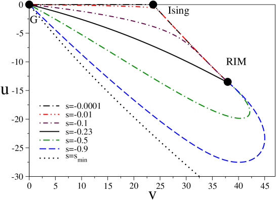
Figure 2: RG trajectories in the $u,v$ plane for various values of $s\equiv u_{0}/v_{0}<0$. From Ref. [45].

The most precise FT results have been obtained in the framework of the FD expansion in powers of the zero-momentum quartic couplings related to $u_{0}$ and $v_{0}$. In this scheme the theory is renormalized by introducing a set of zero-momentum conditions for the one-particle irreducible two-point and four-point correlation functions, which relate the zero-momentum mass scale $m$ and the quartic couplings $u$ and $v$ to the corresponding Hamiltonian parameters $r$, $u_{0}$, and $v_{0}$. This is just a straightforward extension of the method outlined in Sec. 2.1 to a theory with two quartic parameters. The critical behavior of dilute spin systems is determined by the stable FP of the theory, that is given by the common zero $u^{*},v^{*}$ of the $\beta$-functions in the limit $N\rightarrow 0$

$$\beta_{u}(u,v)=\left.m{\partial u\over\partial m}\right|_{u_{0},v_{0}},\qquad\beta_{v}(u,v)=\left.m{\partial v\over\partial m}\right|_{u_{0},v_{0}},$$ (25)

whose stability matrix has positive eigenvalues (actually a positive real part is sufficient). Then, the critical exponents are obtained by evaluating appropriate RG functions at $u^{*},v^{*}$. Figs. 2 and 3 show typical RG trajectories in the zero-momentum quartic plane $u$, $v$ in the relevant region corresponding to $u_{0}<0$, for the RIM and the random Heisenberg model respectively [45].

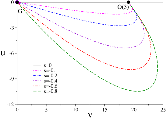
Figure 3: RG trajectories of the dilute Heisenberg model for various values of $s\equiv u_{0}/v_{0}<0$. From Ref. [45].

The FD expansions of the $\beta$ functions and of the critical exponents have been computed to six loops [46, 24, 47]. The results of the six-loop analyses are reported in Table 3, where they are compared with estimates obtained in Monte Carlo simulations of the RIM, see, e.g., Refs. [48, 49], and in experiments on uniaxial antiferromagnets, such as Fe_xZn_1-xF₂ and Mn_xZn_1-xF₂, see, e.g., Refs. [30, 31]. The agreement is satisfactory, although we note the slightly smaller value of the experimental estimate of $\alpha$. We mention that several computations have also been done in the framework of the $\epsilon$ expansion. The $\sqrt{\epsilon}$ expansion [44] turns out not to be effective for a quantitative study of the RIM (see, e.g., the analysis of the five-loop series done in Ref. [50]). The related minimal-subtraction renormalization scheme without $\epsilon$ expansion [8] have been also considered. The three- and four-loop results turn out to be in reasonable agreement with the estimates obtained by other methods, but at five loops no random FP is found [51]. Nonperturbative approaches based on scaling-field expansions and on continuous RG equations have also been exploited [52, 53], providing substantially consistent results. A more complete list of theoretical and experimental results can be found in Refs. [2, 30, 31].

Table 3: Critical exponents for the RIM universality class.

		$\gamma$	$\nu$	$\alpha$	$\beta$
six-loop FD	[46]	1.330(17)	0.678(10)	$-$0.034(30)	0.349(5)
Monte Carlo	[48]	1.342(6)	0.683(3)	$-$0.049(9)	0.3534(15)
FexZn1-xF2	[30]	1.31(3)	0.69(1)	$-$0.10(2)	0.359(9)

Using the FT approach, one can also compute the critical exponent $\phi$ describing the crossover from random-dilution to random-field critical behavior in Ising systems, and in particular the crossover observed in dilute anisotropic antiferromagnets when an external magnetic field is applied [30]. The crossover exponent $\phi$ is related to the RG dimensions of the quadratic operator $\Phi_{i}\Phi_{j}$ ($i\neq j$) in the limit $N\rightarrow 0$ [54]. Six-loop computations [55] provide the estimate $\phi=1.42(2)$, which is in good agreement with the available experimental estimates, for example $\phi=1.42(3)$ for Fe_xZn_1-xF₂ [30].

Finally, we mention that a perturbative six-loop analysis of the combined effect of impurities and magnetic anisotropy has been reported in Ref. [29].

5 Frustrated spin models with noncollinear order

In physical magnets noncollinear order is due to frustration that may arise either because of the special geometry of the lattice, or from the competition of different kinds of interactions [56]. Typical examples of systems of the first type are stacked triangular antiferromagnets (STA’s), where magnetic ions are located at each site of a three-dimensional stacked triangular lattice. On the basis of the structure of the ground state, in an $N$-component STA one expects a transition associated with the breakdown of the symmetry from O($N$) in the HT phase to O($N-2$) in the LT phase. The nature of the transition, and in particular the existence of a new chiral universality class [57], is still controversial. On this issue, there is still much debate, FT methods, Monte Carlo simulations, and experiments providing contradictory results in many cases (see, e.g., Ref.[2] for a recent review of results). Overall, experiments on STA’s favor a continuous transition belonging to a new chiral universality class.

The determination of an effective LGW Hamiltonian describing the critical behavior leads to the O($M$)$\otimes$O($N$)-symmetric theory [57]

$${\cal H}_{ch}=\int d^{d}x\Bigl{\{}{1\over 2}\sum_{a}\Bigl{[}(\partial_{\mu}\phi_{a})^{2}+r\phi_{a}^{2}\Bigr{]}+{1\over 4!}u\Bigl{(}\sum_{a}\phi_{a}^{2}\Bigr{)}^{2}+{1\over 4!}v\sum_{a,b}\Bigl{[}(\phi_{a}\cdot\phi_{b})^{2}-\phi_{a}^{2}\phi_{b}^{2}\Bigr{]}\Bigr{\}},$$ (26)

where $\phi_{a}$, $a=1,\ldots,M$, are $N$-component vectors. The case $M=2$ with $v>0$ describes frustrated spin models with noncollinear order. Negative values of $v$ correspond to magnets with sinusoidal spin structures. XY and Heisenberg systems correspond to $N=2$ and $N=3$ respectively. Recently the Hamiltonian (26) has also been considered to discuss the phase diagram of Mott insulators [58]. See Refs. [56, 2] for other applications.

Six-loop calculations [59] in the framework of the $d=3$ FD expansion provide a rather robust evidence for the existence of a new stable FP in the XY and Heisenberg cases corresponding to the conjectured chiral universality class, contradicting earlier studies based on much shorter (three-loop) series [60]. It has also been argued [61] that the stable chiral FP is actually a focus, due to the fact that the eigenvalues of its stability matrix turn out to have a nonzero imaginary part. The new chiral FP’s found for $N=2,3$ should describe the apparently continuous transitions observed in STA’s. The FT estimates of the critical exponents are in satisfactory agreement with the experimental results, including the chiral crossover exponent related to the chiral degrees of freedom [62].

On the other hand, other FT studies, see, e.g., Refs. [63, 64], based on approximate solutions of continuous RG equations, do not find a stable FP, thus favoring a weak first-order transition. Monte Carlo simulations have not been conclusive in setting the question, see, e.g., Refs. [65, 66, 67]. Since all the above approaches rely on different approximations and assumptions, their comparison and consistency is essential before considering the issue substantially understood.

Finally, we mention that the six-loop FT analysis of the critical behavior of systems with nonplanar ordering, i.e. with $M\geq 3$, has not find any evidence of the presence of a stable FP [68], suggesting a first-order transition. A high-order FT study of two-dimensional systems have been reported in Ref. [69].

6 Competition of two distinct order parameters

The competition of distinct types of ordering gives rise to multicritical behavior. More specifically, a multicritical point (MCP) is observed at the intersection of two critical lines characterized by different order parameters. MCP’s arise in several physical contexts. The phase diagram of anisotropic antiferromagnets in a uniform magnetic field $H_{\parallel}$ parallel to the anisotropy axis presents two critical lines in the temperature-$H_{\parallel}$ plane, belonging to the XY and Ising universality classes, that meet at a MCP [70, 5]. MCP’s are also expected in the temperature-doping phase diagram of high-$T_{c}$ superconductors. Within the SO(5) theory [71, 72] of high-$T_{c}$ superconductivity, it has been speculated that the antiferromagnetic and superconducting transition lines meet at a MCP in the temperature-doping phase diagram.

Different phase diagrams have been observed close to a MCP. If the transition at the MCP is continuous, one may observe either a bicritical or a tetracritical behavior. A bicritical behavior is characterized by the presence of a first-order line that starts at the MCP and separates the two different ordered low-temperature phases, see Fig. 4. In the tetracritical case, there exists a mixed low-temperature phase in which both types of ordering coexist and which is bounded by two critical lines meeting at the MCP, see Fig. 5. It is also possible that the transition at the MCP is of first order. A possible phase diagram is sketched in Fig. 6. In this case the two first-order lines, which start at the MCP and separate the disordered phase from the ordered phases, end in tricritical points and then continue as critical lines.

6.1 Multicritical behavior in O($n_{1}$)$\oplus$O($n_{2}$) theories

The multicritical behavior arising from the competition of two types of ordering characterized by O($n$) symmetries is determined by the RG flow of the most general O($n_{1}$)$\oplus$O($n_{2}$)-symmetric LGW Hamiltonian involving two fields $\phi_{1}$ and $\phi_{2}$ with $n_{1}$ and $n_{2}$ components respectively, i.e. [5]

$${\cal H}_{mc}= \int d^{d}x\Bigl{[}{\textstyle\frac{1}{2}}(\partial_{\mu}\phi_{1})^{2}+{\textstyle\frac{1}{2}}(\partial_{\mu}\phi_{2})^{2}+{\textstyle\frac{1}{2}}r_{1}\phi_{1}^{2}+{\textstyle\frac{1}{2}}r_{2}\phi_{2}^{2}$$

$$+u_{1}(\phi_{1}^{2})^{2}+u_{2}(\phi_{2}^{2})^{2}+w\phi_{1}^{2}\phi_{2}^{2}\Bigr{]}.$$

The critical behavior at the MCP is determined by the stable FP when both $r_{1}$ and $r_{2}$ are tuned to their critical value. An interesting possibility is that the stable FP has O($N$) symmetry, $N\equiv n_{1}+n_{2}$, so that the symmetry gets effectively enlarged approaching the MCP. As we shall see, this is realized only in the case $N=2$, i.e. when two Ising lines meet.

The phase diagram of the model with Hamiltonian (6.1) has been investigated within the mean-field approximation in Ref. [73]. If the transition at the MCP is continuous, one may observe either a bicritical or a tetracritical behavior. But it is also possible that the transition at the MCP is of first order. A low-order calculation in the framework of the $\epsilon$ expansion [5] shows that the isotropic O($N$)-symmetric FP ($N\equiv n_{1}+n_{2}$) is stable for $N<N_{c}=4-2\epsilon+O(\epsilon^{2})$. With increasing $N$, a new FP named biconal FP (BFP), which has only O($n_{1}$)$\oplus$O($n_{2}$) symmetry, becomes stable. Finally, for large $N$, the decoupled FP (DFP) is the stable FP. In this case, the two order parameters are effectively uncoupled at the MCP. The extension of these $O(\epsilon)$ results to three dimensions suggests that for $n_{1}=1$ and $n_{2}=2$, the case relevant for anisotropic antiferromagnets, the MCP belongs to the O(3) universality class, while for $n_{1}=2$ and $n_{2}=3$, of relevance for the SO(5) theory of high-$T_{c}$ superconductivity, the stable FP is the BFP.

Figure 4: Phase diagram in the plane $T$-$g$ presenting a bicritical point. Here, $T$ is the temperature and $g$ a second relevant parameter. The thick line (“flop line”) represents a first-order transition.

Figure 5: Phase diagram with a tetracritical point.

Figure 6: Phase diagram with a first-order MCP. The thick lines represent first-order transitions.

The $O(\epsilon)$ computations provide useful indications on the RG flow in three dimensions, but a controlled extrapolation to $\epsilon=1$ requires much longer series and an accurate resummation exploiting their Borel summability. This has been recently achieved, extending the $\epsilon$ expansion to $O(\epsilon^{5})$ [23]. A robust picture of the RG flow predicted by the O($n_{1}$)$\oplus$O($n_{2}$)-symmetric LGW theory has been achieved by supplementing the analysis of the $\epsilon$ series with the results for the stability of the O($N$) FP (cf. Sec. 3), which were also obtained by analyzing six-loop FD series, and with nonperturbative arguments allowing to establish the stability of the DFP [74, 75].

In order to establish the stability properties of the O($N$) symmetric FP, we first note that the Hamiltonian (6.1) contains combinations of spin-2 and spin-4 polynomial operators that are invariant under the symmetry O($n_{1}$)$\oplus$O($n_{2}$). Explicitly, they are given by

$${\cal P}_{2,0}=\Phi^{2},\qquad\qquad{\cal P}_{2,2}=\sum_{a=1}^{n_{1}}P_{2,2}^{aa}=\phi_{1}^{2}-{n_{1}\over N}\Phi^{2},$$ (28)

$${\cal P}_{4,0}=(\Phi^{2})^{2},\qquad\qquad{\cal P}_{4,2}=\Phi^{2}{\cal P}_{2,2},$$

$${\cal P}_{4,4}=\sum_{a=1}^{n_{1}}\sum_{b=n_{1}+1}^{n_{2}}P_{4,4}^{aabb}=\phi_{1}^{2}\phi_{2}^{2}-{\Phi^{2}(n_{1}\phi_{2}^{2}+n_{2}\phi_{1}^{2})\over N+4}+{n_{1}n_{2}(\Phi^{2})^{2}\over(N+2)(N+4)},$$

where $\Phi$ is the $N$-component field $(\phi_{1},\phi_{2})$. The RG dimension $y_{2,2}$ of ${\cal P}_{2,2}$, and therefore of the operator $P_{2,2}^{ab}$ (see Table 2), provides the crossover exponent $\phi=y_{2,2}\nu$ at the MCP. Concerning the fourth-order terms, the results for the spin-4 RG dimension $y_{4,4}$ at the O($N$) FP (see again Table 2) imply that the O($N$) FP is stable only for $N=2$, i.e. when two Ising-like critical lines meet. It is unstable in all cases with $N\geq 3$. This implies that for $N\geq 3$ the enlargement of the symmetry O($n_{1}$)$\oplus$O($n_{2}$) to O($N$) does not occur, unless an additional parameter is tuned beside those associated with the quadratic perturbations.

The analysis of the five-loop $\epsilon$ series shows that for $N=3$, i.e. for $n_{1}=1$ and $n_{2}=2$, the critical behavior at the MCP is described by the BFP, whose critical exponents turn out to be very close to those of the Heisenberg universality class. For $N\geq 4$ and for any $n_{1},n_{2}$ the DFP is stable, implying a tetracritical behavior. This can also be inferred by using nonperturbative arguments [74, 75] that allow to determine the relevant stability eigenvalue from the critical exponents of the O($n_{i}$) universality classes. At the DFP, the dominant perturbation is the quartic coupling term $w\phi_{1}^{2}\phi_{2}^{2}$ that scales as the product of two energy-like operators, which have RG dimensions $(1-\alpha_{i})/\nu_{i}$ where $\alpha_{i}$ and $\nu_{i}$ are the critical exponents of the O($n_{i}$) universality classes. Therefore, the RG dimension related to the $w$-perturbation is given by

$$y_{w}={\alpha_{1}\over 2\nu_{1}}+{\alpha_{2}\over 2\nu_{2}}={1\over\nu_{1}}+{1\over\nu_{2}}-d.$$ (29)

The stability properties of the DFP can be established by determining the sign of $y_{w}$. Using the estimates of the critical exponents of the three-dimensional O($n_{i}$) universality classes, see Sec. 2, $y_{w}$ turns out to be negative for $N\equiv n_{1}+n_{2}\geq 4$, and positive for $N=2,3$. Therefore, the DFP turns out to be stable for $N\geq 4$. Finally, when the initial parameters of the Hamiltonian are not in the attraction domain of the stable FP, the transition between the disordered and ordered phases should be of first order in the neighborhood of the MCP. In this case, a possible phase diagram is given in Fig. 6, where all transition lines are first-order close to the MCP.

6.2 Anisotropic antiferromagnets in a uniform magnetic field

Anisotropic antiferromagnets in a uniform magnetic field $H_{\parallel}$ parallel to the anisotropy axis present a MCP in the $T-H_{\parallel}$ phase diagram, where two critical lines belonging to the XY and Ising universality classes meet [5]. In this case the high-order FT analyses predict a multicritical behavior described by the BFP, in contrast with earlier low-order $\epsilon$-expansion calculations [5] that predicted the enlargement of the symmetry to O(3). The mean-field approximation assigns a tetracritical behavior to the MCP [5], but a more rigorous characterization, that requires the computation of the corresponding scaling free energy, is needed to draw a definite conclusion. Experimentally, the MCP appears to be bicritical, see, e.g., Refs. [76, 77]. A quantitative analysis of the biconal FP shows that its critical exponents are very close to the Heisenberg ones. For instance, the correlation-length exponent $\nu$ differs by less than 0.001 in the two cases. Thus, it should be very hard to distinguish the biconal from the O(3) critical behavior in experiments or numerical works based on Monte Carlo simulations. The crossover exponent describing the crossover from the O(3) critical behavior is very small, i.e., $\phi_{4,4}=y_{4,4}\nu\approx 0.01$, see Table 2, so that systems with a small effective breaking of the O(3) symmetry show a very slow crossover towards the biconal critical behavior or, if the system is outside the attraction domain of the BFP, towards a first-order transition; thus, they may show the eventual asymptotic behavior only for very small values of the reduced temperature.

6.3 Nature of the multicritical point within the SO(5) theory of high-$T_{c}$ superconductors.

High-$T_{c}$ superconductors are other interesting physical systems in which MCP’s may arise from the competition of different order parameters. At low temperatures these materials exhibit superconductivity and antiferromagnetism depending on doping. The SO(5) theory [71, 72] attempts to provide a unified description of these two phenomena, by introducing a three-component antiferromagnetic order parameter and a $d$-wave superconducting order parameter with U(1) symmetry, with an approximate O(5) symmetry. This theory predicts a MCP arising from the competition of these two order parameters when the corresponding critical lines meet in the temperature-doping phase diagram. Neglecting the fluctuations of the magnetic field and the quenched randomness introduced by doping, see, e.g., Ref. [75] for a critical discussion of this point, one may consider the O(3)$\oplus$O(2)-symmetric LGW Hamiltonian to infer the critical behavior at the MCP, see, e.g., Refs. [78, 79, 80, 81, 82, 83]. In particular, the analysis of Ref. [81], which uses the projected SO(5) model as a starting point, shows that one can use Eq. (6.1) as an effective Hamiltonian.

Different scenarios have been proposed for the critical behavior at the MCP. In Refs. [71, 78, 79], it was speculated that the MCP is a bicritical point where the O(5) symmetry is asymptotically realized. This picture has been apparently supported by Monte simulations for a five-component O(3)$\oplus$O(2)-symmetric spin model [79], and by a quantum Monte Carlo study of the quantum projected SO(5) model in three dimensions [84]. These numerical studies show that, within the parameter ranges considered, the scaling behavior at the MCP is consistent with an O(5)-symmetric critical behavior. On the basis of the $O(\epsilon)$ results of Refs. [5], Refs. [80, 82] predicted a tetracritical behavior governed by the BFP. However, since the BFP was expected to be close to the O(5) FP, it was suggested that at the MCP the critical exponents were in any case close to the O(5) ones. These hypotheses are contradicted by the high-order FT results that we have discussed in Sec. 6.1. They indeed show that the DFP is the only stable FP. This implies that the asymptotic approach to the MCP is characterized by a decoupled tetracritical behavior or by a first-order transition for systems that are outside the attraction domain of the DFP. The O(5) symmetry can be asymptotically realized only by tuning a further relevant parameter, beside the double tuning required to approach the MCP. The O(5) FP is unstable with a crossover exponent $\phi_{4,4}=y_{4,4}\nu\approx 0.15$, see Table 2, which, although rather small, is nonetheless sufficiently large not to exclude the possibility of observing the RG flow towards the eventual asymptotic behavior for reasonable values of the reduced temperature. Evidence in favor of a tetracritical behavior has been recently provided by a number of experiments, see, e.g., Refs. [85, 86, 87, 88, 89, 90], which seem to show the existence of a coexistence region of the antiferromagnetic and superconductivity phases. The possible coexistence of the two phases has been discussed in Refs. [83, 91, 92].

References

- [1] J. Zinn-Justin, Quantum Field Theory and Critical Phenomena, fourth edition (Clarendon Press, Oxford, 2002).
- [2] A. Pelissetto, E. Vicari, Phys. Rep. 368 (2002) 549.
- [3] E. Brézin, J.C. Le Guillou, J. Zinn-Justin, in Phase Transitions and Critical Phenomena, edited by C. Domb and M.S. Green (Academic Press, New York, 1976), Vol. 6, p. 125.
- [4] A. Aharony, in Phase Transitions and Critical Phenomena, edited by C. Domb and M.S. Green (Academic Press, New York, 1976), Vol. 6, p. 357.
- [5] D.R. Nelson, J.M. Kosterlitz, M.E. Fisher, Phys. Rev. Lett. 33 (1974) 813. J.M. Kosterlitz, D.R. Nelson, M.E. Fisher, Phys. Rev. B 13 (1976) 412.
- [6] K.G. Wilson, M.E. Fisher, Phys. Rev. Lett. 28 (1972) 240.
- [7] G. Parisi, Cargèse Lectures (1973), J. Stat. Phys. 23 (1980) 49.
- [8] V. Dohm, Z. Phys. B 60 (1985) 61; B 61 (1985) 193. R. Schloms, V. Dohm, Nucl. Phys. B 328 (1989) 639.
- [9] C. Bagnuls, C. Bervillier, Phys. Rev. B 32 (1985) 7209.
- [10] G.A. Baker, Jr., B.G. Nickel, M.S. Green, D.I. Meiron, Phys. Rev. Lett. 36 (1977) 1351; G.A. Baker, Jr., B.G. Nickel, D.I. Meiron, Phys. Rev. B 17 (1978) 1365.
- [11] D.B. Murray, B.G. Nickel, “Revised estimates for critical exponents for the continuum -vector model in 3 dimensions,” unpublished Guelph University report (1991).
- [12] J.C. Le Guillou, J. Zinn-Justin, Phys. Rev. Lett. 39 (1977) 95; Phys. Rev. B 21 (1980) 3976.
- [13] R. Guida, J. Zinn-Justin, J. Phys. A 31 (1998) 8103.
- [14] M. Campostrini, A. Pelissetto, P. Rossi, E. Vicari, Phys. Rev. E 65 (2002) 066127; E 60 (1999) 3526.
- [15] M. Hasenbusch, Int. J. Mod. Phys. C 12 (2001) 911.
- [16] M. Campostrini, M. Hasenbusch, A. Pelissetto, P. Rossi, E. Vicari, Phys. Rev. B 63 (2001) 214503.
- [17] M. Campostrini, M. Hasenbusch, A. Pelissetto, P. Rossi, E. Vicari, Phys. Rev. B 65 (2002) 144520.
- [18] G. ’t Hooft, M.J.G. Veltman, Nucl. Phys. B 44 (1972) 189.
- [19] K.G. Chetyrkin, S.G. Gorishny, S.A. Larin, F.V. Tkachov, Phys. Lett. B 132 (1983) 351.
- [20] H. Kleinert, J. Neu, V. Schulte-Frohlinde, K.G. Chetyrkin, S.A. Larin, Phys. Lett. B 272 (1991) 39; (E) B 319 (1993) 545.
- [21] F. J. Wegner, Phys. Rev. B 6 (1972) 1981.
- [22] P. Calabrese, A. Pelissetto, E. Vicari, Phys. Rev. E 65 (2002) 046115.
- [23] P. Calabrese, A. Pelissetto, E. Vicari, Phys. Rev. B 67 (2003) 054505; cond-mat/0203533.
- [24] J.M. Carmona, A. Pelissetto, E. Vicari, Phys. Rev. B 61 (2000) 15136.
- [25] M. De Prato, A. Pelissetto, E. Vicari, cond-mat/0302145.
- [26] S. Chikazumi, Physics of Ferromagnetism (Clarendon, Oxford, 1997) Chapt. 12.
- [27] R. Folk, Yu. Holovatch, T. Yavors’kii, Phys. Rev. B 62 (2000) 12195; (E) B 63 (2001) 189901.
- [28] H. Kleinert, V. Schulte-Frohlinde, Phys. Lett. B 342 (1995) 284.
- [29] P. Calabrese, A. Pelissetto, E. Vicari, Phys. Rev. B 67 (2003) 024418.
- [30] D.P. Belanger, Brazilian J. Phys. 30 (2000) 682 [cond-mat/0009029]; in Spin Glasses and Random Fields, edited by A.P. Young (World Scientific, Singapore, 1998), p. 251 [cond-mat/9706042].
- [31] R. Folk, Yu. Holovatch, T. Yavors’kii, Uspekhi Fiz. Nauk 173 (2003) 175 [Physics Uspekhi 46 (2003) 175 [cond-mat/0106468].
- [32] S. Fishman, A. Aharony, J. Phys. C 12, L729 (1979). D.P. Belanger, in Spin Glasses and Random Fields, edited by A. P. Young (World Scientific, Singapore, 1998), p. 251 [cond-mat/9706042].
- [33] A.B. Harris, J. Phys. C 7 (1974) 1671.
- [34] J. Yoon, M.H.W. Chan, Phys. Rev. Lett. 78 (1997) 4801.
- [35] G.M. Zassenhaus, J.D. Reppy, Phys. Rev. Lett. 83 (1999) 4800.
- [36] S. N. Kaul, J. Magn. Magn. Mater. 53 (1985) 5.
- [37] S. N. Kaul, M. Sambasiva Rao, J. Phys.: Condens. Matter 6 (1994) 7403.
- [38] P.D. Babu, S.N. Kaul, J. Phys.: Condens. Matter 9 (1997) 7189.
- [39] V.J. Emery, Phys. Rev. B 11 (1975) 239.
- [40] S.W. Edwards, P.W. Anderson, J. Phys. F 5 (1975) 965.
- [41] G. Grinstein, A. Luther, Phys. Rev. B 13 (1976) 1329.
- [42] A. Aharony, Y. Imry, S.K. Ma, Phys. Rev. B 13 (1976) 466.
- [43] J. Sak, Phys. Rev. B 10 (1974) 3957.
- [44] D. E. Khmelnitskii, Zh. Eksp. Teor. Fiz. 68 (1975) 1960 [Sov. Phys. JETP 41 (1976) 981].
- [45] P. Calabrese, P. Parruccini, A. Pelissetto, E. Vicari, in preparation.
- [46] A. Pelissetto, E. Vicari, Phys. Rev. B 62 (2000) 6393.
- [47] D.V. Pakhnin, A.I. Sokolov, Phys. Rev. B 61 (2000) 15130.
- [48] P. Calabrese, V. Martín-Mayor, A. Pelissetto, E. Vicari, cond-mat/0306272.
- [49] H.G. Ballesteros, L.A. Fernández, V. Martín-Mayor, A. Muñoz Sudupe, G. Parisi, J.J. Ruiz-Lorenzo, Phys. Rev. B 58 (1998) 2740.
- [50] B. N. Shalaev, S. A. Antonenko, A. I. Sokolov, Phys. Lett. A 230 (1997) 105.
- [51] R. Folk, Yu. Holovatch, T. Yavors’kii, Phys. Rev. B 61 (2000) 15114.
- [52] K. E. Newman, E. K. Riedel, Phys. Rev. B 25 (1982) 264.
- [53] M. Tissier, D. Mouhanna, J. Vidal, B. Delamotte, Phys. Rev. B 65 (2002) 140402.
- [54] A. Aharony, Europhys. Lett. 1 (1986) 617.
- [55] P. Calabrese, A. Pelissetto, E. Vicari, cond-mat/0305041.
- [56] H. Kawamura, J. Phys.: Condens. Matter 10 (1998) 4707.
- [57] H. Kawamura, Phys. Rev. B 38 (1988) 4916; (E) B 42 (1990) 2610.
- [58] S. Sachdev, Ann. of Phys. (San Diego) 303 (2003) 226; cond-mat/0211005.
- [59] A. Pelissetto, P. Rossi, E. Vicari, Phys. Rev. B 63 (2001) 140414(R); Nucl. Phys. B 607 (2001) 605.
- [60] S.A. Antonenko, A.I. Sokolov, Phys. Rev. B 49 (1994) 15901.
- [61] P. Calabrese, P. Parruccini, A.I. Sokolov, Phys. Rev. B 66 (2002) 180403(R); cond-mat/0304154.
- [62] A. Pelissetto, P. Rossi, E. Vicari, Phys. Rev. B 65 (2002) 020403(R).
- [63] G. Zumbach, Phys. Rev. Lett. 71 (1993) 2421; Nucl. Phys. B 413 (1994) 771.
- [64] M. Tissier, B. Delamotte, D. Mouhanna, Phys. Rev. Lett. 84 (2000) 5208; Phys. Rev. B 67 (2003) 134422.
- [65] D. Loison, K.D. Schotte, Eur. Phys. J. B 5 (1998) 735; B 14 (2000) 125.
- [66] M. Itakura, J. Phys. Soc. Jpn. 72 (2003) 74.
- [67] A. Peles, B.W. Southern, Phys. Rev. B 67 (2003) 184407.
- [68] P. Parruccini, cond-mat/0305287.
- [69] P. Calabrese, P. Parruccini, Phys. Rev. B 64 (2001) 184408. P. Calabrese, E.V. Orlov, P. Parruccini, A.I. Sokolov, Phys. Rev. B 67 (2003) 024413.
- [70] M.E. Fisher, D.R. Nelson, Phys. Rev. Lett. 32 (1974) 1350.
- [71] S.-C. Zhang, Science 275 (1997) 1089.
- [72] S.-C. Zhang, J.-P. Hu, E. Arrigoni, W. Hanke, A. Auerbach, Phys. Rev. B 60 (1999) 13070.
- [73] K.-S. Liu, M.E. Fisher, J. Low Temp. Phys. 10 (1972) 655.
- [74] A. Aharony, Phys. Rev. Lett. 88 (2002) 059703.
- [75] A. Aharony, J. Stat. Phys. 110 (2003) 659.
- [76] H. Rohrer, Ch. Gerber, Phys. Rev. Lett. 38 (1977) 909.
- [77] A.R. King, H. Rohrer, Phys. Rev. B 19 (1979) 5864.
- [78] J.-P. Hu, S.-C. Zhang, Physica C 341 (2000) 93.
- [79] X. Hu, Phys. Rev. Lett. 87 (2001) 057004; 88 (2002) 059704.
- [80] C.P. Burgess, C.A. Lütken, Phys. Rev. B 57 (1998) 8642.
- [81] E. Arrigoni, W. Hanke, Phys. Rev. Lett. 82 (1999) 2115; Phys. Rev. B 62 (2000) 11770.
- [82] S. Murakami, N. Nagaosa, J. Phys. Soc. Jpn. 69 (2000) 2395.
- [83] S.A. Kivelson, G. Aeppli, V.J. Emery, Proc. Natl. Acad. Sci. USA 98 (2001) 11903.
- [84] A. Dorneich, E. Arrigoni, M. Jöstingmeier, W. Hanke, S.-C. Zhang, cond-mat/0207528.
- [85] B. Khaykovich, Y. S. Lee, R.W. Erwin, S.-H. Lee, S. Wakamoto, K. J. Thomas, M. A. Kastner, R.J. Birgeneau, Phys. Rev. B 66 (2002) 014528.
- [86] Y. S. Lee, R.J. Birgeneau, M.A. Kastner, Y. Endoh, S. Wakimoto, K. Yamada, R.W. Erwin, S.-H. Lee, G. Shirane, Phys. Rev. B 60 (1999) 3643.
- [87] S. Katano, M. Sato, K. Yamada, T. Suzuki, T. Fukase, Phys. Rev. B 62 (2000) R14677.
- [88] R.I. Miller, R.F. Kiefl, J.H. Brewer, J. E. Sonier, J. Chakhalian, S. Dunsiger, G.D. Morris, A.N. Price, D.A. Bonn, W.H. Hardy, R. Liang, Phys. Rev. Lett. 88 (2002) 137002.
- [89] B. Lake, G. Aeppli, K.N. Clausen, D.F. McMorrow, K. Lefmann, N.E. Hussey,, N. Mangkorntong, M. Nohara, H. Takagi, T.E. Mason, A. Schröder, Science 291 (2001) 1759.
- [90] G. Aeppli, T.E. Mason, S.M. Hayden, H.A. Mook, J. Kulda, Science 288 (2000) 475.
- [91] Y. Zhang, E. Demler, S. Sachdev, Phys. Rev. B 66 (2002) 094501.
- [92] I. Martin, G. Ortiz, A.V. Balatsky, A.R. Bishop, Int. J. Mod. Phys. B 14 (2000) 3567.