Spatial Coherence Resonance near Pattern-Forming Instabilities

Abstract

The analogue of temporal coherence resonance for spatial degrees of freedom is reported. Specifically, we show that spatiotemporal noise is able to optimally extract an intrinsic spatial scale in nonlinear media close to (but before) a pattern-forming instability. This effect is observed in a model of pattern-forming chemical reaction and in the Swift-Hohenberg model of fluid convection. In the latter case, the phenomenon is described analytically via an approximate approach.

The ability of noise to induce temporal coherence in nonlinear systems is a well documented fact. In stochastic resonance (SR), for instance, random fluctuations enhance the response to weak periodic driving, as observed in many different physical, chemical and biological scenarios wiesenfeld . From a more intriguing perspective, even systems showing no explicit time scale exhibit an enhancement of temporal coherence due to noise gang ; rappel . This autonomous stochastic resonance, where noise extracts a hidden, intrinsic time scale of the system’s dynamics, has been termed coherence resonance (CR) pikovsky , and has been predicted theoretically in a wide variety of models (see revexc for a review) and observed experimentally in fields as diverse as plasma physics i , laser dynamics jorge , electronics postnov , atom trapping wilkowski and neuroscience gu .

Parallel to the advances in the fields of stochastic and coherence resonance, recent years have witnessed an increasing interest in the dynamics of systems with spatial degrees of freedom. Much work has been devoted to analyze the enhancement of spatiotemporal order by noise nises ; alonso , and the phenomena of standard temporal SR and CR have been studied in detail in arrays of dynamical elements sr-ext ; cr-ext , where it has been shown that coupling enhances the noise-induced temporal coherence. But so far, up to our knowledge, no analogues of CR (or SR, for that matter) for spatial degrees of freedom exist. Namely, we ask ourselves if noise is able to extract and optimize an intrinsic spatial scale from a deterministically homogeneous extended medium. In this Letter we show that such spatial coherence resonance (SCR) exists close to pattern-forming instabilities, mimicking one of the mechanisms of standard (temporal) CR.

There are different mechanisms giving rise to temporal CR. In the most extended situation, CR arises as the result of a matching between the time scale associated to noise-induced escape from a stable steady state and the characteristic time scale of the phase-space trajectories outside from the immediate vicinity of the fixed point (such as what happens in excitable media pikovsky ; benji or close to a saddle-node bifurcation in phase models rappel ). A second, less studied mechanism takes place near the onset of dynamical instabilities giving rise to periodic behavior, where noise excites precursors of the bifurcation in the form of stochastic limit cycles with a well-defined peak in the power spectrum, even before the bifurcation really happens kurt85 ; omberg . Such noisy precursors exhibit an optimal coherence at an intermediate noise strength, in a way typical of coherence resonance shura . This effect has been confirmed experimentally kiss .

Analogously to the temporal case, noisy precursors of pattern-forming bifurcations have been observed, in the form of noise-induced spatial structures, in electroconvection rehberg , Rayleigh-Bénard convection wu and optics miguel , for instance. In this case, the spatial power spectrum (now structure function) of the system exhibits a well defined peak due to noise, even below the bifurcation point. In what follows, we show that noise controls the shape of this spectral peak in a manner characteristic of coherence resonance, but with the role of temporal frequency being played by spatial wave number. This allows us to define a pure spatial analogue of temporal coherence resonance. The generality of the phenomenon is illustrated through its occurrence in two different pattern-forming systems, namely an activator-inhibitor model of chemical pattern formation and the Swift-Hohenberg model of fluid convection. In the latter case the effect is interpreted analytically.

We first illustrate the phenomenon of SCR in chemical pattern formation, in particular in the case of the chlorine dioxide-iodine-malonic acid (CDIMA) reaction, which is well known to exhibit both temporal and spatial dynamics Eps98 . Experimental and theoretical studies of this reaction have concluded that the malonic acid serves only as a source of iodide, and thus the system can be described by just two variables, in the way of an activator-inhibitor model: Eps98 ; ancherlengues

$$\dot{u} = {\bf\nabla}^{2}u\,+a\,-\,c\,u\,-4\,\frac{u\,v}{(1\,+\,u^{2})}\,-\,\phi$$

$$\dot{v} = b\,\left\{{\bf\nabla}^{2}v\,+\,c\,u\,-\frac{u\,v}{(1\,+\,u^{2})}\,+\,\phi\right\}\,,$$ (1)

where $u$ and $v$ play the role of activator and inhibitor fields, corresponding to the concentrations of iodine and chlorine dioxide ions, respectively (all variables and parameters are in dimensionless units). This model describes the photosensitivity of the CDIMA reaction, with $\phi$ accounting for the illumination level, which is an externally controlled parameter. Additionally, for large differences in the diffusion coefficients of the two species this system presents a Turing instability. In particular, the model has an homogenous stable state given by $u_{h}=(a-5\phi)/(5c)$ and $v_{h}=a(1+u_{h}^{2})/(5u_{h})$, which becomes unstable versus spatial perturbations of nonzero wavenumber for $\phi<\phi_{c}$. For $a=16$, $b=301$, $c=0.6$ and $d=1.07$, the critical illumination is $\phi_{c}=2.3$ ancherlengues .

This chemical system allows for an experimental study of stochastic effects, by introducing noise in the illumination profile. In this way, for instance, it has been shown experimentally that a quenched spatial noise sustains Turing patterns in this system well beyond the deterministic bifurcation threshold ancherlengues . We now consider a spatiotemporally stochastic illumination profile, $\phi\to\phi\,+\,\xi$, where $\xi(\vec{x},t)$ is a Gaussian noise with zero mean, white in time and with spatial autocorrelation given by

$$\langle\xi(\vec{x},t)\xi(\vec{x}^{\prime},t^{\prime})\rangle\,=\,2\,\sigma^{2}\,C(\vec{x}-\vec{x}^{\prime})\,\delta(t-t^{\prime}).$$ (2)

In order to examine the spatial response of the system in the presence of noise, we evaluate the structure function of the activator variable, defined as

$$S(\vec{k},t)\,=\,\frac{\langle\widehat{u}(\vec{k},t)\,\widehat{u}(-\vec{k},t)\rangle}{V}\,,$$ (3)

where $\widehat{u}(\vec{k},t)$ is the spatial Fourier transform of the activator field, $V$ is the d-dimensional volume of the system, and $\langle\cdots\rangle$ represents an ensemble average over noise realizations. Taking into account the spherical symmetry of this system, we compute the spherical average of the structure function as $s(k)\,=\,\int_{\Omega_{k}}d\Omega_{k}\,S(\vec{k},t)$, where $k=\left|\vec{k}\right|$ and $\Omega_{k}$ is a hyperspherical shell of radius $k$. The result is shown in Fig. 1(a) for increasing noise intensities dclevel , evaluated for a two-dimensional system and in the case of spatially white noise, i.e. $C(\vec{x}_{i}-\vec{x}_{j})\,=\,\delta_{ij}/\Delta x$. The average illumination $\phi$ to which the system is subjected is above threshold, thus for vanishing or very weak noises the system is homogeneous and the structure function does not show a well-defined peak as $k$ increases. However, increasing the noise intensity induces a peak in the structure function at $k=k_{\rm max}$, which represents a spatial noisy precursor of the pattern-forming bifurcation that occurs at $\phi=\phi_{c}$: fluctuations are capable to anticipate the instability, making the structure manifest even before the threshold has been crossed.

 

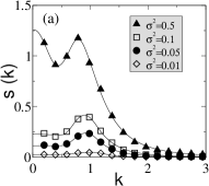
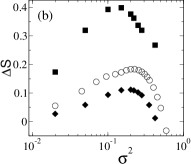
Figure 1: (a) Spherical average of the structure function for increasing noise intensities. Average illumination is $\phi=2.35$. (b) $\Delta S$ versus noise intensity for different values of the average illumination: $\phi=2.32$ (squares), $\phi=2.35$ (circles), and $\phi=2.37$ (diamonds). The simulations have been performed on a square lattice of 64$\times$64 cells with mesh size $\Delta x=0.5$.

If fluctuations become too large, disorder inevitably comes into play, and the peak in the structure function becomes less well defined [see triangles in Fig. 1(a)]. It is then clear that an optimal noise intensity exists at which the structure function peak is best resolved from the background fluctuations. In order to quantify the efficiency of the noise, an adequate measure must be used. There are different ways of quantifying such a response depending on the peculiarities of the problem under study. Here, we estimate the spatial coherence of the system through the quantity $\Delta S\equiv s(k_{\rm max})-s(0)$, taking into account that $s(0)$ measures the level of fluctuations existing in the system.

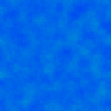
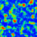
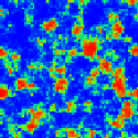
Figure 2: Spatial profiles of the activator field for increasing noise strength and $\phi=2.35$, with color mapped nonlinearly (with a $\tanh$ function) and the same contrast in all figures for comparison. From left to right, $\sigma^{2}=0.001,0.2,0.6$. The lattice parameters are those of Fig. 1.

Figure 1(b) shows how the SND varies with noise intensity $\sigma^{2}$ for different illumination levels. It can be seen that there is an optimal noise strength $\sigma^{2}_{\rm opt}$ for which the structure function peak is resolved best. This is the signature of a spatial coherence resonance driven by the external stochastic forcing, which extracts the intrinsic spatial distribution of the system. As shown in Fig. 1(b), the closer the system is to the bifurcation point, the more pronounced the resonance is, and the position of the maximum $\sigma^{2}_{\rm opt}$ shifts to smaller values.

Figure 2 shows several patterns produced by model (1) for different values of the noise strength at $\phi=2.35$. While the system is quasi-homogenous for small noise (left plot), it exhibits a rather self-organized configuration for $\sigma^{2}\sim\sigma^{2}_{\rm opt}$ (middle plot), and becomes gradually more disordered for large noise strengths (right plot). Although the effect may not appear very clear in the spatial profiles, the relevant fact is the appearance and enhancement of the peak in the structure function, since this is a measurable effect through, for instance, scattering experiments.

We may illustrate analytically this phenomenon in the case of a simpler pattern-forming model, namely the Swift-Hohenberg equation, which describes the onset of hydrodynamic convection in Rayleigh-Bénard cells cross :

$$\frac{\partial\phi(\vec{x},t)}{\partial t}=-r\phi-\phi^{3}-\left(\nabla^{2}+k_{0}^{2}\right)^{2}\phi+\xi(\vec{x},t)\,,$$ (4)

where the control parameter $r$ is proportional to the temperature gradient driving the fluid, and the additive noise $\xi(\vec{x},t)$ is again considered Gaussian and white in both time and space. As in the CDIMA model, in the absence of noise and for $r>0$, this system has a homogeneous steady state $\phi=0$, representing conduction, which upon decrease of $r$ becomes unstable at $r=r_{c}=0$ versus static perturbations of nonzero wavenumber $k=k_{0}$, which represents convection cross . In the presence of a small amount of noise, the structure function can be calculated by linearizing Eq. (4) around $\phi=0$, and transforming the system to Fourier space nises . The result is:

$$S_{st}(k)=\frac{\sigma^{2}}{(k^{2}-k_{0}^{2})^{2}+r}$$ (5)

Since we want to operate in regimes where, even though the system is deterministically homogeneous, noise can be large, we generalize the previous expression (5) by allowing the parameters $\sigma$ and $r$ to depend on noise; we will call them $\sigma^{\prime}(\sigma)$ and $r^{\prime}(\sigma)$ in what follows. In order to estimate how these renormalized parameters depend on the noise intensity, we rederive expression (5) without neglecting completely nonlinear terms. To do that, we estimate the cubic term in (4) by applying the Gaussian approximation langer $\phi(x,t)^{3}\sim 3\phi(x,t)\langle\phi^{2}\rangle_{st}$. This renders back the equation linear, so that the structure function obeys again expression (5) with $r$ being replaced by $r^{\prime}\equiv r+3\langle\phi^{2}\rangle_{st}$. We can now calculate the value of the average squared field $\langle\phi^{2}\rangle_{st}$ from the self-consistency relation

$$\langle\phi^{2}\rangle_{st} = \frac{1}{(2\pi)^{2}}\int^{\infty}_{0}S_{st}(k)2\pi k\,dk$$ (6)

$$= \frac{\pi\sigma^{2}}{(2\pi)^{2}\,\sqrt{r^{\prime}}}\left[\frac{\pi}{2}+tg^{-1}\left(\frac{k_{0}^{2}}{\sqrt{r^{\prime}}}\right)\right]\sim\frac{\sigma^{2}}{8\sqrt{r^{\prime}}}.$$

Since we will be operating close to threshold, $r$ will be small and $r^{\prime}\sim 3\langle\phi^{2}\rangle_{st}$, which leads from (6) to $\langle\phi^{2}\rangle_{st}\sim(\sigma^{2})^{2/3}$. Therefore, from the definition of $r^{\prime}$ above we finally obtain that this effective parameter also scales with noise intensity as $r^{\prime}\sim(\sigma^{2})^{2/3}$. In order to verify this result, we perform numerical simulations of model (4) in the homogeneous regime for different noise intensities, and fit the resulting structure functions with expression (5), with effective parameters $\sigma^{\prime}$ and $r^{\prime}$ which are allowed to depend on noise. The results of this analysis are shown in Fig. 3, and confirm that $\sigma^{\prime}$ scales linearly with noise intensity $\sigma$ (as expected, since nonlinear corrections did not affect this parameter in the analysis made above), whereas $r^{\prime}$ scales with noise intensity with an exponent fairly close to 2/3.

 

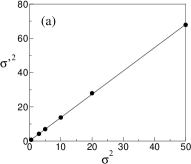
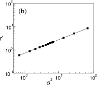
Figure 3: Effective structure-function parameters for model (4), for $r=0.05$ and $k_{0}=0.6$. In (a), the solid line corresponds to the linear relation $\sigma^{\prime 2}=1.365\sigma^{2}$, and in (b) to $r^{\prime}=0.05+a(\sigma^{2})^{\lambda}$, with $a\simeq 0.704$ and $\lambda\simeq 0.6$.

The numerical results of Fig. 4(a) have been fitted with the analytic approximation given by Eq. (5)) with renormalized parameters, leading to a quite good agreement. This is shown in Fig. 4(a) for four different noise intensities. Similarly to what occurs in the chemical model, we can see how noise excites a peak in the structure function (in this case at $k=k_{0}$) even within the homogeneous regime. This peaks increases in size as noise intensity increases, both in an absolute way and relative to the value of the structure function at $k=0$. However, for large noise intensities disorder kicks in again, and the peak becomes less pronounced.

 

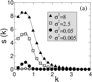
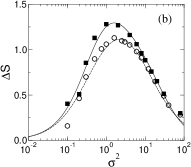
Figure 4: (a) Structure function exhibited by the Swift-Hohenberg model (4) for $r=0.005$, $k_{0}=0.6$ and four different noise intensities, listed in the legend. (b) $\Delta S$ versus noise intensity for two different values of the control parameter $r$. Squares correspond to $r=0.005$ and circles to $r=0.05$. In the two plots, lines are the fitted function (7) with the renormalized parameters given in Fig. 3. The simulations have been performed again in a square lattice of 64$\times$64 cells with spacing $\Delta x=0.5$.

This effect can be seen quantitatively, in terms of the dependence of $\Delta S$ on $\sigma^{2}$, for two different distances to threshold in Fig. 4(b), where the numerical results are again compared to the theoretical prediction coming from the renormalized version of (5), which in this case gives

$$\Delta S(\sigma^{2})=\frac{k_{0}^{4}\sigma^{\prime 2}}{r^{\prime}(k_{0}^{4}+r^{\prime})}$$ (7)

The agreement between the numerical results and the theoretical prediction is rather satisfactory. In all cases, a clear enhancement of spatial coherence (in terms of spatial structures with wavenumber $k_{\rm max}=k_{0}$) is evident.

In conclusion, we have demonstrated that spatiotemporal noise is able to extract and enhance spatial coherence from deterministically homogeneous nonlinear media. This effect constitutes a pure spatial analogue of temporal coherence resonance, and relies on the generation of spatial noisy precursors of pattern-forming instabilities. This phenomenon is different from what happens in noise-induced pattern formation nipf , where special types of multiplicative noise induce (or displace) the pattern-forming transition, destabilizing the homogeneous state. Here that state is still stable, and the noise can be simply additive. Additionally, our results lead us to expect that spatial analogues of both stochastic resonance and other mechanisms of coherence resonance (such as the one that takes place in excitable systems pikovsky ) could be found. The latter perspective, given the ubiquity of excitable systems in all areas of science revexc , is in our opinion very attractive. Excitable neural tissue, for instance, combines the features of being highly noisy and intrinsically spatially extended kleinfeld . Elucidating whether noise is able to enhance the spatial coherence of the system in this context would be extremely interesting.

We thank L. Schimansky-Geier for useful comments. This research was supported by the Ministerio de Ciencia y Tecnología (Spain) and FEDER under projects BFM2000-0624, BFM2001-2159, and BFM2002-04369. J.G.O. is partially supported by the NSF IGERT Program of Nonlinear Sciences (Cornell).

References

- (1) K. Wiesenfeld and F. Moss, Nature 373, 33 (1995); L. Gammaitoni, P. Hänggi, P. Jung and F. Marchesoni, Rev. Mod. Phys. 70, 223 (1998); V.S. Anishchenko, V. Astakhov, A.B. Neiman, T. Vadivasova, and L. Schimansky-Geier, Nonlinear Dynamics of Chaotic and Stochastic Systems (Springer, Berlin, 2002).
- (2) G. Hu, T. Ditzinger, C. Z. Ning, and H. Haken, Phys. Rev. Lett. 71, 807 (1993).
- (3) W.J. Rappel and S.H. Strogatz, Phys. Rev. E. 50, 3249 (1994).
- (4) A.S. Pikovsky and J. Kurths, Phys. Rev. Lett. 78, 775 (1997).
- (5) B. Lindner, J. García-Ojalvo, A. Neiman, and L. Schimansky-Geier, unpublished (2003).
- (6) L. I and J.-M. Liu, Phys. Rev. Lett. 74, 3161 (1995).
- (7) G. Giacomelli, M. Giudici, S. Balle and J.R. Tredicce, Phys. Rev. Lett. 84, 3298 (2000).
- (8) D.E. Postnov, S.K. Han, T.G. Yim, and O.V. Sosnovtseva, Phys. Rev. E 59, 3791 (1999).
- (9) D. Wilkowski, J. Ringot, D. Hennequin, and J.C. Garreau, Phys. Rev. Lett. 85, 1839 (2000).
- (10) H.G. Gu, M.H. Yang, L. Li, Z.Q. Liu, and W. Ren, Neuroreport 13, 1657 (2002).
- (11) J. García-Ojalvo and J.M. Sancho, Noise in Spatially Extended Systems (Spriger-Verlag, New-York, 1999).
- (12) S. Alonso, I. Sendiña-Nadal, V. Pérez-Muñuzuri, J.M. Sancho, and F. Sagués, Phys. Rev. Lett. 87, 078302 (2001).
- (13) J.F. Lindner, B.K. Meadows, W.L. Ditto, M.E. Inchiosa and A.R. Bulsara, Phys. Rev. Lett. 75, 3 (1995); H.S. Wio, Phys. Rev. E, 54, R3075 (1995).
- (14) S.K. Han, T.G. Yim, D.E. Postnov, and O.V. Sosnovtseva, Phys. Rev. Lett. 83, 1771 (1999); A. Neiman, L. Schimansky-Geier, A. Cornell-Bell, and F. Moss, Phys. Rev. Lett. 83, 4896 (1999); C.S. Zhou, J. Kurths, and B. Hu, Phys. Rev. Lett. 87, 098101 (2001).
- (15) B. Lindner and L. Schimansky-Geier, Phys. Rev. E 60, 7270 (1999).
- (16) K. Wiesenfeld, J. Stat. Phys. 19, 25 (1985).
- (17) L. Omberg, K. Dolan, A. Neiman, and F. Moss, Phys. Rev. E 61, 4848 (2000).
- (18) A. Neiman, P.I. Saparin and L. Stone, Phys. Rev. E 56, 270 (1997).
- (19) I.Z. Kiss, J.L. Hudson, G.J.E. Santos, and P. Parmananda, Phys. Rev. E 67, 035201 (2003).
- (20) I. Rehberg, S. Rasenat, M. de la Torre Juárez, W. Schöpf, F. Hörner, G. Ahlers, and H.R. Brand, Phys. Rev. Lett. 67, 596 (1991).
- (21) M. Wu, G. Ahlers, and D.S. Cannell, Phys. Rev. Lett. 75, 1743 (1995).
- (22) M. Hoyuelos, P. Colet, and M. San Miguel, Phys. Rev. E 58, 74 (1998).
- (23) I.R. Epstein and J.A. Pojman, An Introduction to Nonlinear Chemical Dynamics (Oxford University Press, New York, 1998).
- (24) A. Sanz-Anchelergues, A.M. Zhabotinsky, I.R. Epstein, and A.P. Muñuzuri, Phys. Rev. E. 63, 056124 (2001).
- (25) The homogenous component of the spatial profile in this system gives rise to a spike of at , which has been extracted in the present results. The final value of used here is then obtained by extrapolating to a fitting function defined for .
- (26) M.C. Cross and P.C. Hohenberg, Rev. Mod. Phys. 65, 851 (1993).
- (27) J.S. Langer, Annals Phys. 65, 53 (1971).
- (28) J. García-Ojalvo, A. Hernández-Machado and J.M. Sancho, Phys. Rev. Lett. 71, 1542 (1993); J.M.R. Parrondo, C. Van den Broeck, J. Buceta, and J. de la Rubia, Physica A 224, 153 (1996); J. Buceta, M. Ibañes, J.M. Sancho, and K. Lindenberg, Phys. Rev. E 67, 021113 (2003).
- (29) D. Kleinfeld, K.R. Delaney, M.S. Fee, J.A. Flores, D.W. Tank, and A. Gelperin, J. Neurophys. 72 1402 (1994).